Chapter 3 Numerical Descriptive Measures 3.1 Measures of Central ...
Chapter 3 Numerical Descriptive Measures 3.1 Measures of Central ...
Chapter 3 Numerical Descriptive Measures 3.1 Measures of Central ...

Create successful ePaper yourself
Turn your PDF publications into a flip-book with our unique Google optimized e-Paper software.
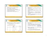
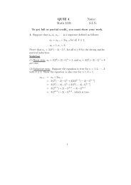
<strong>Chapter</strong> 3 <strong>Numerical</strong> <strong>Descriptive</strong> <strong>Measures</strong><br />
• <strong>Measures</strong> <strong>of</strong> central tendency<br />
Mean, median, mode, etc<br />
• <strong>Measures</strong> <strong>of</strong> variation<br />
Range, variance, standard deviation<br />
• <strong>Measures</strong> <strong>of</strong> position<br />
Quartile, percentile, standard score<br />
• Box-and-Whisker plot<br />
<br />
Five-number-summary<br />
• Mean<br />
<br />
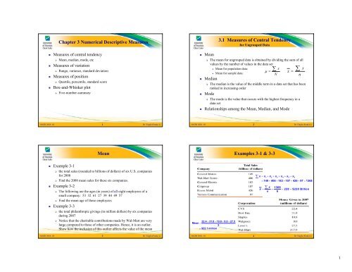
<strong>3.1</strong> <strong>Measures</strong> <strong>of</strong> <strong>Central</strong> Tendency<br />
for Ungrouped Data<br />
The mean for ungrouped data is obtained by dividing the sum <strong>of</strong> all<br />
values by the number <strong>of</strong> values in the data set<br />
• Mean for population data: x<br />
• Median<br />
• Mean for sample data:<br />
<br />
The median is the value <strong>of</strong> the middle term in a data set that has been<br />
ranked in increasing order<br />
• Mode<br />
The mode is the value that occurs with the highest frequency in a<br />
data set<br />
• Relationships among the Mean, Median, and Mode<br />
N<br />
x<br />
x <br />
n<br />
MATH 3038 - 01<br />
1<br />
Dr. Yingfu (Frank) Li<br />
MATH 3038 - 01<br />
2<br />
Dr. Yingfu (Frank) Li<br />
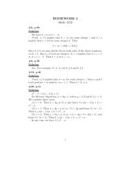
Mean<br />
Examples 3-1 & 3-3<br />
• Example 3-1<br />
the total sales (rounded to billions <strong>of</strong> dollars) <strong>of</strong> six U.S. companies<br />
for 2008<br />
Find the 2008 mean sales for these six companies.<br />
• Example 3-2<br />
The following are the ages (in years) <strong>of</strong> all eight employees <strong>of</strong> a<br />
small company: 53 32 61 27 39 44 49 57<br />
Find the mean age <strong>of</strong> these employees<br />
• Example 3-3<br />
the total philanthropic givings (in million dollars) by six companies<br />
during 2007<br />
Notice that the charitable contributions made by Wal-Mart are very<br />
large compared to those <strong>of</strong> other companies. Hence, it is an outlier.<br />
Show how the inclusion <strong>of</strong> this outlier affects the value <strong>of</strong> the mean<br />
22.4 31.8 19.8 9.0 27.5<br />
Mean <br />
5<br />
$22.1 million<br />
x x1 x2 x3 x4 x5 x6<br />
149 406 183 107 426 97 1368<br />
x 1368<br />
x 228 $228 Billion<br />
n 6<br />
MATH 3038 - 01<br />
3<br />
Dr. Yingfu (Frank) Li<br />
MATH 3038 - 01<br />
4<br />
Dr. Yingfu (Frank) Li<br />
1
MATH 3038 - 01<br />
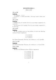
Median<br />
• How to find the median<br />
Rank the data set in increasing order.<br />
Find the middle term. The value <strong>of</strong> this term is the median.<br />
• Example <strong>of</strong> weight lost: 10, 5, 19, 8, 3<br />
Rank the data: 3, 5, 8, 10, 19<br />
Find the median: 3, 5, 8, 10, 19<br />
What if there are 6 numbers: 3, 5, 8, || 10, 13, 19<br />
• The median gives the center <strong>of</strong> a histogram, with half the<br />
data values to the left <strong>of</strong> the median and half to the right <strong>of</strong><br />
the median. The advantage <strong>of</strong> using the median as a measure<br />
<strong>of</strong> central tendency is that it is not influenced by outliers.<br />
Consequently, the median is preferred over the mean as a<br />
measure <strong>of</strong> central tendency for data sets that contain<br />
outliers.<br />
5<br />
Dr. Yingfu (Frank) Li<br />
MATH 3038 - 01<br />
Mode<br />
• The mode is the value that occurs with the highest frequency<br />
in a data set<br />
• Example 3-6<br />
The following data give the speeds (in miles per hour) <strong>of</strong> eight cars<br />
that were stopped on I-95 for speeding violations. 77 82 74 81 79 84<br />
74 78<br />
Find the mode.<br />
• A major shortcoming <strong>of</strong> the mode is that a data set may have<br />
none or may have more than one mode, whereas it will have<br />
only one mean and only one median.<br />
Unimodal: A data set with only one mode.<br />
Bimodal: A data set with two modes.<br />
Multimodal: A data set with more than two modes.<br />
6<br />
Dr. Yingfu (Frank) Li<br />
Relationships among Mean, Median, & Mode<br />
• For a symmetric histogram and frequency curve with one<br />
peak, the values <strong>of</strong> the mean, median, and mode are<br />
identical, and they lie at the center <strong>of</strong> the distribution.<br />
Relationships among Mean, Median, & Mode<br />
• For a histogram and a frequency curve skewed to the right,<br />
the value <strong>of</strong> the mean is the largest, that <strong>of</strong> the mode is the<br />
smallest, and the value <strong>of</strong> the median lies between these two.<br />
(Notice that the mode always occurs at the peak point.) The<br />
value <strong>of</strong> the mean is the largest in this case because it is<br />
sensitive to outliers that occur in the right tail. These outliers<br />
pull the mean to the right.<br />
MATH 3038 - 01<br />
7<br />
Dr. Yingfu (Frank) Li<br />
MATH 3038 - 01<br />
8<br />
Dr. Yingfu (Frank) Li<br />
2
Relationships among Mean, Median, & Mode<br />
• If a histogram and a distribution curve are skewed to the left,<br />
the value <strong>of</strong> the mean is the smallest and that <strong>of</strong> the mode is<br />
the largest, with the value <strong>of</strong> the median lying between these<br />
two. In this case, the outliers in the left tail pull the mean to<br />
the left.<br />
3.2 <strong>Measures</strong> <strong>of</strong> Dispersion<br />
for Ungrouped Data<br />
• Range = maximum value – minimum value<br />
• Variance<br />
Deviation from mean ( & )<br />
Kind <strong>of</strong> average <strong>of</strong> squared deviation<br />
<br />
Population variance<br />
<br />
Sample variance<br />
• Why divided by n-1, instead <strong>of</strong> by n for sample variance<br />
• Standard deviation = square root <strong>of</strong> variance<br />
Why do we need both variance and standard deviation<br />
• Population parameters and sample statistics<br />
MATH 3038 - 01<br />
9<br />
Dr. Yingfu (Frank) Li<br />
MATH 3038 - 01<br />
10<br />
Dr. Yingfu (Frank) Li<br />
Range<br />
Variance and Standard Deviation<br />
MATH 3038 - 01<br />
• Range = Largest value – Smallest Value<br />
• Example <strong>of</strong> two students’ test scores <strong>of</strong> a class<br />
A: 79 81 80; B: 80 100 60<br />
• Disadvantages<br />
The range, like the mean has the disadvantage <strong>of</strong> being influenced by<br />
outliers. Consequently, the range is not a good measure <strong>of</strong> dispersion<br />
to use for a data set that contains outliers.<br />
Its calculation is based on two values only: the largest and the<br />
smallest. All other values in a data set are ignored when calculating<br />
the range.<br />
11<br />
Dr. Yingfu (Frank) Li<br />
• The standard deviation is the most used measure <strong>of</strong> dispersion.<br />
• The value <strong>of</strong> the standard deviation tells how closely the values <strong>of</strong><br />
a data set are clustered around the mean.<br />
• In general, a lower value <strong>of</strong> the standard deviation for a data set<br />
indicates that the values <strong>of</strong> that data set are spread over a<br />
relatively smaller range around the mean.<br />
• In contrast, a large value <strong>of</strong> the standard deviation for a data set<br />
indicates that the values <strong>of</strong> that data set are spread over a<br />
relatively large range around the mean.<br />
• The Variance calculated for population data is denoted by σ² (read<br />
as sigma squared), and the variance calculated for sample data is<br />
denoted by s².<br />
• The standard deviation calculated for population data is denoted<br />
by σ, and the standard deviation calculated for sample data is<br />
denoted by s.<br />
MATH 3038 - 01<br />
12<br />
Dr. Yingfu (Frank) Li<br />
3
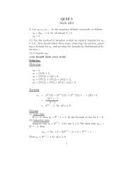
Calculation <strong>of</strong> Variance & Standard Deviation<br />
• Get deviations from the mean & then square the deviations<br />
• Kind <strong>of</strong> average <strong>of</strong> the squared deviations<br />
x (x - ) (x - ) 2<br />
80 80-75 = 5 5 2 = 25<br />
75 75-75 = 0 0 2 = 0<br />
75 75-75 = 0 0 2 = 0<br />
75 75-75 = 0 0 2 = 0<br />
70 70-75 = -5 (-5) 2 = 25<br />
Population Parameters and Sample Statistics<br />
• A numerical measure such as the mean, median, mode,<br />
range, variance, or standard deviation calculated for a<br />
population data set is called a population parameter, or<br />
simply a parameter.<br />
• A summary measure calculated for a sample data set is<br />
called a sample statistic, or simply a statistic.<br />
Slight difference in formula <strong>of</strong> population variance and sample<br />
variance<br />
MATH 3038 - 01<br />
13<br />
Dr. Yingfu (Frank) Li<br />
MATH 3038 - 01<br />
14<br />
Dr. Yingfu (Frank) Li<br />
3.3 Mean, Variance & Standard Deviation<br />
for Grouped Data<br />
• Grouped data in frequency table<br />
• Midpoint <strong>of</strong> each group (class) as approximate data point,<br />
and frequency as the number <strong>of</strong> such approximate points<br />
• Then follow the conventional definitions for mean, variance,<br />
and standard deviation<br />
• Mean for Grouped Data<br />
mf<br />
Mean for population data <br />
N mf<br />
Mean for sample data<br />
x <br />
n<br />
• Variance and Standard Deviation for Grouped Data<br />
Mean for Grouped Data<br />
• Table 3.8 gives the frequency distribution <strong>of</strong> the daily<br />
commuting times (in minutes) from home to work for all 25<br />
employees <strong>of</strong> a company.<br />
• Calculate the mean <strong>of</strong> the daily commuting times.<br />
Equivalent to data set: 5, 5, 5, 5; 15, 15, 15, 15, 15, 15, 15,<br />
15, 15; 25, 25, 25, 25, 25, 25; 35, 35, 35, 35; 45, 45 Mean = 535 / 25 = 21.4<br />
MATH 3038 - 01<br />
15<br />
Dr. Yingfu (Frank) Li<br />
MATH 3038 - 01<br />
16<br />
Dr. Yingfu (Frank) Li<br />
4
Variance for Grouped Data<br />
Examples <strong>of</strong> Variance for Grouped Data<br />
• Same data as the previous slide<br />
• Example 3-16: Table 3.8 gives the frequency distribution <strong>of</strong><br />
the daily commuting times (in minutes) from home to work<br />
for all 25 employees <strong>of</strong> a company. Calculate the variance<br />
and standard deviation.<br />
• Example 3-17: Table <strong>3.1</strong>0 gives the frequency distribution <strong>of</strong><br />
the number <strong>of</strong> orders received each day during the past 50<br />
days at the <strong>of</strong>fice <strong>of</strong> a mail-order company. Calculate the<br />
variance and standard deviation.<br />
MATH 3038 - 01<br />
17<br />
Dr. Yingfu (Frank) Li<br />
MATH 3038 - 01<br />
18<br />
Dr. Yingfu (Frank) Li<br />
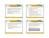
3.4 Use <strong>of</strong> Standard Deviation<br />
Chebyshev’s Theorem<br />
• Chebyshev’s Theorem<br />
For any number k greater than 1, at least (1 – 1/k²) <strong>of</strong> the data values<br />
lie within k standard deviations <strong>of</strong> the mean.<br />
• Empirical Rule<br />
<br />
For a bell shaped distribution approximately<br />
• 68% <strong>of</strong> the observations lie within one standard deviation <strong>of</strong> the mean<br />
• 95% <strong>of</strong> the observations lie within two standard deviations <strong>of</strong> the mean<br />
• 99.7% <strong>of</strong> the observations lie within three standard deviations <strong>of</strong> the<br />
mean<br />
k = 2 (3), area ≥ 75% (89%)<br />
MATH 3038 - 01<br />
19<br />
Dr. Yingfu (Frank) Li<br />
MATH 3038 - 01<br />
20<br />
Dr. Yingfu (Frank) Li<br />
5
Example 3-18<br />
Illustration <strong>of</strong> the Empirical Rule<br />
• The average systolic blood pressure for 4000 women who<br />
were screened for high blood pressure was found to be 187<br />
with a standard deviation <strong>of</strong> 22. Using Chebyshev’s theorem,<br />
find at least what percentage <strong>of</strong> women in this group have a<br />
systolic blood pressure between 143 and 231.<br />
• μ = 187 and σ = 22<br />
143 μ = 187<br />
231<br />
• k = 44/22 = 2<br />
• The percentage is at least<br />
1 1 1<br />
1 1<br />
1<br />
1.25<br />
k<br />
2<br />
(2) 4<br />
2<br />
<br />
.75<br />
or 75%<br />
MATH 3038 - 01<br />
21<br />
Dr. Yingfu (Frank) Li<br />
MATH 3038 - 01<br />
22<br />
Dr. Yingfu (Frank) Li<br />
Example 3-19<br />
Example 3-19<br />
• The age distribution <strong>of</strong> a sample <strong>of</strong> 5000 persons is bellshaped<br />
with a mean <strong>of</strong> 40 years and a standard deviation <strong>of</strong><br />
12 years. Determine the approximate percentage <strong>of</strong> people<br />
who are 16 to 64 years old.<br />
1. Compare the<br />
numbers with<br />
the mean<br />
2. Check how<br />
many standard<br />
deviations the<br />
number is away<br />
from the mean<br />
• The age distribution <strong>of</strong> a sample <strong>of</strong> 5000 persons is bellshaped<br />
with a mean <strong>of</strong> 40 years and a standard deviation <strong>of</strong><br />
12 years.<br />
Determine the approximate percentage <strong>of</strong> people who are 28 to 64<br />
years old.<br />
Determine the approximate percentage <strong>of</strong> people who are 16 to 52<br />
years old.<br />
Determine the approximate percentage <strong>of</strong> people who are 52 years<br />
or old.<br />
Determine the approximate percentage <strong>of</strong> people who are 28 years<br />
or young.<br />
MATH 3038 - 01<br />
23<br />
Dr. Yingfu (Frank) Li<br />
MATH 3038 - 01<br />
24<br />
Dr. Yingfu (Frank) Li<br />
6
3.5 <strong>Measures</strong> <strong>of</strong> Position<br />
Quartiles and Percentiles<br />
• Quartiles: Q1, Q2, Q3<br />
Divide the ranked data into four equal parts<br />
Interquartile range = Q3 – Q1<br />
Box-and-Whisker Plot<br />
• Percentile: P1, P2, …, P99<br />
Divide the ranked data into 100 equal parts<br />
Q1 = P25, Q2 = P50 = median, Q3 = P75<br />
• Standard score<br />
Use for comparison <strong>of</strong> different subjects<br />
MATH 3038 - 01<br />
25<br />
Dr. Yingfu (Frank) Li<br />
MATH 3038 - 01<br />
26<br />
Dr. Yingfu (Frank) Li<br />
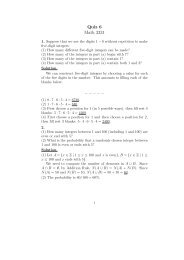
Examples 3-20 & 3-21<br />
Percentiles and Percentile Rank<br />
• Example 3-20, which gives the 2008 pr<strong>of</strong>its (rounded to<br />
billions <strong>of</strong> dollars) <strong>of</strong> 12 companies selected from all over<br />
the world – see the book<br />
Find the values <strong>of</strong> the three quartiles. Where does the 2008 pr<strong>of</strong>its <strong>of</strong><br />
Merck & Co fall in relation to these quartiles<br />
Find the interquartile range.<br />
• Example 3-21. The following are the ages (in years) <strong>of</strong> nine<br />
employees <strong>of</strong> an insurance company:<br />
47 28 39 51 33 37 59 24 33<br />
Find the values <strong>of</strong> the three quartiles. Where does the age <strong>of</strong> 28 fall<br />
in relation to the ages <strong>of</strong> the employees<br />
Find the interquartile range.<br />
• Calculating Percentiles<br />
The (approximate) value <strong>of</strong> the k th percentile, denoted by P k , is<br />
kn <br />
P k<br />
Value <strong>of</strong> the th term in a ranked data set<br />
100<br />
<br />
where k denotes the number <strong>of</strong> the percentile and n represents the<br />
sample size<br />
Example 3-22<br />
• Finding Percentile Rank <strong>of</strong> a Value<br />
Number <strong>of</strong> valuesless than xi<br />
Percentilerank <strong>of</strong> xi<br />
<br />
100<br />
Totalnumber <strong>of</strong> valuesin thedata set<br />
Examples 3-22 & 3-23<br />
• Different packages might give you different answers<br />
Excel<br />
Minitab<br />
MATH 3038 - 01<br />
27<br />
Dr. Yingfu (Frank) Li<br />
MATH 3038 - 01<br />
28<br />
Dr. Yingfu (Frank) Li<br />
7
3.6 Box-and-Whisker Plot<br />
• Five-Number Summary<br />
Min, Q1, Q2=Median, Q3, Max<br />
• A plot that shows the center, spread, and skewness <strong>of</strong> a data<br />
set. It is constructed by drawing a box and two whiskers that<br />
use the median, the first quartile, the third quartile, and the<br />
smallest and the largest values in the data set between the<br />
lower and the upper inner fences.<br />
• Formal BW plot<br />
Also used to detect potential outliers<br />
Box = Q1, Q2, Q3<br />
Whisker<br />
• Inner fences: 1.5 times <strong>of</strong> IQR away from Q1(Q3)<br />
• Outer fences: 3 times <strong>of</strong> IQR away from Q1(Q3)<br />
Example 3-24<br />
• The following data are the incomes (in thousands <strong>of</strong> dollars)<br />
for a sample <strong>of</strong> 12 households.<br />
75 69 84 112 74 104 81 90 94 144 79 98<br />
Construct a box-and-whisker plot for these data.<br />
Step 1: calculate Q1, Q2, Q3 & IQR<br />
Step 2: calculate 1.5 x IQR and find the lower (upper) inner fence =<br />
Q1 – (+) 1.5 x IQR<br />
Step 3: locate the smallest (largest) values within the two inner<br />
fences<br />
Step 4: draw box and whiskers<br />
Step 5: uses and misuses<br />
• Detecting outliers is a challenging problem<br />
MATH 3038 - 01<br />
29<br />
Dr. Yingfu (Frank) Li<br />
MATH 3038 - 01<br />
30<br />
Dr. Yingfu (Frank) Li<br />
Standard Score<br />
Technology Instruction<br />
• Standard score defined as<br />
Use for comparison<br />
• An example: compare Mike’s height (78 ins) with Rebecca’s<br />
height (76 ins)<br />
NBA players: average height = 69 ins & s = 2.8 ins<br />
<br />
<br />
• Mike Jordan’s std height is<br />
WNBA players: average height = 63.6 ins & s = 2.5 ins<br />
• Rebecca Lobo’s std height is<br />
Who has advantage in height when they play<br />
• TI – 84 / 83 plus<br />
• Minitab<br />
• Excel<br />
MATH 3038 - 01<br />
31<br />
Dr. Yingfu (Frank) Li<br />
MATH 3038 - 01<br />
32<br />
Dr. Yingfu (Frank) Li<br />
8