Generalized-gradient-approximation noninteracting free-energy ...

KARASIEV, SJOSTROM, AND TRICKEY PHYSICAL REVIEW B 86, 115101 (2012)
ν(t)
2.5
2
1.5
1
0.5
0
0.01 0.1 1 10
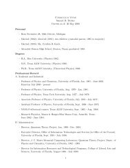
FIG. 12. ν(t) as defined by Eq. (B2).
satisfactory results. In the T → 0 limit, all ftGGA free energy
functionals should reduce to known zero-temperature kinetic
energy functionals, a fact we have used to present a rather
simple ftGGA.
Numerical implementation of the OF-DFT calculations in
a plane-wave basis requires a local pseudopotential which we
have presented. Comparison of finite temperature OF-DFT
and KS calculations on sc-H over a wide range of material
densities for electronic temperatures up to 100 000 K leads to
the conclusions that two ftGGA functionals, namely KST2
and VWTF, provide the overall best results and that the
relative error in the high density regime is small for all
functionals.
ACKNOWLEDGMENTS
We acknowledge informative conversations with Frank
Harris and Jim Dufty with thanks. This work was supported
in substantial part by the US Dept. of Energy TMS Grant No.
DE-SC0002139.
APPENDIX A
The temperature scaling function κ introduced in Eq. (16)
may be written by use of Eqs. (9) and (15) as
t
) −5/3
κ(βμ) = 5 ( 3
2 2 I 1/2(βμ)
[
× − 2 ]
3 I 3/2(βμ) + βμI 1/2 (βμ) . (A1)
By use of Eq. (14), we may eliminate (βμ) infavoroft
in Eq. (A1). We have done that numerically. With that result,
we can present κ(t) analytically as an adapted form of Perrot’s
free energy fit. 16 See below. The functions ζ (t) and ξ(t) may
be calculated using relations with κ(t) giveninEqs.(18)
and (19). In addition, we provide an adapted analytical ˜h(t).
Both functions are split into regions t t 0 and t t 0 , where
t 0 = 4(2/3π 2 ) 1/3 /3, to take account of the different asymptotic
forms of the Fermi integrals for (βμ) ≪ 0 and (βμ) ≫ 0.
For t t 0 = 0.543010717965,
κ(t) =−2.5t ln(t) − 2.141088549t + 0.2210798602t −0.5
+ 0.7916274395 × 10 −3 t −2 − 0.4351943569
× 10 −2 t −3.5 + 0.4188256879 × 10 −2 t −5
− 0.2144912720 × 10 −2 t −6.5 + 0.5590314373
× 10 −3 t −8 − 0.5824689694 × 10 −4 t −9.5 (A2)
˜h(t) = 3 − 0.7996705242t −1.5 + 0.2604164189t −3
− 0.1108908431t −4.5 + 0.6875811936 × 10 −1 t −6
− 0.3515486636 × 10 −1 t −7.5 + 0.1002514804
× 10 −1 t −9 − 0.1153263119 × 10 −2 t −10.5 . (A3)
For t t 0 = 0.543010717965,
κ(t) = 1 − 4.112335167t 2 + 1.995732255t 4 + 14.83844536t 6
− 178.4789624t 8 + 992.5850212t 10 − 3126.965212t 12
+ 5296.225924t 14 − 3742.224547t 16 (A4)
˜h(t) = 1 + 3.210141829t 2 + 58.30028308t 4 − 887.5691412t 6
+ 6055.757436t 8 − 22429.59828t 10 + 43277.02562t 12
− 34029.06962t 14 .
APPENDIX B
(A5)
We outline a route to simplified GGAs which is a potential
alternative to the one given in the discussion of Eqs. (37)–(39).
Equations (37) obviously combine to give
Fσ SGA (s σ ) = 2 + 5 (
s
2
27 τ − sσ 2 )
− F
SGA
τ (s τ ). (B1)
As suggested in the discussion in conjunction with Fig. 2, the
ratio
ν(t) := [s σ (t)/s τ (t)] 2
(B2)
is a smooth, bounded [0 ν(t) 2.2] function. See Fig. 12.
With this function, Eq. (B1) becomes
F SGA
σ (s σ ) = 2 + 5
27 s2 τ
[1 − ν(t)] − F
SGA
τ (s τ ). (B3)
Utilization to form a GGA is via
Fσ GGA (s σ ) = 2 + 5
27 s2 τ [1 − νGGA (t)] − Fτ GGA (s τ ), (B4)
where the superscript “GGA” on ν indicates use of some
judiciously selected approximate representation of ν(t). This
choice can be constrained by insertion of the form from
Eq. (B4) in Eq. (35). We have this approach under study.
* vkarasev@qtp.ufl.edu
1 N. D. Mermin, Phys. Rev. 137, A1441 (1965).
2 M. V. Stoitsov and I. Zh. Petkov, Ann. Phys. 184, 121 (1988).
3 R. M. Dreizler, in The Nuclear Equation of State, Part A, edited
by W. Greiner and H. Stöcker, NATO ASI Vol. B216 (Plenum,
NY, 1989), p. 521.
115101-10