Generalized-gradient-approximation noninteracting free-energy ...

PHYSICAL REVIEW B 86, 115101 (2012)
Generalized-gradient-approximation noninteracting free-energy functionals for orbital-free density
functional calculations
Valentin V. Karasiev, * Travis Sjostrom, and S. B. Trickey
Quantum Theory Project, Departments of Physics and of Chemistry, P.O. Box 118435, University of Florida, Gainesville,
Florida 32611-8435, USA
(Received 20 June 2012; published 4 September 2012)
We develop a framework for orbital-free generalized gradient approximations (GGAs) for the noninteracting
free energy density and its components (kinetic energy, entropy) based upon analysis of the corresponding gradient
expansion. From that we obtain a new finite-temperature GGA (ftGGA) pair. We discuss implementation of the
finite-temperature Thomas-Fermi, second-order gradient expansion, and our new ftGGA free energy functionals
in an orbital-free density functional theory (OF-DFT) code, including the construction and validation of required
local pseudopotentials. Then we compare results of self-consistent OF-DFT calculations on hydrogen using those
noninteracting free energy functionals (in combination with the zero-temperature local density approximation
(LDA) for exchange-correlation) with results from conventional finite-temperature Kohn-Sham calculations and
the same LDA. As an aid to implementation, we provide analytical expressions for the temperature-dependent
scaling factors involved.
DOI: 10.1103/PhysRevB.86.115101
PACS number(s): 31.15.E−,71.15.Mb, 05.70.Ce, 65.40.G−
I. INTRODUCTION
Warm dense matter (WDM) is characterized by elevated
temperature (up to one hundred eV) and high pressures
(up to hundreds of TPa). These characteristics differ greatly
from those in standard condensed matter physics, yet such
temperatures and pressures are not high enough to make
standard plasma physics methods fully applicable. The typical
present-day theoretical and computational approach to
WDM thus is a combination of finite-temperature density
functional theory to describe the electrons 1–3 and classical
molecular dynamics for ions. Finite-temperature DFT for the
electronic degrees of freedom is realized via the Kohn-Sham
(KS) procedure. It becomes computationally very expensive
at elevated temperature because of the large number of
fractionally occupied KS orbitals which must be taken into
account. (The computational cost of solving the KS equations
in an atom-centered basis scales in principle as N 4 , where
N is proportional to the number of occupied KS orbitals.
Obviously N increases with temperature. Variational Coulomb
fitting 4 reduces the scaling to N 3 . In a plane-wave basis with
pseudopotentials, the general scaling is N 3 also. Less costly
schemes eventually exploit some form of matrix sparsity, thus
are not generally applicable.)
In contrast, the orbital-free version of density functional
theory (OF-DFT) is, in principle at least, a much less
expensive alternative to the orbital-based KS method for both
zero-temperature and finite-temperature calculations. OF-DFT
scales only with the cell size, so the computational cost of a
well-implemented OF-DFT scheme should be about the same
for both zero- and finite-temperature regimes.
OF-DFT at zero temperature requires reliable approximations
for the exchange-correlation (XC) and noninteracting
kinetic energy (KE) T s density functionals. These two contribute
to the total energy E tot with substantially different
magnitudes: T s ≈|E tot | while |E xc | is about one order of
magnitude smaller. Because of this disparity, development of
accurate approximate OF-KE functionals is a challenging task
which has not reached the refinement of E xc functionals.
The standard developmental approach to nonempirical E xc
approximations invokes a sequence of added functional variables,
hence the local density approximation (LDA), gradient
expansion approximation (GEA) and generalized gradient approximations
(GGA), meta-GGAs (which add the KE density
or Laplacian of the density), etc. Functional construction is
facilitated by enforcement of known properties of the exact
5
functional. Examples include the highly popular PBE E x,GGA
and proposed improvements on it. 6–8 The GGA approach to
the KE functional also is based on satisfaction of some of
the known exact conditions on this functional. 9,10 “Modified
conjoint” GGA type KE functionals, 11,12 for example, are
constrained to satisfy one of the important exact conditions,
namely, positivity of the functional itself and of the so-called
Pauli potential associated with it.
Fortunately, the high density and elevated temperature
of the WDM regime are favorable for use of the OF-DFT
approach. In finite-temperature OF-DFT, the task is to approximate
the entire free energy (including the noninteracting KE,
noninteracting entropy, and XC) as a functional of the electronic
density. At present, the basic Thomas-Fermi (TF) 13,14
model and TF with gradient corrections are the dominant
computational approaches in finite-temperature OF-DFT. 15,16
Renewed interest in better free-energy density functionals is
exemplified by two recent studies of their scaling behavior. 17,18
Here we develop a finite-temperature GGA (ftGGA) approximation
for the noninteracting free energy functional. ftGGA
is a nontrivial extension of the zero-temperature GGA to finite
temperatures for, as we shall show, it should depend upon
explicitly temperature-dependent variables which are defined
on the basis of the gradient expansion for the kinetic and
entropic contributions to the free energy. Those variables
play roles analogous with the reduced density gradient in
ground-state functionals.
Pseudopotentials (PPs) are an important implementational
challenge in this context. Standard Kohn-Sham calculations
on extended, periodically bounded systems most commonly
employ PP techniques. In DFT codes of both the plane-wave
1098-0121/2012/86(11)/115101(11) 115101-1
©2012 American Physical Society

KARASIEV, SJOSTROM, AND TRICKEY PHYSICAL REVIEW B 86, 115101 (2012)
and numerical grid varieties, PPs reduce computational cost by
eliminating the bare Coulomb nuclear-electron singularity and
by reducing (substantially) the number of active electrons in
the self-consistent field (SCF) procedure. The most common
standard PPs are nonlocal (see for example Refs. 19–21), i.e.,
there is a different operator for each atomic orbital angular
momentum. While the computational cost of OF-DFT does
not depend on the total number of electrons, the problems
from the singularity of the bare Coulomb external potential
remain if one intends to use a plane-wave basis or numerical
grid. For OF-DFT in such an implementation, a local PP or
regularized potential is inescapable.
II. ORBITAL-FREE NON-INTERACTING FREE ENERGY
FUNCTIONALS
A. Finite-temperature DFT summary
For development of the finite-temperature version of DFT
it is customary to work in the grand canonical ensemble. The
grand canonical potential of a system of electrons in an external
potential v(r) with electronic density n(r), chemical potential
μ, and temperature T can be written as a functional of the
density 1,2 ∫
[n] = F[n] + (v(r) − μ)n(r)dr. (1)
The universal free-energy functional F[n] has the decomposition
F[n] = F s [n] + F H [n] + F xc [n], (2)
where F s [n] is the noninteracting free energy, F H [n] is
the classical Coulomb repulsion energy, and F xc [n] isthe
exchange-correlation contribution to the free energy. In order,
these are
F s [n] = T s [n] − T S s [n], (3)
where T s and S s are the noninteracting kinetic energy and
entropy respectively, and
F H [n] = 1 2
∫∫ n(r)n(r ′ )
|r − r ′ | drdr′ (4)
is the Hartree (classical Coulomb repulsion) energy. The
exchange-correlation (XC) functional is
F xc [n] = (T [n] − T s [n]) − T (S[n] − S s [n])
+ (U ee [n] − F H [n]). (5)
In it, T [n] and S[n] are the fully interacting system kinetic
energy and entropy, respectively, and U ee is the full electronelectron
Coulomb interaction energy.
B. Thomas-Fermi approximation
Evaluation of the grand potential Eq. (1) for the noninteracting
uniform electron gas (UEG) of constant density n in a
volume V (with uniform background for charge neutrality; see
discussion on this point in Ref. 22) gives the UEG free energy,
( ∂
Fs
UEG (n,T ) = UEG
UEG
)
s (n)
s (n) − μ
∂μ T,V
√ [ 2
= V − 2 ]
π 2 β 5/2 3 I 3/2(βμ) + βμI 1/2 (βμ) . (6)
Here, β = (k B T ) −1 and I α is the Fermi-Dirac integral 23
∫ ∞
I α (η) := dx
0 1 + exp(x − η) , α > −1 (7)
I α−1 (η) = 1 d
α dη I α(η).
The chemical potential μ is determined from
n =− 1 √
∂
2
V ∂μ∣ =
T,V π 2 β I 1/2(βμ). (8)
3/2
Invocation of the local density approximation gives the
Thomas-Fermi (TF) 13,14 noninteracting free energy density 15
as
( )∣ 1 ∣∣∣n=n(r)
fs
TF (n(r),T ) ≡
V F s
UEG
√ [ 2
= − 2 ]
π 2 β 5/2 3 I 3/2(βμ) + βμI 1/2 (βμ) . (9)
Here μ is the local TF chemical potential defined by n(r)
through Eq. (8), and not the chemical potential of the
nonuniform system. The LDA noninteracting free energy
functional is then
∫
F TF
s [n] =
x α
f TF
s (n(r),T )dr. (10)
The corresponding entropy and kinetic energy densities then
follow from Eq. (9):
σs
TF
TF
∂fs (n,T )
(n,T ) =− ∂T ∣
n
√ [ 2 5
=
π 2 β 5/2 T 3 I 3/2(βμ) − βμI 1/2 (βμ)]
, (11)
and
τ TF
s
(n,T ) = fs
TF (n,T ) + Tσs TF (n,T )
=
In terms of the reduced temperature
Eq. (8) gives
t = T/T F =
√
2
π 2 β 5/2 I 3/2(βμ). (12)
2
, (13)
β[3π 2 n(r)]
2/3
I 1/2 (βμ) = nπ 2 β 3/2
√ = 2 . (14)
2 3t
3/2
Because I 1/2 (x) is strictly increasing with x,(βμ) is a function
of t, hence all functions of (βμ) are functions of t. Asa
consequence, the entire term in brackets in Eq. (9) also is
115101-2

GENERALIZED-GRADIENT-APPROXIMATION ... PHYSICAL REVIEW B 86, 115101 (2012)
a function of t. This insight, in combination with the zerotemperature
TF kinetic energy density,
τ0 TF (n) = 3
10 (3π 2 ) 2/3 n 5/3 = 2 √
2
, (15)
5 π 2 β 5/2 t
5/2
allows Eq. (9) to be presented in the factorized form
where
f TF
s
(n,T ) = τ TF (n)κ(t) (16)
0
κ(t) := 5 [
2 t 5/2 − 2 ]
3 I 3/2(βμ) + βμI 1/2 (βμ) . (17)
To facilitate computation, an analytical fit to κ(t) is provided
in Appendix A.
The correspondingly factorized entropy and kinetic energy
densities may be found from Eq. (16) as
σs
TF
TF
∂fs (n,T )
(n,T ) =− ∂T ∣ ≡ 1
n T τ 0 TF (n)ζ (t), (18)
ζ (t) =−t ∂κ(t)
∂t
and
τ TF
s
(n,T ) = f TF
s
(n,T ) + Tσ TF
ξ(t) = κ(t) − t ∂κ(t) .
∂t
s
(n,T ) ≡ τ TF
0 (n)ξ(t) (19)
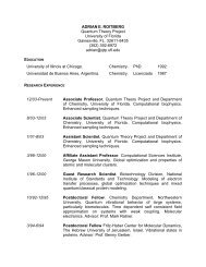
Figure 1 shows the functions κ(t), ζ (t), ξ(t), and ˜h(t). (The
last-named of these is discussed in the next section.)
The zero-temperature limit for the entropic contribution
Tσs
TF and the kinetic energy τs TF may be found from Eqs. (11)
and (12):
lim
T →0 TσTF s (n,T ) = 0, (20)
and
lim τ s
TF
T →0
= τ0 TF (n). (21)
To evaluate these limits, the properties of Fermi-Dirac
integrals, lim β→∞ I 1/2 (βμ) = 2 3 (βμ)3/2 , lim β→∞ I 3/2 (βμ) =
2
5 (βμ)5/2 , and the relation n = (2μ) 3/2 /(3π 2 ) obtained from
4
3
2
1
0
-1
κ
ξ
ζ
72h
-2
0.01 0.1 1 10
t
FIG. 1. Behavior of functions κ, ζ , ξ,and ˜h ≡ 72h.
Eq. (8) in the limit β →∞ were used. From Eqs. (20)
and (21) [alternatively, from Eqs. (18) and (19)] and from
the non-negativity of the entropy, Eq. (11), and the kinetic
energy density, it follows that
and
lim
T →0 ζ (t) = 0, (22)
ζ (t) 0,∀t,
lim
T →0 ξ(t) = 1, (23)
ξ(t) 0,∀ t.
C. Gradient expansion
The zero-temperature gradient correction to the Thomas-
Fermi model was generalized to finite temperatures by
Perrot, 16 with higher order corrections given in Ref. 23. In
the limit T → 0, that generalization reduces to the zerotemperature
second-order gradient approximation (SGA). 24
The finite-temperature gradient term has the form of the
von Weizsäcker 25 (VW) kinetic energy density, t W (n,∇n) =
|∇n| 2 /(8n), scaled by a function h(t) of the reduced temperature,
namely
fs
SGA (n,∇n,T ) = fs TF (n,T ) + 8h(t)t W (n,∇n). (24)
This follows by elimination of βμin favor of t [recall Eq. (14)]
in Perrot’s expression 16
h(t) =− 1 I 1/2 (βμ)I −3/2 (βμ)
24 I−1/2 2 (βμ) . (25)
It is convenient to use the quantity ˜h(t) = 72h(t), because
lim t→0 ˜h(t) = 1, which allows us to write the full von
Weizsäcker term as ˜ht W and the corresponding SGA in the
more familiar form (1/9) ˜ht W . We adopt the analytical fit of
Eq. (25) given in Ref. 16 to a function of reduced temperature
t as shown in Appendix A.
For further analysis, it is convenient to introduce the
reduced density gradient familiar in zero-temperature GGAs
for exchange and KE, namely
s(n,∇n) ≡
|∇n|
(2k F )n = 1 |∇n|
, (26)
2(3π 2 ) 1/3 n4/3 and rewrite Eq. (24) as
f SGA
s
(n,∇n,T ) = τ TF
0
(n)κ(t) + τ
TF
0 (n) 5 27 s2 ˜h(t), (27)
where the VW term is rewritten as t W = 5 3 τ 0 TFs2
.
The kinetic energy and entropy contributions to the free
energy functional defined by Eq. (27) may be evaluated as
usual (see also Refs. 23 and 26). First,
σs
SGA
SGA
∂fs (n,∇n,T )
(n,∇n,T ) =−
∂T
∣
∣
n
= 1 T τ TF
0 (n)ζ (t) (
1 − 5
27 s2 t
ζ (t)
)
d ˜h(t)
.
dt
(28)
115101-3

KARASIEV, SJOSTROM, AND TRICKEY PHYSICAL REVIEW B 86, 115101 (2012)
Then τ SGA
s
= f SGA
s
+ Tσ SGA
s
gives
τs SGA (n,∇n,T )
(
= τ0 TF (n)ξ(t) 1 + 5 1
27 s2 ξ(t)
[
˜h(t) − t d ])
˜h(t)
, (29)
dt
where we have taken into account the definition Eq. (13) and
simplified the derivative term in Eqs. (28) and (29) according
to T [∂ ˜h(t)/∂T ] n = td ˜h(t)/dt. In the zero-temperature limit,
the entropic contribution to the free energy of course vanishes,
lim T →0 (Tσs
SGA ) = 0, and the kinetic energy part reduces to
the zero-temperature SGA kinetic energy, lim T →0 τs SGA =
τ0 TF(n)(1
+ 5 3 s2 ).
D. Finite-temperature generalized gradient approximation
The underlying concept of GGAs in zero-temperature XC
and KE functionals is to take into account the physical
content of higher-order terms in the gradient expansion and
effects beyond the slowly varying density approximation while
avoiding difficulties associated with use of a strict secondorder
expansion as a general functional. For X and KE, this
generalization is done by multiplying the relevant LDA (zeroorder
term) energy density by an enhancement factor which
is a functional of the reduced density gradient s, Eq.(26).
Both the analytical form and parameters of the enhancement
factors may be defined (or at least constrained) by imposition
of known exact conditions. We follow an analogous strategy
here for the finite-temperature noninteracting system.
The correction terms in Eqs. (27)–(29) are the first terms
of a general gradient expansion for the noninteracting free
energy and its components (again, see Refs. 23 and 26). In the
finite-temperature case, the structure of Eqs. (28) and (29)
suggests that we define corresponding finite-temperature
reduced density gradients as
√
td ˜h(t)/dt
s σ (n,∇n,T ) = s(n,∇n) ,
ζ (t)
√ (30)
˜h(t) − td ˜h(t)/dt
s τ (n,∇n,T ) = s(n,∇n)
,
ξ(t)
for use in the entropy and kinetic energy, respectively. It is
straightforward to show that in the zero-temperature limit
lim s τ (n,∇n,T ) = s(n,∇n). (31)
T →0
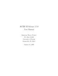
Figure 2 shows the ratios (s τ /s) 2 and (s σ /s) 2 as functions
of reduced temperature t. Both are smooth, non-negative
functions with some structure at intermediate t. Both vanish at
t ≫ 1. The ratio (s τ /s) 2 goes to a constant at t ≪ 1, namely
lim t→0 (s τ /s) 2 = 1. Direct numerical evaluation shows that
(s σ /s) 2 ≈ 0.8 fort ≪ 1.
With this information, we may define the finite-temperature
GGA free energy functional form as
∫
Fs ftGGA [n,T ] = τ0 TF (n)ξ(t)F τ (s τ )dr
∫
− τ0 TF (n)ζ (t)F σ (s σ )dr, (32)
1.5
1
0.5
(s τ
/s) 2
(s σ
/s) 2
0
0.001 0.01 0.1 1 10 100
t
FIG. 2. Functions (s τ /s) 2 and (s σ /s) 2 .
where F τ and F σ are the noninteracting kinetic energy
and entropic enhancement factors depending on reduced
density gradients s τ and s σ correspondingly. The definitions
in Eq. (32) are generalizations of the second-order
gradient expansion of the noninteracting free energy components
in Eqs. (28) and (29) in the form of zeroth-order
terms multiplied by corresponding enhancement factors.
Notice that this definition automatically ensures that the
entropic and KE contributions scale correctly, since T S s
and T s scale identically. 17,18 Specifically, Ts ftGGA [n λ ,T ] =
λ 2 Ts
ftGGA [n,T /λ 2 ] and Ss
ftGGA [n λ ,T ] = Ss
ftGGA [n,T /λ 2 ], with
n λ (r) = λ 3 n(λr). All of the scaling is in τ0 TF (n). All the
other factors in the integrands in Eq. (32) are dimensionless
functions of dimensionless variables.
The two RHS terms in Eq. (32) should be interpretable as the
kinetic energy (Ts
ftGGA ) and entropic (T Ss
ftGGA ) contributions.
To enforce this interpretation, we invoke the thermodynamic
relation
S ftGGA
s
=−
=−
∂F
ftGGA
s
∂T
∂T
ftGGA
s
∂T
∣
∣
N,V
∣ + ∂( )
T Ss
ftGGA
N,V ∂T ∣ , (33)
N,V
which can be rearranged as
∂Ts
ftGGA
∂T ∣ = T ∂SftGGA
s
N,V ∂T ∣ . (34)
N,V
Interchange of integration and partial derivative evaluation
gives a relation between F τ and F σ ,
ξ ′ (t)F τ (s τ ) + ξ(t)F τ ′ (s τ ) ∂s τ
∂t
=− 1 t ζ (t)F σ (s σ ) + ζ ′ (t)F σ (s σ ) + ζ (t)F σ ′ (s σ ) ∂s σ
∂t . (35)
Primes denote derivatives with respect to corresponding
arguments, i.e., with respect to t, s τ ,ors σ . Whether or not
Eq. (35) is satisfied exactly by a pair of proposed F τ and F σ
enhancement factors, Eq. (33) always can be used to obtain the
entropic contribution, T Ss
ftGGA , corresponding to a specified
115101-4

GENERALIZED-GRADIENT-APPROXIMATION ... PHYSICAL REVIEW B 86, 115101 (2012)
ftGGA functional Eq. (32):
T Ss
ftGGA
ftGGA
∂Fs [n,T ]
[n,T ] =−T ∂T ∣
N,V
∫ [
= τ0 TF (n)t − ξ ′ (t)F τ (s τ ) − ξ(t)F τ ′ (s τ ) ∂s τ
+ ζ ′ (t)F σ (s σ ) + ζ (t)F ′ σ (s σ ) ∂s σ
∂t
∂t
]
dr. (36)
There is motivation to satisfy Eq. (35) since the scaling factors
ξ and ζ already constrain the terms of Eq. (32) to be the kinetic
and entropic pieces, respectively, in both the zero-temperature
and Thomas-Fermi limits.
However, use of Eq. (35) to determine one of the enhancement
factors when the other is given is not straightforward in
general. The SGA functionals Eqs. (28) and (29), which do
satisfy Eq. (35), provide a clue to a simpler approximate route.
Those functionals can be written in the form of Eq. (32) with
enhancement factors
Fτ SGA (s τ ) = ( )
1 + 5
27 s2 τ
(37)
Fσ SGA (s σ ) = ( )
1 − 5
27 s2 σ .
Thus, the two SGA enhancement factors are related by
Fσ
SGA (s σ ) = 2 − Fτ SGA (s σ ). (38)
Equation (38) can be generalized in the usual spirit of GGAs
by requiring that the entropic contribution enhancement factor
associated with a chosen F τ (s τ ), Eq. (32),is
F σ (s σ ) ≈ 2 − F τ (s σ ). (39)
In general, a pair of enhancement factors related in this way
will not satisfy Eq. (35) precisely. The main consequence
of such a failure is that the two terms in Eq. (32) may not
be interpretable strictly as kinetic and entropic contributions.
Instead, Eq. (36) gives the entropic contribution, Eq. (32) gives
the noninteracting free energy, and the kinetic energy functional
is T s [n,T ] = F s [n,T ] + T S s [n,T ]. A complementary
discussion to this approach is given in Appendix B.
The requirement that the zero-temperature limit of the
functional Fs
ftGGA [n,T ], Eq. (32), should reduce to the zerotemperature
GGA kinetic energy, in conjunction with the
factorized form of the integrand, leads to the realization that
the simplest approximation for a finite-temperature GGA F τ
is to use a zero-temperature GGA kinetic energy enhancement
factor F t form in Eq. (32), i.e.,
F τ (s τ ) ≈ F t (s τ ). (40)
By this argument, the finite-temperature analog of the modified
conjoint GGA for the kinetic energy introduced in Refs. 11
and 12 is the two-parameter KST2 free energy functional
Fs
KST2 [n,T ] defined by Eq. (32) with the following enhancement
factors:
F KST2
τ (s τ ) = 1 + C 1s 2 τ
1 + a 1 s 2 τ
(41)
Fσ KST2 (s σ ) = 1 − C 1sσ
2 ,
1 + a 1 sσ
2
with C 1 = 2.03087, a 1 = 0.29424. These are the zerotemperature
parameters from Refs. 11 and 12.
The second enhancement factor, which is nominally
entropic, may take negative values, just as for the SGA
enhancement factor. However, the relevant positivity constraint
is on the entropy, not the entropy density. The distinction and
challenge for functional design resembles closely the debate
over local versus global satisfaction of the Lieb-Oxford bound
in exchange functionals; see Ref. 6 and references therein.
While we generally favor the argument that universality of a
functional compels local enforcement of such constraints, i.e.,
on the free energy densities, here we have chosen to explore
the simple form Eq. (41) and confirm a posteriori that the total
entropy is positive. Numerical results are in Sec. IV.
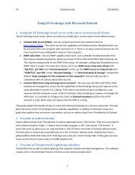
To test the effects of nonsatisfaction of Eq. (35), wehave
evaluated both sides of that equation with the KST2 functionals
and parametrization, Eq. (41). The left-hand panel of Fig. 3
shows the values from the left-hand side (LHS) and the
difference between the right-hand side (RHS) and LHS values
(RHS-LHS) of Eq. (35) at both s = 0.2 and s = 0.5. The righthand
panel of that figure shows the same quantities evaluated
for enhancement factors of the same form as Eq. (41) but with
parameters defined by the zero-temperature orbital-free kinetic
energy functional of Tran and Wesolowski (TW) 27 (see Sec. IV
for parameter values). The difference (RHS-LHS) is small
for both functionals. Although that difference increases with
increasing s, one may expect that the second term in Eq. (32)
will be close to the proper entropic contribution Eq. (36) for this
pair of functionals. Note moreover, that despite the seemingly
smaller error of the TW parametrization, in fact KST2 does
better in actual calculations; again see Sec. IV. Eventually the
quality of an approximate functional is defined by the quality
of its prediction of the noninteracting free energy F s .
We remark that, in all cases, the LHS and the RHS of
Eq. (35) are not continuous functions of t at t ≈ t 0 (see
Appendix A), the point at which the two fits for t t 0 and
t t 0 are joined. Clearly at least the second derivative of
the fits presented in Appendix A has abrupt behavior at t 0 .
Apparently this technical issue traces to Perrot’s original fits. 16
So far it has not proved problematic but may need to be
addressed in the future.
Reference 28 showed that the simple combination of the
VW and Thomas-Fermi functionals provides total energies
and lattice parameters which are reasonably close (at least
for a few systems) to those obtained with the mcGGA kinetic
energy functional, though the latter functional is better justified
5
4.5
4
3.5
LHS, s=0.2
-(RHS-LHS)x10, s=0.2
LHS, s=0.5
-(RHS-LHS)x10, s=0.5
3
2.5
2
1.5
1
0.5
0
0.01 0.1
t
1 10
3.5
3
2.5
2
1.5
1
0.5
LHS, s=0.2
-(RHS-LHS)x10, s=0.2
LHS, s=0.5
-(RHS-LHS)x10, s=0.5
0
0.01 0.1
t
1 10
FIG. 3. Left: LHS and RHS-LHS of Eq. (35) evaluated for KST2
enhancement factors, Eq. (41), ats = 0.2 and0.5. Right: Same
as left panel, but evaluated for enhancement factors Eq. (41) with
parameters defined by the Tran-Wesolowski (TW) kinetic energy
functional (Ref. 27).
115101-5

KARASIEV, SJOSTROM, AND TRICKEY PHYSICAL REVIEW B 86, 115101 (2012)
formally. Put into ftGGA form, the VWTF kinetic energy has
the enhancement factors
Fτ
VWTF (s τ ) = 1 + 5 3 s2 τ
F VWTF
σ (s σ ) = 1 − 5 3 s2 σ .
(42)
Thus we have the corresponding free energy functional
Fs
VWTF [n,T ] defined by Eqs. (32) and (42). AtT = 0K,this
is simply a rearrangement which exposes the TF contribution
as the choice of approximation for the so-called Pauli term, 12
while at T>0, the T -dependent Thomas-Fermi contribution
becomes the finite-T version.
III. IMPLEMENTATION
In Sec. I we remarked that OF-DFT in a plane-wave basis
(or on a numerical grid) requires a local pseudopotential (LPP)
(sometimes known as a regularized potential, depending on the
analysis used for development). Since it is desirable to exploit
the OF-DFT optimization tools in our modified version of the
ground-state PROFESS code, 29,30 the issue is germane here.
Perhaps the simplest form of regularization is the model
potential proposed by Heine and Abarenkov. 31,32 In real space,
it is
{ −A, r < rc
v mod (r) =
, (43)
−Z/r, r r c
where A is a constant, r c is the core radius, and Z is the core
charge. For use in a plane-wave code, it is convenient to have
a reciprocal space representation,
v mod (q) = −4π
Vq [(Z − Ar c)cos(qr 2 c )
+ (A/q)sin(qr c )]f (q), (44)
where V is the unit cell volume. The factor f (q) =
exp[(−q/q c ) 6 ] is a rounded step function introduced to
suppress spurious oscillations in v mod (q) caused by the Fourier
transform of the discontinuity of the real-space potential at
the core radius. This smoothing also ensures rapid decay
of v mod (q) at large wave vectors (see Ref. 31). In the work
reported below, we chose q c as suggested in that reference,
namely, to equal the position of the second zero of v mod (q).
For this initial study, we focus on hydrogen. For the H atom
we chose r c = 0.25 Bohr in Eq. (43), with the parameter A
determined by constraining a KS calculation with the local
pseudopotential (LPP) Eq. (43) to reproduce the reference
optimized simple-cubic hydrogen (sc-H) lattice constant a =
1.447 Å (see Table I). Those KS calculations were done
with Perdew-Zunger (PZ) LDA exchange-correlation 33 in the
ABINIT code. 34 KS reference calculations were performed with
the nonlocal projector augmented wave (PAW) scheme as
implemented in ABINIT using cutoff radius r c = 0.45 Bohr.
Both the ABINIT PAW and local (model) pseudopotential
calculations used an 8-atom unit cell and a 13 × 13 × 13 k
mesh. For further reference, corresponding bare potential
calculations were done with QUANTUM-ESPRESSO 35 using a
500 Ry energy cutoff and exactly the same unit cell and k
mesh.
TABLE I. Upper panel: Kohn-Sham equilibrium lattice constant
a (Å) and bulk modulus B (GPa) for sc-H calculated with QUANTUM-
ESPRESSO plane-wave code (PW) and bare Coulomb potential and
with ABINIT PW projector augmented wave (PAW) and model
potentials (real and reciprocal space). Lower panel: Comparison of
OF-DFT calculations using ftGGA(KST2), ftGGA(TW), ftVWTF,
and ftSGA noninteracting free-energy functionals in combination
with zero-temperature PZ LDA exchange correlation (Ref. 33) with
local pseudopotentials v mod (see text). All calculations are done at
electronic temperature T = 100 K (ionic temperature T ion = 0K).
See text regarding blank entries.
Method PP a B
Kohn-Sham
PW (QE) bare Coul. 1.446 108.4
PW (ABINIT) PAW 1.447 108.3
Kohn-Sham
PW (ABINIT) model a 1.447 108.1
PW (ABINIT) model reg. b 1.446 108.3
OF-DFT
ftGGA(KST2) model c 1.392 146
ftVWTF model c 1.394 146
ftGGA(TW) model c
ftSGA
model c
ftTF
model c
a Real space potential defined by Eq. (43).
b Real space potential defined by inverse Fourier-Bessel transform of
Eq. (44).
c Reciprocal space potential defined by Eq. (44).
The optimized parameter values which result are A =
6.18 Hartree, q c = 29.97 Bohr −1 . Figure 4 shows both the
original real-space and the back-transformed potential (after
reciprocal-space smoothing) for hydrogen.
Figure 5 gives a comparison of pressures calculated from
the model potential (again with ABINIT) and the bare Coulomb
potential (with QUANTUM-ESPRESSO) for standard KS calculations
on sc-H at two temperatures, 100 and 100 000 K,
again with simple PZ LDA. Since we are interested only in
v (Hartree)
−1
−2
−3
−4
−5
−6
−7
model
model reg.
0 0.1 0.2 0.3 0.4 0.5 0.6 0.7
r (Bohr)
FIG. 4. Model pseudopotential for hydrogen in real space as
defined by Eq. (43) and the smoothed version which results from
inverse Fourier-Bessel transform of v mod (q), Eq. (44).
115101-6

GENERALIZED-GRADIENT-APPROXIMATION ... PHYSICAL REVIEW B 86, 115101 (2012)
P (GPa)
10000
1000
100
KS (bare Coulomb) T=100 K
KS (bare Coulomb) T=100 000 K
KS (LPP) T=100 K
KS (LPP) T=100 000 K
Total free energy per atom (eV)
0.2
0.1
KS (LPP)
ftVWTF
ftGGA(KST2)
ftSGA
ftGGA(TW)
ftTF
10
5 10 15
ρ H
(g/cm 3 )
FIG. 5. (Color online) Test of model potential Eq. (44) for
sc-H by comparison between Kohn-Sham results obtained with
the bare Coulomb nuclear-electron interaction and those obtained
with Eq. (44) (both with PZ LDA XC functional) for T = 100 and
100 000 K.
the effects of regularization, the deficiencies of ground state
LDA-XC as an implicitly temperature-dependent functional
are irrelevant. For both electronic temperatures, the pressure
from the local (regularized) pseudopotential calculations is
in excellent agreement with results from the bare Coulomb
nuclear-electron potential calculations. The total free energies
from these two calculations also are in near-perfect agreement:
The relative difference between the model potential and the
bare Coulomb results does not exceed 0.5% except for a small
range of material densities around ρ H ≈ 6g/cm 3 for both
temperatures, where the absolute value of the total free energy
is close to zero as it crosses from positive to negative values.
The upper part of Table I gives a detailed comparison of the
equilibrium KS predictions from these various potentials.
0
0.3 0.4 0.5 0.6 0.7 0.8
ρ H
(g/cm 3 )
FIG. 6. (Color online) Total free energy per atom as a function of
material density for sc-H at electronic temperature T = 100 K (ionic
temperature T ion = 0 K) for LPP KS and OF-DFT calculations (both
with PZ LDA XC functional). The LPP is Eq. (44).
Figure 6 compares Kohn-Sham and OF-DFT results for
total free energies per atom as a function of material density for
sc-H at electronic temperature T = 100 K. Both calculations
were done with the same regularized local potential, Eq. (44).
The PROFESS OF-DFT calculation used a 64-atom supercell.
The KS calculations with local pseudopotential used an 8-atom
cell and a 13 × 13 × 13 k mesh. Two functionals, ftVWTF and
ftGGA(KST2), demonstrate reasonable agreement with the
KS reference data. As is evident from that figure, the widely
used ftSGA and ftTF functionals, as well as the ftGGA(TW)
functional, do not predict energy minima, at least in the range
of densities treated. The lower part of Table I shows OF-DFT
results for the equilibrium lattice constant and bulk moduli
obtained by fitting the calculated total energies per cell to
the stabilized jellium model equation of state (SJEOS). 36 Two
functionals, ftGGA(KST2) and ftVWTF, predict quite similar
results: The lattice constant is underestimated by three percent,
IV. OF-DFT RESULTS
All our OF-DFT calculations were done with a locally
modified version of the PROFESS code. 29,30 For simplicity
and to provide a uniform, clear-cut comparison, all the
noninteracting free energy functionals we studied were used
in conjunction with the ground state PZ LDA exchangecorrelation
functional. 33
We implemented the new ftGGA functionals, Eq. (32),
with the enhancement factors defined in Eq. (41) Fτ KST2 ,
Fσ
KST2 [ftGGA(KST2)]. For comparison we also implemented
the ftVWTF functional, Fτ
VWTF , Fσ
VWTF ,fromEq.(42), and
the ftGGA version of the zero-temperature GGA kinetic
energy functional parameterized by Tran and Wesolowski
(TW). 27 The ftGGA(TW) enhancement factors have the form
of Eq. (41) but with C 1 = 0.2319 and a 1 = 0.2748. (In fairness
to those authors, the TW parameters were not intended for
this purpose.) For reference, we also implemented the familiar
finite-temperature TF and ftSGA free energy functionals in the
form of Eq. (32), where F τ = F σ = 1 for ftTF and F τ , F σ are
defined through Eq. (37) for ftSGA. To our knowledge, the only
noninteracting free-energy functionals proposed previously
are these last two, ftTF and ftSGA.
F (per atom, eV)
-10
-11
-12
-13
-14
-15
-16
-17
-18
-19
KS(LPP) ρ H =2.0 g/cm 3
-20
ftVWTF
ftGGA(KST2)
ftSGA
-21 ftGGA(TW)
ftTF
-22
0 1020304050 60 70 80 90100
T (kK)
100
(%)
10
1
ρ H
=2.0 g/cm 3
ftVWTF
ftGGA(KST2)
ftSGA
ftGGA(TW)
ftTF
0.1
0.1 1 10
T (kK)
100 1000
FIG. 7. (Color online) Left: total free-energy per atom as a function
of electronic temperature for LPP KS and OF-DFT calculations
(both with PZ LDA XC functional). Right: relative free energy
differences with respect to KS values, |(F s − Fs
KS )/Fs KS |×100%
for the ftVWTF, ftGGA(KST2), ftSGA, ftGGA(TW), and ftTF free
energy functionals. Material density ρ H = 2.0 g/cm 3 .TheLPPis
Eq. (44).
115101-7

KARASIEV, SJOSTROM, AND TRICKEY PHYSICAL REVIEW B 86, 115101 (2012)
-5
100
1500
-6
1000
100
F (per atom, eV)
-7
-8
-9
-10
-11
KS(LPP) ρ H =4.0 g/cm 3
ftVWTF
-12
ftGGA(KST2)
ftSGA
ftGGA(TW)
ftTF
-13
0 1020304050 60 70 80 90100
T (kK)
(%)
10
1
ρ H
=4.0 g/cm 3
ftVWTF
ftGGA(KST2)
ftSGA
ftGGA(TW)
ftTF
0.1
0.1 1 10
T (kK)
100 1000
FIG. 8. (Color online) As in Fig. 7 for ρ H = 4.0g/cm 3 .
but the bulk modulus is overestimated by about 40%. These
results are encouraging as compared to the other three orbitalfree
functionals.
The left-hand panels of Figs. 7 and 8 compare Kohn-Sham
and OF-DFT total free energies per atom as a function of
electronic temperature for two material densities, ρ H = 2.0 and
4.0 g/cm 3 . The right-hand panels show relative differences of
the OF-DFT values with respect to the Kohn-Sham reference
results. At lower temperatures two functionals, ftVWTF and
ftGGA(KST2), overestimate the total free energy by about
10% and 15% for ρ H = 2.0 and 4.0 g/cm 3 , respectively. Two
functionals, ftSGA and ftGGA(TW), underestimate the free
energy with relative error between 20% and 30% for those
two densities. The error of the ftTF functional is much higher,
40% and 65%, respectively. It is interesting that the relative
error of all functionals remains nearly constant up to T =
100 000 K, after which that error decreases with increasing T .
At T = 1 000 000 K, the relative error of the ftTF functional
is about 0.4% and 1% for the two densities respectively, i.e.,
the high-temperature Thomas-Fermi limit is reached at this
1000
P (GPa)
200
100
60
KS (LPP) T=50 000 K
ftVWTF
ftGGA(KST2)
ftSGA
ftGGA(TW)
ftTF
0.6 0.8 1 1.2 1.4 1.6 1.8 2
ρ H
(g/cm 3 )
P (TPa)
95
90
85
KS (LPP) T=50 000 K
ftVWTF
ftGGA(KST2)
ftSGA
ftGGA(TW)
ftTF
18 18.5 19 19.5 20
ρ H
(g/cm 3 )
FIG. 10. (Color online) As in Fig. 9 for electronic temperature
T = 50 000 K.
point. Also we note that for T>200 000 K ( ρ H = 2.0g/cm 3 )
and T>400 000 K (ρ H = 4.0 g/cm 3 ), the relative errors of
the ftSGA and ftGGA(TW) functionals become smaller than
the errors of the ftVWTF and ftGGA(KST2). This behavior
may be understood by the fact that for those temperatures
the system may be considered as a weakly inhomogeneous
gas before reaching the high-T Thomas-Fermi limit. In
such circumstances, the second-order gradient approximation
should be appropriate.
Figures 9–11 compare KS and OF-DFT results for pressure
versus material density in sc-H at electronic temperatures
T = 100, 50 000, and 100 000 K, respectively. At low
temperature, the functionals clearly fall into two groups at the
lower densities. The ftGGA(KST2) and ftVWTF functionals
give slightly low pressures compared to the KS result, while the
pure ftTF, ftSGA, and ftGGA(TW) functionals yield distinctly
higher pressures. For the higher densities, the pressures from
all the functionals become closer (as they should, since ftTF
is the eventual limit). Similarly, the pressures from all the
functionals are closer at T = 50 000 and 100 000 K, but two
100
2000
105
95
100
P (GPa)
100
KS (LPP) T=100 K
ftVWTF
ftGGA(KST2)
ftSGA
ftGGA(TW)
ftTF
10
0.6 0.8 1 1.2 1.4 1.6 1.8 2
ρ H
(g/cm 3 )
P (TPa)
90
85
KS (LPP) T=100 K
ftVWTF
ftGGA(KST2)
ftSGA
ftGGA(TW)
ftTF
18 18.5 19 19.5 20
ρ H
(g/cm 3 )
FIG. 9. (Color online) Pressure as a function of material density
(low to intermediate at left, high at right) for sc-H at electronic
temperature T = 100 K for LPP KS and OF-DFT calculations (both
with PZ LDA xc functional). The LPP is Eq. (44).
P (GPa)
1000
KS (LPP) T=100 000 K
300
ftVWTF
ftGGA(KST2)
ftSGA
ftGGA(TW)
ftTF
200
0.6 0.8 1 1.2 1.4 1.6 1.8 2
ρ H
(g/cm 3 )
P (TPa)
95
90
85
KS (LPP) T=100 000 K
ftVWTF
ftGGA(KST2)
ftSGA
ftGGA(TW)
ftTF
18 18.5 19 19.5 20
ρ H
(g/cm 3 )
FIG. 11. (Color online) As in Fig. 9 for electronic temperature
T = 100 000 K.
115101-8

GENERALIZED-GRADIENT-APPROXIMATION ... PHYSICAL REVIEW B 86, 115101 (2012)
functionals from the first group [ftGGA(KST2) and ftVWTF]
yield visibly smaller errors compared to the second group for
all density ranges and for all electronic temperatures, with one
exception, ftSGA. It separates itself from the former second
group at T = 100 000 K and gets closer to the KS behavior
in a small range of densities (approximately 0.6–1.2 g/cm 3 )
than at lower temperatures. At T = 50 000 K and for low
densities, the relative error of the first group of functionals
[ftSGA, ftGGA(TW), and ftTF] is between 30% and 50%,
while the relative error from the ftGGA(KST2) and ftVWTF
functionals is about 30%. With increasing temperature, for low
densities all the functionals give pressures closer to the KS
results. At T = 100 000 K, the errors for ftGGA(KST2) and
ftSGA are about 7%. At high density for all temperatures, the
relative error of the ftGGA(KST2) functional is less than 1%,
while the error of functionals from the first group is between
1% and 2%.
Finally, we return to the issue of positivity of the entropy
for the KST2 functional. Equation (35) may be rearranged to
the form
∫ [
TS s := − ξ ′ (t)F τ (s τ ) − ξ(t)F τ ′ (s τ ) ∂s τ
∂t
+ ζ ′ (t)F σ (s σ ) + ζ (t)F σ ′ (s σ ) ∂s σ
∂t
− 1 ]
t ζ (t)F σ (s σ ) tτ0 TF (n)dr. (45)
By comparison with Eqs. (36) and (32), we recognize
immediately that Eq. (45) gives the difference between the
GGA entropy defined in Eq. (36) and the entropic contribution
from the approximate functional given by the second term in
Eq. (32). IfEq.(35) is satisfied exactly, then the bracket in
Eq. (45) is zero, hence TS s = 0. Thus we have two ways of
assessing the proper behavior of a proposed entropy functional.
Table II shows that, at least for the sc-H system, the KST2
GGA enhancement factor defined by Eqs. (41) gives a properly
positive entropy. There is little or no contamination by negative
contributions relative to the total T S s value. For material
densities at least as low as 0.5 g/cm 3 and higher, the negative
contribution to the entropy is zero. Moreover, the deviation
from satisfaction of Eq. (35) is small compared to the entropy,
that is, |TS s |/TS s ≈ 0. This is not true for a ftGGA based
on a different zero-temperature ofKE functional, as illustrated
by the results for ftGGA(TW) in that table. Nevertheless, the
behavior of TS s with increasing temperature is similar for
both functionals. Also, the SGA entropy is positive, not an
entirely expected result in view of the fact that the SGA
enhancement factor Fσ SGA (s σ ) can go negative, recall Eq. (37).
V. SUMMARY AND CONCLUSIONS
We have presented an analytical route for the development
of finite-temperature analogs of the GGA for the
noninteracting free-energy functional, as well as a simplified
version of it. Analysis of the finite-temperature second-order
gradient expansion of the free energy leads to the definition
of temperature-dependent reduced density gradients for both
the kinetic and entropic contributions to the free energy. The
dependence of these variables upon reduced temperature t
is smooth and they have proper t ≪ 1 and t ≫ 1 behavior.
We comment that, in principle one may try to use the
gradient expansion for the total noninteracting free energy
Eq. (27) to define a corresponding temperature-dependent
reduced density gradient s f , then introduce a ftGGA with
a single enhancement factor F f (s f ). But it becomes clear
almost immediately that the variable sf 2 is not positive definite.
Moreover, it has a pole because the function κ(t), which
appears in the denominator of the variable s f , has a zero
(see Fig. 1). This analysis leads to the conclusion that a
finite-T GGA should be constructed with the kinetic and
entropic contributions treated separately (as we have done),
not combined in a functional with a single enhancement factor.
Such a two-part ftGGA functional is defined completely
by a pair of enhancement factors, F τ and F σ . From standard
thermodynamics, it follows that these enhancement factors
are not independent. We have given the formal relationship
in Eq. (35), but the solution of that equation relating F τ
and F σ is formidable. As an initial step therefore, we have
proposed a simpler approximate relationship between the two
enhancement factors and showed that it provides reasonably
TABLE II. Noninteracting entropic component of the free-energy functional T S s , negative contribution T Ss − , and the difference between
Eq. (36) and the second term of Eq. (32) for the ftGGA functionals for 1-atom sc-H at density ρ H = 0.15 g/cm 3 and ionic temperature
T ion = 0 K. All in eV.
ftVWTF ftGGA(KST2) ftSGA ftGGA(TW)
T(K) T S s T S − s
T S s T S − s
TS s T S s T S − s
T S s T S − s
TS s
5 000 0.10 0.0 0.10 0.0 0.0 0.10 0.0 0.10 −0.01 −0.01
10 000 0.40 0.0 0.38 0.0 −0.01 0.37 0.0 0.38 −0.02 −0.03
20 000 1.47 0.0 1.48 −0.01 −0.02 1.37 0.0 1.41 −0.07 −0.09
30 000 3.30 0.0 3.32 −0.01 −0.03 2.91 0.0 3.00 −0.12 −0.15
40 000 5.78 0.0 5.85 0.0 −0.02 4.88 0.0 4.98 −0.17 −0.21
50 000 8.69 0.0 8.78 0.0 −0.01 7.23 0.0 7.35 −0.19 −0.25
100 000 26.36 0.0 26.42 0.0 0.0 23.00 0.0 23.1 −0.3 −0.4
250 000 95.11 0.0 95.14 0.0 0.0 93.05 0.0 91.1 −0.3 −0.5
300 000 121.15 0.0 121.18 0.0 0.0 119.69 0.0 117.4 0.0 −0.4
400 000 176.33 0.0 176.36 0.0 0.0 175.40 0.0 174.7 0.0 −0.1
1 000 000 559.03 0.0 559.05 0.0 0.0 558.77 0.0 558.8 0.0 −0.0
115101-9

KARASIEV, SJOSTROM, AND TRICKEY PHYSICAL REVIEW B 86, 115101 (2012)
ν(t)
2.5
2
1.5
1
0.5
0
0.01 0.1 1 10
FIG. 12. ν(t) as defined by Eq. (B2).
satisfactory results. In the T → 0 limit, all ftGGA free energy
functionals should reduce to known zero-temperature kinetic
energy functionals, a fact we have used to present a rather
simple ftGGA.
Numerical implementation of the OF-DFT calculations in
a plane-wave basis requires a local pseudopotential which we
have presented. Comparison of finite temperature OF-DFT
and KS calculations on sc-H over a wide range of material
densities for electronic temperatures up to 100 000 K leads to
the conclusions that two ftGGA functionals, namely KST2
and VWTF, provide the overall best results and that the
relative error in the high density regime is small for all
functionals.
ACKNOWLEDGMENTS
We acknowledge informative conversations with Frank
Harris and Jim Dufty with thanks. This work was supported
in substantial part by the US Dept. of Energy TMS Grant No.
DE-SC0002139.
APPENDIX A
The temperature scaling function κ introduced in Eq. (16)
may be written by use of Eqs. (9) and (15) as
t
) −5/3
κ(βμ) = 5 ( 3
2 2 I 1/2(βμ)
[
× − 2 ]
3 I 3/2(βμ) + βμI 1/2 (βμ) . (A1)
By use of Eq. (14), we may eliminate (βμ) infavoroft
in Eq. (A1). We have done that numerically. With that result,
we can present κ(t) analytically as an adapted form of Perrot’s
free energy fit. 16 See below. The functions ζ (t) and ξ(t) may
be calculated using relations with κ(t) giveninEqs.(18)
and (19). In addition, we provide an adapted analytical ˜h(t).
Both functions are split into regions t t 0 and t t 0 , where
t 0 = 4(2/3π 2 ) 1/3 /3, to take account of the different asymptotic
forms of the Fermi integrals for (βμ) ≪ 0 and (βμ) ≫ 0.
For t t 0 = 0.543010717965,
κ(t) =−2.5t ln(t) − 2.141088549t + 0.2210798602t −0.5
+ 0.7916274395 × 10 −3 t −2 − 0.4351943569
× 10 −2 t −3.5 + 0.4188256879 × 10 −2 t −5
− 0.2144912720 × 10 −2 t −6.5 + 0.5590314373
× 10 −3 t −8 − 0.5824689694 × 10 −4 t −9.5 (A2)
˜h(t) = 3 − 0.7996705242t −1.5 + 0.2604164189t −3
− 0.1108908431t −4.5 + 0.6875811936 × 10 −1 t −6
− 0.3515486636 × 10 −1 t −7.5 + 0.1002514804
× 10 −1 t −9 − 0.1153263119 × 10 −2 t −10.5 . (A3)
For t t 0 = 0.543010717965,
κ(t) = 1 − 4.112335167t 2 + 1.995732255t 4 + 14.83844536t 6
− 178.4789624t 8 + 992.5850212t 10 − 3126.965212t 12
+ 5296.225924t 14 − 3742.224547t 16 (A4)
˜h(t) = 1 + 3.210141829t 2 + 58.30028308t 4 − 887.5691412t 6
+ 6055.757436t 8 − 22429.59828t 10 + 43277.02562t 12
− 34029.06962t 14 .
APPENDIX B
(A5)
We outline a route to simplified GGAs which is a potential
alternative to the one given in the discussion of Eqs. (37)–(39).
Equations (37) obviously combine to give
Fσ SGA (s σ ) = 2 + 5 (
s
2
27 τ − sσ 2 )
− F
SGA
τ (s τ ). (B1)
As suggested in the discussion in conjunction with Fig. 2, the
ratio
ν(t) := [s σ (t)/s τ (t)] 2
(B2)
is a smooth, bounded [0 ν(t) 2.2] function. See Fig. 12.
With this function, Eq. (B1) becomes
F SGA
σ (s σ ) = 2 + 5
27 s2 τ
[1 − ν(t)] − F
SGA
τ (s τ ). (B3)
Utilization to form a GGA is via
Fσ GGA (s σ ) = 2 + 5
27 s2 τ [1 − νGGA (t)] − Fτ GGA (s τ ), (B4)
where the superscript “GGA” on ν indicates use of some
judiciously selected approximate representation of ν(t). This
choice can be constrained by insertion of the form from
Eq. (B4) in Eq. (35). We have this approach under study.
* vkarasev@qtp.ufl.edu
1 N. D. Mermin, Phys. Rev. 137, A1441 (1965).
2 M. V. Stoitsov and I. Zh. Petkov, Ann. Phys. 184, 121 (1988).
3 R. M. Dreizler, in The Nuclear Equation of State, Part A, edited
by W. Greiner and H. Stöcker, NATO ASI Vol. B216 (Plenum,
NY, 1989), p. 521.
115101-10

GENERALIZED-GRADIENT-APPROXIMATION ... PHYSICAL REVIEW B 86, 115101 (2012)
4 B.I.Dunlap,N.Rösch, and S. B. Trickey, Mol. Phys. 108, 3167
(2010).
5 J. P. Perdew, K. Burke, and M. Ernzerhof, Phys. Rev. Lett. 77, 3865
(1996); 78, 1396(E) (1997).
6 A. Vela, V. Medel, and S. B. Trickey, J. Chem. Phys. 130, 244103
(2009).
7 L. A. Constantin, E. Fabiano, S. Laricchia, and F. Della Sala, Phys.
Rev. Lett. 106, 186406 (2011).
8 J. M. del Campo, J. L. Gázquez, S. B. Trickey, and A. Vela, J.
Chem. Phys. 136, 104108 (2012).
9 J. P. Perdew, Phys. Lett. A 165, 79 (1992).
10 E. V. Ludeña and V. V. Karasiev, in Reviews of Modern Quantum
Chemistry: a Celebration of the Contributions of Robert Parr, edited
by K. D. Sen (World Scientific, Singapore, 2002), p. 612.
11 V. V. Karasiev, S. B. Trickey, and F. E. Harris, J. Comput.-Aided
Mat. Des. 13, 111 (2006).
12 V. V. Karasiev, R. S. Jones, S. B. Trickey, and F. E. Harris, Phys.
Rev. B 80, 245120 (2009).
13 L. H. Thomas, Proc. Cambridge Phil. Soc. 23, 542 (1927).
14 E. Fermi, Atti Accad. Nazl. Lincei 6, 602 (1927).
15 R. P. Feynman, N. Metropolis, and E. Teller, Phys. Rev. 75, 1561
(1949).
16 F. Perrot, Phys. Rev. A 20, 586 (1979).
17 J. W. Dufty and S. B. Trickey, Phys. Rev. B 84, 125118
(2011).
18 S. Pittalis, C. R. Proetto, A. Floris, A. Sanna, C. Bersier, K. Burke,
and E. K. U. Gross, Phys.Rev.Lett.107, 163001 (2011).
19 N. Troullier and J. L. Martins, Phys.Rev.B43, 1993 (1991).
20 N. A. W. Holzwarth, A. R. Tackett, and G. E. Matthews, Comput.
Phys. Commun. 135, 329 (2001).
21 P. E. Blöchl, Phys.Rev.B50, 17953 (1994).
22 E. Lieb, Rev. Mod. Phys. 48, 553 (1976).
23 J. Bartel, M. Brack, and M. Durand, Nucl. Phys. A 445, 263 (1985).
24 C. H. Hodges, Can. J. Phys. 51, 1428 (1973).
25 C. F. von Weizsäcker, Z. Phys. 96, 431 (1935).
26 M. Brack, C. Guet, and H.-B. Hakansson, Phys. Rep. 123, 275
(1985).
27 F. Tran and T. A. Wesolowski, Int. J. Quantum Chem. 89, 441
(2002).
28 V. V. Karasiev and S. B. Trickey, Comput. Phys. Commun. 183,
2519 (2012).
29 G. S. Ho, V. L. Lignères, and E. A. Carter, Comput. Phys. Commun.
179, 839 (2008).
30 L. Hung, C. Huang, I. Shin, G. S. Ho, V. L. Lignères, and E. A.
Carter, Comput. Phys. Commun. 181, 2208 (2010).
31 L. Goodwin, R. J. Needs, and V. Heine, J. Phys.: Condens. Matter
2, 351 (1990).
32 V. Heine and I. V. Abarenkov, Philos. Mag. 9, 451 (1964).
33 J. P. Perdew and A. Zunger, Phys. Rev. B 23, 5048
(1981).
34 X. Gonze et al., Comput. Phys. Commun. 180, 2582 (2009);
X. Gonze, G.-M. Rignanese, M. Verstraete, J.-M. Beuken,
Y. Pouillon, R. Caracas, F. Jollet, M. Torrent, G. Zerah, M. Mikami,
Ph. Ghosez, M. Veithen, J.-Y. Raty, V. Olevano, F. Bruneval,
L. Reining, R. Godby, G. Onida, D. R. Hamann, and D. C. Allan,
Z. Kristallogr. 220, 558 (2005).
35 Paolo Giannozzi et al., J. Phys.: Condens. Matter 21, 395502
(2009).
36 A. B. Alchagirov, J. P. Perdew, J. C. Boettger, R. C. Albers, and
C. Fiolhais, Phys. Rev. B 63, 224115 (2001).
115101-11