PDF Version

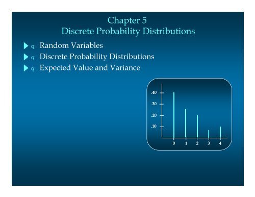
Chapter 5
Discrete Probability Distributions
■
■
■
Random Variables
Discrete Probability Distributions
Expected Value and Variance
.40
.30
.20
.10
0 1 2 3 4

Random Variables
A random variable is a numerical description of the
outcome of an experiment.
A discrete random variable may assume either a
finite number of values or an infinite sequence of
values.
A continuous random variable may assume any
numerical value in an interval or collection of
intervals.

Example: JSL Appliances
■
Discrete random variable with a finite number
of values
Let x = number of TVs sold at the store in one day,
where x can take on 5 values (0, 1, 2, 3, 4)

Example: JSL Appliances
■
Discrete random variable with an infinite sequence
of values
Let x = number of customers arriving in one day,
where x can take on the values 0, 1, 2, . . .
We can count the customers arriving, but there is no
finite upper limit on the number that might arrive.

Random Variables
Question Random Variable x Type
Family
size
Distance from
home to store
Own dog
or cat
x = Number of dependents
reported on tax return
x = Distance in miles from
home to the store site
x = 1 if own no pet;
= 2 if own dog(s) only;
= 3 if own cat(s) only;
= 4 if own dog(s) and cat(s)
Discrete
Continuous
Discrete

Discrete Probability Distributions
The probability distribution for a random variable
describes how probabilities are distributed over
the values of the random variable.
We can describe a discrete probability distribution
with a table, graph, or equation.

Discrete Probability Distributions
The probability distribution is defined by a
probability function, denoted by f(x), which provides
the probability for each value of the random variable.
The required conditions for a discrete probability
function are:
f(x) > 0
Σf(x) = 1

Discrete Probability Distributions
■
■
Using past data on TV sales, …
a tabular representation of the probability
distribution for TV sales was developed.
Number
Units Sold of Days
0 80
1 50
2 40
3 10
4 20
200
x f(x)
0 .40
1 .25
2 .20
3 .05
4 .10
1.00
80/200

Discrete Probability Distributions
■
Graphical Representation of Probability Distribution
.50
Probability
.40
.30
.20
.10
0 1 2 3 4
Values of Random Variable x (TV sales)

Discrete Uniform Probability Distribution
The discrete uniform probability distribution is the
simplest example of a discrete probability
distribution given by a formula.
The discrete uniform probability function is
f(x) = 1/n the values of the
random variable
are equally likely
where:
n = the number of values the random
variable may assume

Expected Value and Variance
The expected value, or mean, of a random variable
is a measure of its central location.
E(x) = μ = Σxf(x)
The variance summarizes the variability in the
values of a random variable.
Var(x) = σ 2 = Σ(x - μ) 2 f(x)
The standard deviation, σ, is defined as the positive
square root of the variance.

Expected Value and Variance
■
Expected Value
x f(x) xf(x)
0 .40 .00
1 .25 .25
2 .20 .40
3 .05 .15
4 .10 .40
E(x) = 1.20
expected number of
TVs sold in a day

Expected Value and Variance
■
Variance and Standard Deviation
E(x) = 1.20
x
x - μ (x - μ) 2 f(x) (x - μ) 2 f(x)
0
1
2
3
4
-1.2
-0.2
0.8
1.8
2.8
1.44
0.04
0.64
3.24
7.84
.40
.25
.20
.05
.10
.576
.010
.128
.162
.784
Variance of daily sales = σ 2 = 1.660
TVs
squared
Standard deviation of daily sales = 1.2884 TVs

Binomial Distribution
■
Four Properties of a Binomial Experiment
1. The experiment consists of a sequence of n
identical trials.
2. Two outcomes, success and failure, are possible
on each trial.
3. The probability of a success, denoted by p, does
not change from trial to trial.
stationarity
4. The trials are independent. assumption

Binomial Distribution
Our interest is in the number of successes
occurring in the n trials.
We let x denote the number of successes
occurring in the n trials.

Binomial Distribution
■
Binomial Probability Function
n
!
x
f ( x ) = p (1 −
p
)
x !( n
−
x
)!
( n −
x
)
where:
f(x) = the probability of x successes in n trials
n = the number of trials
p = the probability of success on any one trial

Binomial Distribution
■
Binomial Probability Function
n
!
x
f ( x ) = p (1 −
p
)
x !( n
−
x
)!
( n −
x
)
n
!
x !( n
−
x
)!
Number of experimental
outcomes providing exactly
x successes in n trials
x
p (1 p )
−
( n x
−
)
Probability of a particular
sequence of trial outcomes
with x successes in n trials

Binomial Distribution
■
Example: Evans Electronics
Evans is concerned about a low retention rate for
employees. In recent years, management has seen a
turnover of 10% of the hourly employees annually.
Thus, for any hourly employee chosen at random,
management estimates a probability of 0.1 that the
person will not be with the company next year.

Binomial Distribution
■
Using the Binomial Probability Function
Choosing 3 hourly employees at random, what is
the probability that 1 of them will leave the company
this year
f ( x
)
=
Let: p = .10, n = 3, x = 1
n
!
p
x !( n
−
x
)!
x
n x
( p) ( −
1−
)
3!
f = = =
1!(3 −
1)!
1 2
(1) (0.1) (0.9) 3(.1)(.81) .243

Binomial Distribution
■
Using Tables of Binomial Probabilities
p
n
x .05 .10 .15 .20 .25 .30 .35 .40 .45 .50
3 0 .8574 .7290 .6141 .5120 .4219 .3430 .2746 .2160 .1664 .1250
1 .1354 .2430 .3251 .3840 .4219 .4410 .4436 .4320 .4084 .3750
2 .0071 .0270 .0574 .0960 .1406 .1890 .2389 .2880 .3341 .3750
3 .0001 .0010 .0034 .0080 .0156 .0270 .0429 .0640 .0911 .1250

Binomial Distribution
■
Expected Value
E(x) = μ = np
■
Variance
Var(x) = σ 2 = np(1 − p)
■
Standard Deviation
σ =
np
(1 −
p
)

Binomial Distribution
■
Expected Value
E(x) = μ = 3(.1) = .3 employees out of 3
■
Variance
Var(x) = σ 2 = 3(.1)(.9) = .27
■
Standard Deviation
σ = 3(.1)(.9) =
.52 employees