Solving Kepler's Problem Mechanically - Scientific Instrument Society

Solving Kepler’s Problem Mechanically
Martin Beech
Introduction
There are occasions when it is tempting
to think that there might be such an entity
as the ecology of scientific instruments.
Specialist measuring and analysis devices
appear, just like new animal species, when
there is a specific niche to be filled, and just
as animal species can become extinct and
overrun, so too can the specialist scientific
instrument be replaced and made obsolete.
Indeed, we only know of the past existence
of some instruments because of the ‘fossil
record’ that they have left behind, buried
deep within the ancient and often obscure
scientific literature.
I am aware of only one instrument directly
constructed for the mechanical solution of
Kepler’s problem having survived into the
modern era (to be described below). There
were probably very few such instruments
constructed in the first place, and for the
best part of the last half-a-century their
specific application has not been required.
Indeed, they have been replaced, as have so
many mechanical and analog devices of the
past, by the electronic computer which can
obtain the required results more rapidly and
with much greater numerical accuracy. To
my knowledge the machines for solving Kepler’s
problem have no specific name, and
while a number of variant designs for such
devices have seen publication in the astronomical
literature, they can all be thought
of as analogue computers. From a practicing
astronomy perspective, the heyday for
the application of such devices spanned an
approximate 60-year time interval centered
on 1900. The initial appearance of these devices
was the result of a growing interest
in the study of binary star systems and the
analysis of cometary and asteroid orbits; at
issue was the determination of the position
of a star, comet or asteroid within its orbit
as a function of time and orbital eccentricity.
This particular problem has a solution
in the form of Kepler’s equation, which
describes the mathematical relationship
between the orbital eccentricity, the mean
anomaly, and the eccentric anomaly.
Kepler’s Problem and a Potted History
of How to Solve it
There is a long history behind the solution
of Kepler’s problem 1 , and it is a very good
example of how difficult it can sometimes
be to find a solution to what is in all reality
a harmless enough looking equation. At
stake is the solution of the equation for E
when M and e are specified:
M = E – e. sin E (1)
The symbols entering equation (1) are the
eccentric anomaly E, the eccentricity e of
the orbit and the mean anomaly M. For any
given binary star system, comet or asteroid
orbit the eccentricity will be a fixed
value, with 0 e < 1, but the mean anomaly
M will vary between 0 and 2 during
one complete orbit. The mean anomaly is,
therefore, the time variable term and it is
defined as M = t (2 / P), where t is the
time and P is the orbital period. 2 Solutions
to (1) will return values for the eccentric
anomaly in the range 0 E 2. At issue
with equation (1), and the very basis
of Kepler’s problem, is that it admits of no
analytic solutions 3 for E – the equation is
said to be transcendental. The manner in
which a solution can be found, however, as
Kepler initially discovered 1 , is to assume an
initial starting value E 0
and then work by
substitution and repeated iteration with
E n+1
= E n
+ E , n = 0, 1, 2, 3…., until the
correction E becomes so small that it
can be safely ignored. 4 Mathematically this
presupposes that a solution actually exists
and that convergence will occur – but this
is another problem. 1 In the modern era a
simple computer subroutine can find a solution
to equation (1) very rapidly using a
Newton-Raphson iteration scheme. In years
past, however, the situation was much less
straightforward, more time-consuming and,
of course, any calculations had to be done
by hand. Such circumstances typically result
in the design and construction of mathematical
tables, graphical methods and/or
analog compute devices, and this was exactly
the case with Kepler’s problem. Indeed,
within his classic textbook Celestial
Mechanics, published in 1953, Professor
William M. Smart (University of Glasgow)
makes the comment, ‘a value may be obtained
by one of many graphical methods
devised for this purpose – of which there
are about 120 – or means of special tables;
such tables give the values of M in Kepler’s
equation calculated for selected values of
E and e’. 5 Smart refers to two specific sets
of tables; one by Julius Bauschinger which
was published in Leipzig in 1901, the other
by J. J. Astrand, also published in Leipzig in
1890. Of the graphical methods developed
to solve Kepler’s problem the most commonly
employed scheme is that utilizing
the curve of sines. Professor Charles Young
(Princeton University) in his widely read
book A textbook of General Astronomy
for Colleges and Scientific Schools, first
published in 1889, describes one such
curve of sines method, but notes, ‘owing to
the slight imperfections in the diagram, in
the ruling of the squares, unequal shrinkage
of the paper, etc., the value of E obtained
from it are only approximate, but can generally
be relied on to within about ¼ o . This
is near enough for many purposes (double
star orbits for instance), and is always sufficient
as the starting point for a numerical
calculation.’
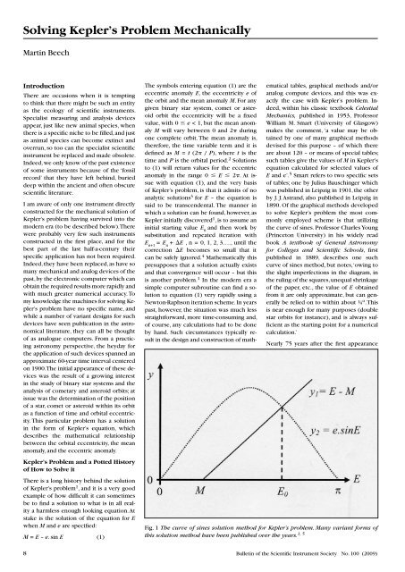
Nearly 75 years after the first appearance
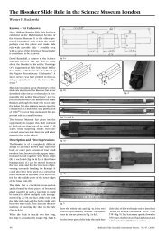
Fig. 1 The curve of sines solution method for Kepler’s problem. Many variant forms of
this solution method have been published over the years. 1, 5
8 Bulletin of the Scientific Instrument Society No. 100 (2009)

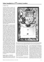
Fig. 2 Wren’s cycloid development solution to Kepler’s Problem – based upon the diagram
presented by Isaac Newton in his Principia Mathematica.
of Young’s book, Sidney W. McCuskey (Case
Institute of Technology) also provides a
curve of sines method in his text Introduction
to Celestial Mechanics (published in
1963). With reference to Fig. 1, McCuskey
explains, ‘let y 1
= E – M, and y 2
= e sin E.
Then we plot the two curves as shown [see
figure 1]’ with the first approximation to
the solution E 0
being read-off the x-axis at
the point of intersection of y 1
and y 2
. Once
E 0
has been found then a single iteration 4
should produce a highly accurate solution.
Variants of the solution method outlined
by McCuskey have also been published on
numerous other occasions, and a pseudomechanical
version of it, due to the Reverend
Charles Pritchard, will be discussed
below. It is interesting to note, however,
that even in the early 1960s, when McCuskey’s
text was first published the limited
access to electronic computing machines
still dictated the use of a graphical solution
approach.
When the orbital eccentricity is small various
power series solutions to equation (1)
can be developed. W. M. Smart, for example,
describes the solution method developed
by E. W. Brown (Yale University) which is
a truncated series expansion accurate to
terms of order O(e 6 ), and for which, when
e < 0.14, the error in E is less than 0.1 seconds
of arc. Numerous series solutions to
Kepler’s equation have been published 1 ,
with many of the most famous mathematicians
and astronomers of the 18 th and 19 th
centuries (including Adams, Bessel, Cassini,
Euler, Gauss, Lagrange, Laplace and Le Verrier)
contributing papers on the subject.
While an exhaustive search of the literature
has not been made, the earliest text that I
have been able to find in which a solution
method requiring the use of a ‘modern calculating
machine’ (by which a mechanical
calculating device is implied) is The Computation
of Orbits, published privately
by Paul Herget, of Cincinnati Observatory,
in 1948. The first text that I have found in
which a BASIC computer language subroutine
to solve Kepler’s equation is described
is Peter Duffett-Smith’s, Astronomy with
your personal computer, which was first
published in 1985. Duffett-Smith describes a
Newton-Raphson iteration scheme for solving
Kepler’s equation to an accuracy of order
10 -6 radians. Several BASIC subroutines
capable of solving Kepler’s equation were
also published in the revised and enlarged
1988 reissue of J. M. A. Danby’s, Elements of
Celestial Mechanics. In the first edition of
Danby’s text, published in 1962, however,
a slide rule and five-figure logarithm table
method for solving Kepler’s equation is described,
with the curve of sines method being
given only a brief mention.
Wren’s Solution Curve
The first geometrical solution to Kepler’s
problem was the cycloid development
method discovered by Sir Christopher
Wren in 1658. The scheme was first described,
however, by Oxford mathematician
the Reverend John Wallis in an appendix to
his De Cycloide, published in 1659 - there
triumphantly described under the title De
problemate Kepleriane per cycloidem solvendo.
We also note the intriguing account
in Robert Hooke’s diary 6 for Thursday, August
16 th in 1677, ‘At the Crown, Sir Christopher
told of killing the wormes with burnt
oyle and of curing his Lady of a thrush by
hanging a bag of live boglice about her
neck. Discoursed about the theory of the
Moon which I explained. Sir Christopher
told his way of solving Kepler’s problem
by the Cycloeid’. The ‘Crown’ is probably
the Crown Tavern in Threadneedle Street
which various members of the Royal Society
used to frequent 6 , and it does indeed
seem that the discourse between Hooke
and Wren covered a great range of topics.
Wren’s solution to Kepler’s problem is also
that presented by Sir Isaac Newton in Book
I, De Corpus Moto of his Principia (first
published in 1687). Fig. 2 is based upon the
diagram given by Newton in Proposition
XXXI (problem XXIII), and as Newton explains
6 , ‘in the ellipse APB let A be a main
vertex, S a focus, O the centre, and let P be
the body’s position needing to be found.’
With reference to Fig. 2, the basic idea of
Wren’s method is to extend the major axis
of the elliptical orbit APB to meet the horizontal
line HKG such that the distance OG
is to OA as OA is to OS. This process introduces
the eccentricity e into the solution
since by definition e = OS / OA. The circle
of radius OG is then ‘imagined’ to be rolled
along the horizontal HKG, with the cycloidal
arc ALI being accordingly generated.
The distance GK is then set-off according
to GK = M .OG, where 0 ≤ M ≤ 1 is the
mean anomaly. By erecting a perpendicular
at K to intercept the cycloid ALI at point L,
and then taking a horizontal from L to the
elliptical orbit APB, the intercept point P is
the location of the planet (star, comet or
asteroid) corresponding to the given mean
anomaly (M) and orbital eccentricity (e). An
interesting point about Wren’s solution is
that it is a purely geometric one and has
no physical attachment to the equations of
celestial mechanics. 7 In addition, as is often
the case with highly influential works such
as the Principia, a number of authors have
attributed the origin of the cycloidal solution
method to Newton rather than Wren.
The Development of an Idea
Astronomers working at Oxford University
appear to have been particularly interested
in and indeed, adept at inventing new mechanical
devices for solving Kepler’s problem.
The Savilian Professor of Astronomy,
Reverend Charles Pritchard writing in the
Monthly Notices of the Royal Astronomical
Society 8 for April, 1877 was, for example,
prompted to describe two mechanical
devices for solving Kepler’s equation after
the publication by Annibale de Gasparis
(in the March, 1877 issue of the Monthly
Notices) of a ‘simplified’, purely numerical
solution scheme. 9 Pritchard notes, ‘it is unnecessary
to dilate upon the boon which
would be conferred on observatories and
computers, if the tiresomeness of the solution
to this problem [Kepler’s problem]
Bulletin of the Scientific Instrument Society No. 100 (2009)
9

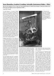
Fig. 3 The curve of sines slider and straightedge mechanical solution method for Kepler’s
problem. Image from ref. 8.
can be diminished’. 8 Indeed, the Gasparis
approach appears rather cumbersome (and
is not obviously a time-saving approach),
but as Pritchard comments every practitioner
has ‘his own peculiar method’. The
mechanical approach preferred by Pritchard
and indeed, the one ‘as used in the
Oxford University Observatory’ 8 is based
upon the curve of sines. The device is illustrated
here in Fig. 3. From the diagram,
KL is a groove that carries a slider attached
to which is an arm SR that swivels about
point O (labeled ‘fig. 4’ in the diagram). The
curve of sines runs along ADB and is constructed
on a scale such that the distance
A to B is 45 inches long and divided into
180 equal intervals. The distance CD =
14.324 inches and the distance DE = FE =
10 inches. The lines FE and DE are used to
set the slider arm SR with the line FE which
determines the orbital eccentricity. In the
illustration shown here the slider has been
set to represent and orbital eccentricity of
e = 0.875 (that is according to the chosen
scale being positioned 8.75 inches from E).
Having set the arm SR the thumbscrew at
O is tightened and the slider is moved so
that the edge of arm SR is located at the
specified mean anomaly (M = 124.933 degrees
in the example shown). Once located
at the position for M, the point U, at which
straightedge SR cuts the curve of sines, is
the desired eccentric anomaly E (with E =
150 degrees in the example given).
Pritchard claims that the device he has constructed
is accurate to 2 arc seconds, and
that, ‘the machine admits of home manufacture:
and … solves the question of Kepler’s
Problem with sufficient accuracy for
double-star orbits without further computation.’
Radcliffe Observer, Arthur A. Rambaut (1859
– 1923) 10 was a renowned mathematician,
graduating from Trinity College, Dublin
with its Gold Medal for Mathematics and
Mathematical Physics in 1881. Given this
background and training it is perhaps not
surprising that Rambaut developed and
constructed several new mechanical devices
for solving Kepler’s equation. His first
device 11 was described in March of 1890,
and is a mechanical development of Wren’s
method, although Rambaut appears (at that
time) to be unaware of the historical link.
Fig. 4 illustrates the author’s re-construction
of the method outlined by Rambaut. The
key mechanical (or moving) component is
a semi-circle cut from stiff card – simplicity
itself. The solution method does work well,
but great care has to be exercised in order
to avoid any slippage when rolling the semicircle
arc along the straight edge.
With reference to Fig. 4, the line MN corresponds
to a straight edge glued to the
graph paper. POQ is a vertical to MN. The
central axis line ROS is parallel to MN and
is divided so that the distance OS = 180-
mm is equivalent to 180 degrees (i.e. a scale
of 1-degree per one millimeter division of
graph paper). The distance PO between the
lines MN and ROCS (and also the radius of
the semi-circle CA) is set according to the
scale PO = 180 / = 57.3-mm. The focal
point of the orbit to be studied is located at
F, with CF / CA = e. In the example shown
in figure 4, the mean anomaly is taken as M
= 120 o , and accordingly the diameter of the
right-most semi-circle is aligned vertically
to MN at this reading. The eccentricity is
taken to be e = 0.75 (shown by the small
Fig. 4 The author’s re-construction of Rambaut’s rolling semi-circle method for solving
Kepler’s problem. The background is a standard letter-sized piece of graph paper ruled
with 1-mm divisions. The central axis ROCS has a scale of 1 degree per millimeter, which
dictates that the diameter of the semi-circle is 360 / = 114.6-mm. The figure shows
the cycloid produced when the eccentricity is e = 0.75. Note, the stiff-card semi-circle has
been replaced in this image by two partially transparent cut-outs at the starting and
end points of the ‘calculation’.
10 Bulletin of the Scientific Instrument Society No. 100 (2009)

Fig. 5 Rambaut’s second method for mechanically solving
Kepler’s equation. The circle with centre C can be of any
radius. The arc AM corresponds to the angle of the mean
anomaly M, and the locus MVT is the involute arc drawn
from point M. The radius AC is divided at F so that the
ratio FC / AC = e, the orbital eccentricity. The line QFPV is
drawn through F forming a tangent to the involute at V.
The angle AFV (which is also equal to angle ACU) is the
required solution for E.
circle at F). The curved edge of the semicircle
is rolled along MN until the point F
just touches the vertical POQ (shown by
the leftmost semi-circle). The required solution
to Kepler’s equation is now determined
as the sum E = M + OC’, and from
the graph paper OC’ = 24.5 o , indicating that
E = 144.5 o . An exact numerical solution for
the chosen values gives E = 144.78 degrees,
suggesting that an accuracy of about ¼ of a
degree (15 arc minutes) might reasonably
be expected from Rambaut’s device.
Rambaut described a second mechanical
device 12 for solving Kepler’s problem in
June of 1906. His new method employed
an involute of the circle development (Fig.
5) and Rambaut argued that the device was
able to provide solutions to ‘within onetenth
of a degree in elliptical orbits of any
eccentricity’. Rambaut enlisted the talents
of Henry Minn, ‘a skilful watchmaker’ in
the construction of a working version his
instrument (which is now held within the
collection of the Museum of the History
of Science at Oxford). A full description of
Rambaut’s device will appear in a subsequent
article. As far as I am aware the device
at Oxford is the only extant analogue
machine specifically constructed to solve
Kepler’s problem.
As with his first publication on the mechanical
solution to Kepler’s problem, Rambaut
was prompted to describe his new invention
in response to an earlier
article on the topic 13 , this
time by Thomas Jefferson
Jackson See, of the University
of Chicago. See was again motivated
to seek solutions to
Kepler’s problem as a result
of an interest in binary star,
asteroid and cometary orbit
analysis, arguing, ‘it seems
clear that a general method
for solving Kepler’s equation
by mechanical means
is an urgent desideratum of
astronomy.’ See’s approach,
as Rambaut noted, is little
more than a slight variant
of Pritchard’s curve of sines
method which we described
earlier (see Fig. 3). In the
grand spirit of American entrepreneurship,
however, See
speculates on the possible
manufacture of his device,
but concludes that, ‘owing to
its limited commercial use’ it
would probably not be very
successful. See does argue,
however, that any ‘working
astronomer’ might reasonably
make a graph paper
and cardboard model of his computer, enabling
solutions to be found ‘within a small
fraction of a second of arc’ – we note that
this accuracy seems entirely unreasonable
given the method and procedures being
described.
Just five months after the publication of
Rambaut’s 1906 paper, Henry. C. Plummer,
the last Astronomer Royal of Ireland and
holder of Rambaut’s former Andrew’s Professorship
at Dublin, outlined the design
for yet another mechanical device for the
solution of Kepler’s problem. 14 Plummer’s
calculator worked according to the cycloidal
development discovered by Wren, and
according to Plummer ‘the instrument is
nearly as simple to use as a slide-rule.’ The
basic idea is that a circular disc of unit radius
is fixed so as to rotate about its centre
point O (see Fig. 6). A ‘flexible metallic tape’
(F) is wound around the half-circumference
of the circular disc with one end fixed at
point B and the other at the origin of the
sliding scale SS which is constrained to
move between the fixed plates YY and the
straightedge NN. The tape F will accordingly
run underneath the base of leftmost
Y plate and over the top of the sliding scale
SS, as SS is moved towards the left. A second
flexible tape runs from BCP and is held
taught by an attached weight. The purpose
of the second tape is to stop any slippage of
the disc as it rotates about O. The scale SS is
equal in length to half the circumference of
the circle and is divided into180 o intervals
with the origin O being located opposite
point E (on NN) when the radius OA is perpendicular
to the scale. The scale SS essentially
measures the amount by which the
disk has been rotated. A T-square (labeled
TT in the diagram) is then placed so that it
cuts across the scale SS at the reading corresponding
to the mean anomaly M (35 o in
the diagram). Both the scale SS and T-square
are then moved simultaneously to the left
until the vertical of the T-square cuts the
Fig. 6 Plummer’s design for the mechanical solution of Kepler’s equation. Image from
reference 14.
Bulletin of the Scientific Instrument Society No. 100 (2009)
11

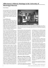
Fig. 7 Design drawing for the device described by E. Wilczynski (University of Chicago).
The drawing was produced by Wilczynski’s collaborator M. J. Eichhorn in September,
1912. See reference 16 for further operational details.
the necessity of producing such a complex
machine. With respect to this latter issue he
took the opportunity to introduce a new
design configuration for his involute of a
circle method (Fig. 8), and comments, ‘the
only apparatus required for this excessively
simple method are two protractors, preferably
of celluloid, which may be of any convenient
dimensions’. 15 Provided that the
involute arc (QR in Fig. 8) has been accurately
constructed and cut Rambaut argues
that the device should give ‘results correct
to within one or two tenths of a degree’
– that is to within about ten arc minutes.
While the precision of Rambaut’s device is
smaller than that anticipated by Wilczynski
for his machine, the cost and ease of construction
of Rambaut’s calculator provide it
with a significant utilitarian advantage
Concluding Remarks
It appears that the fate of Wren’s cycloid
method for solving Kepler’s problem was
radius OA at a position equivalent to the
orbital eccentricity (e = 0.65 in the figure).
The point E on the fixed straightedge NN
then indicates the eccentric anomaly E
(shown to be 70in the diagram). One innovative
and highly useful feature of Plummer’s
device is that in addition to determining
the eccentric anomaly it also provides a
measure of the true anomaly and the radial
distance r / a = (1 - e cos E), where a is the
semi-major axis of the orbit. Plummer only
claims that his instrument provides an approximate
solution for E, noting that highly
accurate solutions may only be obtained by
direct calculation. He does comment, however,
that given the ease with which the device
can be used, ‘[it] may be useful in preventing
any serious slip in the calculation
from being overlooked.’ 14 To this he also
adds, ‘the instrument may have some slight
educational as well as practical value’.
Rambaut’s third device for the mechanical
solution of Kepler’s problem was described
15 in the Astronomical Journal for
April 28 th , 1913. His article was written in
direct response to an earlier publication 16
on the topic written by Ernst Julius Wilczynski,
who, like T. J. J. See beforehand, was
at the University of Chicago. The device
described by Wilczynski’s not only solves
Kepler’s equation, it also evaluates the heliocentric
orbital radius r / a, where a is
the orbital semi-major axis. The device was
designed by Wilczynski and M. J. Eichhorn
circa 1912 (Fig. 7), and while never actually
constructed (as far as I can tell 17 ) the device
was developed with an eye to the ‘practical
question of cost’. The stated accuracy of the
device was such that it should have been
able to provide values for E (shown on the
Fig. 8 Rambaut’s two protractor method for solving Kepler’s equation. The solution method
is based upon the involute of a circle scheme illustrated earlier in figure 5. Image from
reference 15.
upper vernier scale) to ‘the nearest minute
of arc’. 16
Rambaut was not greatly impressed by Wilczynski’s
paper, and he begins his animadversions
by noting that Wilczynski’s claim
to novelty in the device along with its underlying
reference to ‘a forgotten theorem’
in Newton’s Principia were not new; the
method is essentially that due to Wren, and
the design is almost identical to Plummer’s
1906 calculator. Rambaut also questioned
to be one of continual re-discovery, and
the last mechanical device (that the author
is aware of) which utilized its solution
method was described 18 by Assen Dazew
in 1934. The Smithsonian Astrophysical
Observatory / NASA-run astrophysics database
system (see note 5) lists just this one
publication for Dazew, and his address is
simply given as ‘Sofia’. Dazew apparently
made a wooden prototype and then a metal
12 Bulletin of the Scientific Instrument Society No. 100 (2009)

version of his machine which was similar in
design to Plummer’s 1906 device (see Fig.
6). The estimated accuracy for the metal
version of his machine is stated as being
about 1 arc second – a truly remarkable
result. Interest in the construction of new
machines to solve Kepler’s problem seems
to have dwindled from circa 1935 onwards,
although new solution tables 19 and numerous
series approximation methods were
still published after this time. 5
Finding tractable and generally applicable
solutions to Kepler’s problem has both
stretched and exercised the ingenuity and
skill of mathematicians and astronomers
alike for the past three-hundred years. The
every-day accessibility of electronic computers
in the modern era, however, has
completely obviated the need for graphical,
series approximation and analogue devices,
and in one fell swoop, starting in the early
1980s, Kepler’s vexatious equation was
placed within the domain of easily solved
problems. In this article we have barely
skimmed the surface of the very deep literature
relating to the solution of Kepler’s
problem 1 and we have, no doubt, only
barely scratched 20 the many-layered ‘fossil
record’ relating to the analog devices created
for its evaluation.
Bibliography
Danby, M. A., Fundamentals of Celestial
Mechanics (Richmond, Virginia: Willmann-
Bell Inc., 1988).
Duffett-Smith, P., Astronomy with your Personal
Computer (Cambridge: CUP, 1985).
Heget, P., The Computation of Orbits. Cincinnati
Observatory, published privately by
the author (1948).
McCuskey, S. W., Introduction to Celestial
Mechanics (Reading, Massachusetts: Addison-Wesley
Publishing, 1963).
Newton, I., Mathematical Principles of
Natural Philosophy; translated into English
by Robert Thorp. Dawsons (London, 1969).
Smart, W. M., Celestial Mechanics (London:
Longmans, Green and Co.,1953).
Wallis, J., De cycloide et corporibus inde
gentis (Typis Academicis Lichfieldianis,
Oxon, 1659).
Young, C. A., A Text-book of General Astronomy
for Colleges and Scientific Schools
(Boston: Ginn and Co. Publishers, 1899).
Notes and References
1. See, for example, the exhaustive mathematical
treatment provided by Peter Colwell
in his book Solving Kepler’s Problem
over Three Centuries (Richmond, Virginia:
Willmann-Bell, Inc., 1993). A very brief historical
review of solution methods is given
by Ennio Badolati, ‘On the History of Kepler’s
Equation’, Vistas in Astronomy, 28
(1985), pp. 343 – 345.
2. Once the eccentric anomaly E is known
then the true anomaly, the angle measured
around the orbit from the focal point and
the line of apsides, can be determined as
well as the radial distance r(). The exact
equations need not be considered here, but
they can be found in any text on celestial
mechanics – see the bibliography. The difference
between the mean and true anomaly
is described by the, so-called, equation of
centre, and a simple mechanical device for
illustrating this variation is described in M.
Beech, ‘On Two Lost American Cometaria’,
Bulletin of the Scientific Instrument Society,
No. 94 (2007), pp. 14 – 20.
3. Some trivial solutions to equation (1) do
exist. When the orbit is a circle, for example,
e = 0 by definition, and E = M at all times.
For non-zero values of the eccentricity the
only simple solutions are at perigee, where
M = 0 = E, and at apogee, where M = =
E. In between these two specific locations
there are no analytic solutions to equation
(1), and accordingly some numerical approximation
scheme must be developed to
determine E. This being said, Flandis Markley,
of the NASA Goddard Space Flight Center,
has developed a highly accurate, noniterative,
solution to Kepler’s equation. His
method is described in the article ‘Kepler
Equation Solver’, Celestial Mechanics, 63-1
(1995), pp. 101 – 111 (1995).
4. Provided a good starting value E 0
has
been determined, then for most astronomical
applications a single iteration is all that
is required to produce a very accurate solution
to equation (1) for the provided e and
M values. Indeed, the usable solution is E =
E 0
- (M + e sinE 0
– E 0
) / (1 – e cosE 0
).
5. A comprehensive listing of 123 articles
concerning the solution of Kepler’s problem
between 1609 and 1895 has been published
in the Bulletin Astronomique de
L’observatoire de Paris, 17 (1900), pp. 37
– 47 (1900). In addition, we find that the
Smithsonian Astrophysical Observatory /
NASA ADS website (http://www.adsabs.
harvard.edu/) provides reference to 185 research
papers relating to Kepler’s problem
published between 1835 and 2008.
6. Hooke and Wren, of course, were longtime
friends and founding members of the
Royal Society of London. Hooke’s diary
accounts afford us a great insight into the
life of a man who was essentially the first
salaried (albeit poorly) scientist in England.
For diary details see, Henry W. Robinson
and Walter Adams, eds, The Diary of Robert
Hooke, 1672-1680, transcribed from
the original in the possession of the Corporation
of the City of London (London:
Wykeham Publications, (1968). For a brief
review of Hooke’s very inventive life see
Allan Chapman, ‘Experimental Astronomer’,
Astronomy Now, 17-10 (2003), pp. 68-71.
7. The cycloid has, in fact, many interesting
and diverse properties, and it has found
application in the design of load-bearing
bridge arches, the equal travel-time curve
(the so-called tautochrone), the truly isochronal
pendulum (as developed by Christian
Huygens), and remarkably it also describes
the time variation of the cosmological
scale factor in a closed Friedman model
universe.
8. C. Pritchard, ‘Two Mechanical Solutions
of Kepler’s Problem’, Monthly Notices of
the Royal Astronomical Society, 37 (1877),
pp. 354 – 358.
9. M.A. De Gasparis, ‘On Kepler’s Problem’,
Monthly Notices of the Royal Astronomical
Society, 37 (1877), pp. 263 – 265
(1877). Gasparis (1819 -1892) was Professor
of Astronomy at the Royal University of
Naples, Italy. He specialized in the search
for asteroids (discovering 9 in total) and
was awarded the Gold Medal of the Royal
Astronomical Society in 1851 for his work
in this area. He published numerous papers
on the approximate series solution of Kepler’s
equation.
10. The Radcliffe Observatory was founded
at Oxford University in 1772 and was originally
operated under the purview of the Savilian
Chair of Astronomy. In 1839, however,
the new role of Radcliffe Observer was
created to oversee observatory operations.
Rambaut was Radcliffe Observer from 1897
until the time of his death in 1923. His early
career, however, was spent at the Dunsink
Observatory in Ireland, where he worked
with Sir Robert Ball. In 1892 Rambaut succeeded
Ball as Andrews Professor of Astronomy
and Royal Astronomer of Ireland.
He moved to the Radcliffe Observatory in
1897 where he developed a programme
to study stellar proper motions and parallax
reductions in Kapteyn’s ‘selected areas’.
He also studied binary star orbits, and began
pioneering work with W. E. Wilson on
the study of solar radiation. Rambaut was
elected a Fellow of the Royal Society in
1900. Further biographical details can be
found in Rambaut’s obituary published in
the Proceedings of the Royal Society A.,
106 (1924), pp. ix – xii.
11. A. Rambaut, ‘A Simple Method of Obtaining
an Approximate Solution of Kepler’s
Equation’, Monthly Notices of the Royal
Astronomical Society, 50 (1890), pp. 301
– 302.
12. A. Rambaut, ‘A Simple Method of Obtaining
an Approximate Solution of Kepler’s
Equation’, Monthly Notices of the Royal
Astronomical Society, 66 (1906), pp. 519
– 521.
Bulletin of the Scientific Instrument Society No. 100 (2009)
13

Notice Board
Rittenhouse: Special Issue
There will be a special 80-page issue of
Rittenhouse: Journal of the American
Scientific Instrument Enterprise on ‘Science
and Early Jamestown,’ edited by Robert Hicks
and Steven Turner, and comes just after the
400th anniversary of this English settlement in
the New World. Of particular interest are the
scientific adventures of Captain John Smith,
and the analysis of recent archaeological finds
of chemical and apothecary vessels, sundials,
medical instruments, etc., but there is much
else besides. The issue is available singly for $18,
from either of the co-publishers (David Coffeen,
or Raymond V. Giordano). For subscribers to
Rittenhouse, this special issue is automatically
sent as one of the two issues of Volume 21 ($30
U.S., $35 overseas, for the volume). Volume 22
is in preparation, and will present the papers
from the SICU2 conference in Mississippi.
To subscribe or learn more about the
Rittenhouse Journal please go to the Journal’s
website: http://www.rittenhousejournal.org
Online Scientific Instrument
Trade Catalogues
With the help of Paolo Brenni, an additional
online location for ‘Online Scientific Instrument
Trade Catalogues’ has been added to the SIC
website: http://www.sic.iuhps.org/refertxt/
13. See, T. J. J. See, ‘A General Method for Facilitating
the Solution of Kepler’s Equation
by Mechanical Means’, Monthly Notices of
the Royal Astronomical Society, 55 (1895),
pp. 425 – 429.
14. H.C. Plummer, ‘Note on a Mechanical
Solution of Kepler’s Equation’, Monthly Notices
of the Royal Astronomical Society, 67
(1906), pp. 67 – 70.
15. A. Rambaut, ‘The solution of Kepler’s
Problem’, The Astronomical Journal, 27
91913), PP. 182 – 183.
16. E.J.A. Wilczynski, ‘A Forgotten Theorem
of Newton’s on Planetary Motion, and an
Instrumental Solution of Kepler’s Problem’,
The Astronomical Journal, 27 (1913), pp.
155 – 156 (1913).
17. A search through the U.S. patents database
found no registration for any device
under the names of Wilczynski or Eichhorn.
While Eichhorn’s design plan (see reference
16 and Fig. 6 here) is dated September
29 th , 1912 the idea for the device probably
dates back to at least a year earlier. This latter
supposition is based upon the title and
review of a talk given by Wilczynski at the
30 th meeting of the Chicago Section of the
American Mathematical Society held April
5 – 6 th , 1912. The summary of Wilczynski’s
talk, which had the same title as that given
in the publication listed in reference 16
(the last title word Problem, however, being
switched to Equation), describes the
possibility of constructing a mechanical device,
‘by which r (the heliocentric distance)
may be obtained without any calculation
whatever.’
18. A. Dazew, ‘Ein mechanischer weg zur losung
der Keplerschen gleichung’, Astronomische
Nachrichten, 253 (1934), pp. 191-
192.
19. See for example Glen H. Draper, ‘Tables
for the Solution of Kepler’s Problem’, Astronomical
Journal, 45 (1936), pp. 140-143.
Draper worked at the U.S. Naval Observatory
in Washingon, D.C. and this suggests
the preferred method to solve Kepler’s
equation there was via numerical tables
and interpolation techniques.
20. There are at least two other ways of
solving Kepler’s problem that have not
been described in the main text. One approach
is to construct a nomograph which
consists of three co-planar curves such that
a straight line cutting through the curves
provides the solution being sought. For
Kepler’s Problem two of the curves are
straight lines (graduated to represent the
eccentricity and mean anomaly) and the
third curve is constructed according to a
specific trigonometric equation. Thorton
C. Fry, of the University of Wisconsin, published
a detailed set of nomograph curves
for Kepler’s problem in the article, ‘Graphi-
catalogs.htm This is the ‘CNAM: List of
Catalogues of Makers / Liste des catalogues de
constructeurs’. The library of the Conservatoire
des Arts et Métiers in Paris has a series of 74
historical trade catalogues online. Most of them
are related to instrument makers.
The Scientific Instrument Commission’s
website of trade catalogues is constantly
updated and lists the most important web
addresses where it is possible to find online
scientific instrument trade catalogues.
Another website well worth a visit is http://
humboldt.edu/~scimus/LitIndex.html where
Richard Paselk, professor of chemistry and
curator of the Scientific Instrument Museum
of Humboldt State University, Arcata, California,
has listed some catalogues as well as a fair
collection of instrument manuals, including half
a dozen Leeds & Northrup manuals and some
Ainsworth balance literature.
Prestigious Paul Bunge Prize
The German Chemical Society (Gesellschaft
Deutscher Chemiker) extends an invitation
for international applications for the Paul
Bunge Prize 2010, awarded by the Hans R.
Jenemann Foundation, which is administered
by the German Chemical Society and
the German Bunsen Society for Physical
Chemistry (Deutsche Bunsen-Gesellschaft für
Physikalische Chemie).
cal Solution of the Position of a Body in an
Elliptical Orbit’, Astronomical Journal, 29
(1916), pp.141-146 (1916). The second approximation
method not discussed in the
main text is that due to Jacques Cassini.
Writing in 1719, Cassini’s method is purely
geometrical in its approach and is based
upon a series of assumptions concerning
approximately parallel lines and nearly
equal angles. The Reverend John Brinkley,
Andrews Professor of Astronomy at the
University of Dublin from 1792 to 1827
commented on the Cassini method that,
‘the facility with which this near approximation
may be obtained, renders it highly
valuable, when combined with the method
of extending at pleasure the approximation’
(see, ‘An Examination of the Various
Solutions of Kepler’s Problem and a Short
Practical Solution of that Problem Pointed
Out’, Transactions of the Royal Irish Academy,
9 (1903), pp. 83-131). In other words
the Cassini method gives a good value for
E 0
which after one or two iterations should
provide a good solution to Kepler’s equation
(see note 4). At least two mechanical
devices were constructed along the lines
dictated by the Cassini approximation.
Author’s address:
Campion College
The University of Regina, Regina
Saskatchewan, Canada S4S 0A2
e-mail: beechm@uregina.ca
The prize is endowed with 7.500 Euro and
honours outstanding publications in German,
English or French in all fields of the history
of scientific instruments. In addition to the
scientific work, applications should also include
a curriculum vitae and a list of
publications.
The deadline for nominations and selfnominations
is September 30, 2009. The
Advisory Board of the Hans R. Jenemann
Foundation will decide on the prize winner.
The prize is named after the most important
designer of analytical, assay and highperformance
precision balances in the second
half of the 19 th century, Paul Bunge. It will
be awarded in May 2010 on the occasion
of the conference of the Deutsche Bunsen-
Gesellschaft für Physikalische Chemie in
Bielefeld.
Submit your nominations to:
Gesellschaft Deutscher Chemiker
Barbara Köhler, b.koehler@gdch.de
Varrentrappstr. 40-42,
60486 Frankfurt/Main, Germany.
You may remember that the 2008 prize was
awarded to Alison Morrison-Low for her
book Making Scientific Instruments in the
Industrial Revolution (Ashgate & National
Museums of Scotland, 2007).
14 Bulletin of the Scientific Instrument Society No. 100 (2009)