Introduction to Excel Part One - MSU Educational Technology ...

Introduction to Excel: Part 1 

http://edutech.msu.edu/online/Office2007/PptXcl2007/tutorials/Excel200... 

1 of 12 10/6/2009 3:02 PM 

Introduction to Excel Part One 

Purpose 

Upon completion of this session you will be able to: 

1. 

2. 

3. 

Describe the general purposes and uses of an electronic spreadsheet 

Modify and format an existing Excel spreadsheet 

Output an excel spreadsheet to a flash drive, printer, and chart 

Software Needed 

Microsoft Excel. Please note that the screenshots are from a Windows machine, however, the 

same steps would apply to a Mac platform. 

Prerequisite Knowledge and Skills 

Before beginning this tutorial please make sure that you have completed all of the Word 

tutorials. You should have also completed all of the Basic Computing tutorials. 

Overview 

Electronic Spreadsheet 

Common elements of Spreadsheet window 

Unique elements of Spreadsheet window 

Spreadsheet cells 

[back to top] 

Lesson 1: Electronic Spreadsheet 

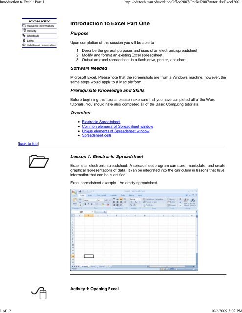
Excel is an electronic spreadsheet. A spreadsheet program can store, manipulate, and create 

graphical representations of data. It can be integrated into the curriculum in lessons that have 

information that can be quantified. 

Excel spreadsheet example - An empty spreadsheet. 

Activity 1: Opening Excel



2 of 12 10/6/2009 3:02 PM 

In this activity you will be opening the spreadsheet program Microsoft Excel and entering text 

into an Excel document. 

There may be an Excel 

icon on the desktop or in 

the status bar at the 

bottom of the screen. 

Clicking on the icon will 

launch the Excel 

program. 

1. 

Turn on your computer. 

2. Click on the Start button 

then click on All Programs> Microsoft 

Office> Microsoft Office Excel 2007. (For Macs go to the Finder Menu and click on 

Go then click on Applications. In the Application window click on the link to Microsoft 

Office. In the Microsoft Office window click Excel. ) 

Elements of importance: 

Columns 

Rows 

Cells 

We will discuss these elements further in this tutorial. 

Activity 2: Downloading, Saving and Opening an Existing File 

This activity will use a file entitled demoXP.xls that has already been created and saved on 

the Edutech site. To download and save this file: 

Link for the Excel Demo 

spreadsheet 

Right Click Here 

1. Right click here 

2. Select Save Target As... (In FireFox you will select Save Link As.) 

A Save As dialogue box will open allowing you to change the file name and the location 

where the file is saved. You should include your initials in the file name and choose a 

folder location where your course files are stored on the hard drive. In previous tutorials 

you should have created a course work folder and a CEP 810 folder. Save this file in 

your CEP 810 folder. 

3. Click on Save and the demoXP.xls spreadsheet will be saved to your folder. 

To Open the File: 

1. Click once on the Microsoft Office Button and click on Open. 

2. Navigate through your folder directory and click on the demoXP file. (You should have 

added your initials to the file name.)



3 of 12 10/6/2009 3:02 PM 


Lesson 2: Spreadsheet Window - Elements Common with Microsoft 

Word 

In this next lesson you will learn about the main elements of the Excel window. The elements 

shown below are similar to elements found in Microsoft Word. 

Title Bar 

The Title Bar lists the name of the software program you have open and then 

lists the name of the specific document you are viewing. In this case, Microsoft 

Excel is open with the document name of Book1 showing. Microsoft and other 

software use a default naming system of Book1, Book2 etc., to automatically 

name files until you change the name to a descriptive word meaningful to you. 

Because you have opened the demoXP file, your title bar should show the 

name of that document. 

Ribbon Tabs 

The terms (words) in the Ribbon Tabs each represent a different toolbar set. 

To view the set click on the word. The options in each ribbon represent 

functions that are relevant to the term on the tab. 

Ribbon 

The Ribbon has icons for frequently used items. This bar will change based on 

the tab you select.



4 of 12 10/6/2009 3:02 PM 

Scroll bar 

The Scroll Bar allows the viewer to view different parts of the spreadsheet that 

may not be viewable because of the screen size. You can move the vertical 

scroll bar up or down and the horizontal scroll bar left or right. 

Status Bar 

The left side of the Status Bar shows the possible states you have for each 

cell; Ready, Enter, or Edit. 


Lesson 3: Spreadsheet Window - Unique Elements 

These elements are unique to Excel and other electronic spreadsheets. 

Formula Bar 

The Formula Bar shows the selected cell on the left. The fx box on the 

right provides an area for entering data or formulas into the cell. 

Column & Row 

Header 

In the Column & Row Header, each column is labeled with a letter 

and each row is associated with a number. The columns, which go



5 of 12 10/6/2009 3:02 PM 

from the top of the page to the bottom, just like a column on a building, 

begin with A and go through the alphabet repeatedly with a letter 

sequence of AA, AB, ...IV until 256 columns have been identified. The 

rows are numbered from 1 - 65,536. 

Column 

Each Column can be selected by clicking on the corresponding letter on 

the spreadsheet. Numerous columns can be selected by clicking and 

dragging the cursor over the letters. 

Row 

In turn, each Row can be selected by clicking on the corresponding 

number on the spreadsheet. Numerous rows can be selected by clicking 

and dragging the cursor over the numbers. A hint: When selecting many 

rows, start from the row furthest from the beginning and drag the mouse 

upward to control the "runaway mouse". 

Cell 

A Cell is the union of a column and row. The wide black line around the 

cell means that the cell has been selected using a single left click. A 

square box (AutoFill handle) appears on the lower right edge. We will talk 

more about the AutoFill in another lesson.



6 of 12 10/6/2009 3:02 PM 

Tabs 

The Sheet Tabs are located at the bottom of the spreadsheet and serve 

as navigation tools for the workbook. A sheet is a single spreadsheet. A 

workbook (excel file) may have multiple sheets. Three sheets are 

provided when you open the workbook but more can be added by 

selecting Insert > Worksheet from the standard toolbar. The current 

worksheet will have the lighter background and extra sheets will be 

darker. To change from one worksheet to another, just click on the 

worksheet tab you want to view. Sheet names can be easily changed by 

double clicking on the text "Sheet1" and typing the new name when the 

original letters are highlighted with a black background. 

The arrows serve as navigation tools also. The vertical line with the left 

pointing arrow will take you to the leftmost sheet in the workbook. 

Correspondingly, the right pointing arrow with the horizontal line brings 

up the rightmost worksheet. The individual arrows move to the previous 

or next worksheet. 

Cursor 

The wide white Plus Symbol serves as a selecting cursor. With the 

cursor in this state, you can select a cell using a left click. The cell then 

becomes highlighted with the wide black rectangle. 

The blinking I Beam or Insertion Point is visible when the cell is in the 

Ready state and you have either double clicked into the cell or have put 

data into the cell. Even though the I Beam is common in other programs, 

the difference is that an extra action (double clicking or typing) is 

necessary for this to appear. 

Nomenclature 

The cell is named by listing the column letter first followed by the row 

number. In this example; A1 refers to the cell in the first column of the 

first row. Remember that the formula bar displays the name of the 

highlighted cell. 

Entry Bar 

There are two ways to activate the enter or edit mode of the cell. You 

can double click in the cell or single click in the Formula Box located in 

the formula bar. When you are in this enter or edit mode, additional icons



7 of 12 10/6/2009 3:02 PM 

appear next to the entry bar. The 

is used to delete content in the 

cell, the is used to accept the entry you have made and the is 

used to insert a formula. Note that the black line surrounding the cell 

becomes thinner when the cell has been activated. 

Selected Cell(s) 

The wide black line surrounding the cell or selection of cells indicates the 

Selected Cells. Any changes made in the program will occur in those 

cells. Cells need not be adjacent to one another to be selected. This will 

be covered in later lessons. 


Lesson 4: Spreadsheet Cells 

For this next lesson you will be working with the demoXP file. Please make sure you have the 

file open. You will be exploring some of the elements in an existing spreadsheet. Therefore for 

many of the steps in these activities there will be an accompanying explanation. 

Activity 1: Values and Formulas 

1. 

Single click on cell B13 (You should see the data next to fx displayed like the 

image below.) 

Remember - there are 

two levels when clicking 

in the cell - single click 

and double click



8 of 12 10/6/2009 3:02 PM 

Result: Cell B13 shows the value of 24430 but the formula bar displays the 

underlying formula of one-half of the sum of cells B4 through B12. 

Adding Values 

When keying in numbers, the keypad at the right hand side of the desktop keyboard is 

helpful. Make sure the Num Lock key has been selected. 

After entering data in the cell, you can press Enter, TAB or any arrow key to move to 

adjacent cells. This will confirm the cell's data entry. 

Edit mode allows you to edit a cell's content. There are two ways to accomplish this task. 

Double click on the cell and enter your data. 

Click on the cell and then click on the formula bar to make changes. The enter, 

cancel and function arguments will appear allowing you to accept, cancel your entry 

or add a formula from the formula bar 

To begin adding values: 

1. Click on cell C4 

2. Key in 15000. Press the Enter key or down arrow key to move to cell C5 Key in the 

remaining values in the rest of this column... (Remember to press the enter key or 

down arrow after each value has been entered.) 

5000 

0 

0 

160 

1500 

1000 

2500 

2500 

3. Click on Save in the Quick Access toolbar. Remember to periodically save your 

file.



9 of 12 10/6/2009 3:02 PM 

Activity 2: Copying and Pasting Formulas 

In this activity you will learn how to copy a formula from one cell and paste it into another. 

Remember - if you single 

click on a cell to change 

data, you may overwrite 

current data by mistake 

- always double click on 

the cell or use the 

formula bar. 

1. Click on cell B13 

2. On the Home tab, select Copy (You should see a dotted line (marquee) around cell 

B13.) 

3. Click on cell C13 

4. On the Home tab, select Paste 

5. Press Enter or Esc to stop the copying of subsequent cells (You will no longer see 

the dotted line around cell B13.) The number 13830 should appear in cell C13. 

Notice the marquee around cell B13 reminding you that the content of this cell has 

been copied. 

Activity 3: Entering Formulas 

In this activity you will enter a formula that will add the columns B4 and C4 

1. 

2. 

Double click on cell D4 and type =sum(b4:c4) 

Press Enter to confirm the entry 

The formula box for the 

row and column labels is 

not case sensitive so 

typing b4 will result in B4 

in the cell. 

Note: Using the sum function is more flexible than simply adding the two columns together 

since the sum function will allow you to easily add additional columns if you were to include 

a Phase 3 to the formula. 

Example: [=(B13+C13+D13)] vs. [=SUM(B13:D13)] 

When using the sum formula, the colon (:) is used to select the adjacent cell and the comma 

(,) is used to select non-adjacent cells. This formula [=SUM(B4:C4,B6:C6)] would give the



10 of 12 10/6/2009 3:02 PM 

sum of the adjacent cells, B4 & C4 added to the sum of adjacent cells B6 & C6. 

Result: The value displayed in the cell D4 should be 30000 with the cursor in a ready 

position in cell D5. 

Activity 4: Copying Formulas into Multiple Locations 

In this activity you will learn how to copy and paste a formula into multiple cell locations. 

You will copy and paste the formula from D4 into cells D5 through D13. 

1. 

2. 

Select cells D4 through D13 by either clicking on D4 and dragging down to D13 or 

clicking on D4 and holding down the Shift key and then clicking on D13. 

On the Home tab, select the Fill Down button. 

Result: The formula and values should be displayed in cells D5 through D13. Cell 

D13 should display the number 38260. 

Additional Information: Fill Down can be used with adjacent cells and does not require the 

use of the clipboard which uses copy and paste. The Fill Down action provides a Relative 

Reference to the cells. This means that the formula will remain the same but the cell letters 

and numbers will reflect the currently selected rows and columns. If you want to learn more 

about Relative vs. Absolute Reference in cells, check the help menu. 

Alternate Method: An alternate way to complete the Fill Down is to select the cell to be 

copied, then click and hold the small black box or handle on the edge of the cell, then drag 

until you have selected all of the cells you want filled.



11 of 12 10/6/2009 3:02 PM 

Activity 5: Entering Additional Formulas 

In this activity you will learn how to add additional formulas to the spreadsheet. You will 

enter a sum formula to total Phase 1, Phase 2, and the Grand Total. 

1. 

2. 

Click on B14 and enter =sum( 

Drag from B4 through B13 and key in a right parenthesis and press Enter 

Result: The value of 73290 should be displayed in cell B14. 

Alternate Method: An alternate way to include the Sum formula is to click on cell B14 and 

then click on the Sigma symbol for summation and select and drag through B4 through B13.



12 of 12 10/6/2009 3:02 PM 

Now you are ready to add the totals for Phase 2 and the Grand Total. 

1. 

2. 

Copy and paste the formula from B14 into C14. Remember to click Enter or Esc to 

stop copying. 

In cell C14, enter the formula to sum column D 

The spreadsheet calculations are complete. 

Wrap Up: 

Go Back to Tutorials 

http://edutech.msu.edu/online/ 

Evolution of the Spreadsheet: 

The first electronic spreadsheet, known as VisiCalc, was developed by Dan Bricklin and Bob 

Frankston. While an MBA student at Harvard, Dan used this spreadsheet concept to crunch 

numbers in a case study around Pepsi-Cola's marketing campaigns. This software soon 

became one of two "killer apps", (along with word processing) that influenced personal 

computer growth. Today the electronic spreadsheet is used in numerous fields for asking 

"what if" questions and providing immediate answers by using formulas to perform 

calculations. To read more about the development of electronic spreadsheets, visit Dan 

Bricklin's Web site www.bricklin.com. 

Workbook: 

As spreadsheets became larger, they became more difficult to manage. The concept of a 

workbook was developed to manage this collection of spreadsheets. In this lesson, you have 

opened a sheet within a workbook in Excel. The default number of sheets included in a 

workbook is three but you can add as many sheets as needed depending on the memory 

available on your computer. For more advanced tips, check out the tutorial web site created 

by School of Information, University of Texas at Austin. 

In the next section, Excel Part 2, we will begin with lessons on how to format a spreadsheet.


http://edutech.msu.edu/online/Office2007/PptXcl2007/tutorials/Excel2007-02.html 

Page 1 of 11 

10/15/2007 

Introduction to Excel Part Two: Formatting an Existing 

Spreadsheet 

Purpose 

Upon completion of this tutorial you will have learned how to format the following: 

• Labels 

• Title 

• Rows and columns 

• Values 

• AutoFit Selection 


Microsoft Office Excel 


Before beginning this tutorial please make sure that you have completed Excel Introduction - 

Part 1. 

Overview 


• Formatting 

• Creating a Chart 

Lesson 1: Formatting 

All of the activities in this lesson will focus on formatting the spreadsheet. In this lesson you 

will learn how to format labels, titles, and values. You will also use functions like AutoFit that 

will automatically format the width of columns or rows. 

Activity 1: Spreadsheet Labels 

Purpose: To improve the appearance and readability of the spreadsheet 

1. Select Row 3 by clicking on the row header. Remember that the row header is 

the number at the beginning of the row. 

2. Click on the Bold button 

3. Click on the Centering icon 

Remember to save your 

file often. Click on the 

Save icon, press Ctrl S, 

or use the File menu to 

select Save. 

Result: Column titles are bold and centered 

1. Select Column A by clicking in the column header 

2. Click on the Bold button



Page 2 of 11 

10/15/2007 

3. Click on the Align Right button 

Result: Categories are bold and right aligned 

Activity 2: Spreadsheet Title 

The Merge and Center 

icon is a toggle button 

so it can be turned on 

and off. 

1. Select the title cell - B1 

2. Click on the arrow in the Font Size box, select 16 (See image below) 

3. Click on the Bold button 

4. Select cells A1 through D1 

5. Click on the Merge and Center icon



Page 3 of 11 

10/15/2007 

Result: Title is reformatted 

Activity 3: Formatting Values 

Purpose: To make values easier to read 

1. Select the box of cells -- B4 through D15 

2. Click the icon under the Number section of the Home tab 

3. Click on Accounting from the Category menu. Then on the right side of the 

Format Cells window make sure that Decimal Places is set to 2 and Symbol is 

set to None 

4. Click on OK



Page 4 of 11 

10/15/2007 

Result: All values are formatted with commas and two decimal figures 

5. Select cell D15 

6. On the Home tab, select the Currency button 

7. Set Symbol to $



Page 5 of 11 

10/15/2007 

Result: Grand Total is formatted with a dollar sign 

Activity 4: AutoFit Columns 

1. Select the entire worksheet by clicking the Select All Button in the upper 

left corner where the rows and columns intersect. 

2. Select the Format button (from the Home tab on the ribbon) and then AutoFit 

Column Width 

Result: All of the columns are spaced to accommodate the widest content in each



Page 6 of 11 

10/15/2007 

column. 

Make sure you save your file. 

Activity 5: Page Set Up 

Purpose: To format the spreadsheet for printing 

1. In the Ribbon menu, choose the tab and select the icon in the 

Page Setup area 

2. Click on the Page tab, make sure the Orientation is set at Portrait 

3. Select the Margins tab and under the section Center on Page, check the box 

next to Horizontally 

4. Select the Sheet tab and under Print, check Gridlines (this will add lines to the 

worksheet when printed) 

5. Then press OK 

6. In the File menu choose Print Preview... to see the placement of your worksheet 

on the page. 

7. Save your Excel Document. 


Lesson 2: Creating a Chart 

Excel is not only used to perform computations or to sort and organize data. It can also be 

used to create graphical representations of information.



Page 7 of 11 

10/15/2007 

Activity 1: Creating a Chart 

Purpose: To produce a graphic display of project budget totals 

*Non-adjacent cells will be selected to create this chart. 

Placing the date in a 

Header or Footer is 

helpful on a 

spreadsheet because of 

the many times the data 

is changed and printed. 

Also, placing the chart 

name in the Header is 

helpful when there are 

numerous pages in a 

spreadsheet. 

1. Select cells A4 through A13 

2. With the previous cells selected, hold down the Ctrl key, click and drag from D4 

through D13 

3. Click on the Column icon on the tab 

5. Select a 3-D Clustered Column from the Chart Type menu



Page 8 of 11 

10/15/2007 

6. A new chart is created and appears in the middle of your worksheet. Also, the Chart 

Tools tabs appear on the ribbon (there are three tabs) 

7. Select the Move Chart button from the Design tab in the Chart Tools area of the 

Ribbon. (Click once on the chart if the Chart Tools are not visible.)



Page 9 of 11 

10/15/2007 

8. In the Move Chart dilogue box select New sheet, name the sheet "Totals Chart" 

and click OK 

9. The chart is now on its own worksheet in the workbook. Note the tab named 

"Totals Chart" at the botom of the window 

Notice: The chart worksheet tab includes the name Totals Chart that you provided 

while using the chart wizard. Sheet 1 corresponds to the data we have in the 

spreadsheet. 

10. Select the Layout tab, click the Legend button, and select None 

11. Double click on the Sheet1 tab that is adjacent to the Totals Chart tab. 

12. Rename your data sheet to Budget Data. 

13. To change the orientation of the text for the Budget Categories, click on one of the 

labels and choose the Format tab. Click the format selection button.



Page 10 of 11 

10/15/2007 

14. A Format Axis dialogue box appears. Select Alignment from the list on the left 

and choose Rotate all text 270º from Text direction 

15. Click the Microsoft Office button and select Print > Print Preview 

16. If the chart appears the way you want it to look when printed, click on Print 

17. If you would like to make changes to the appearance or add a Header or Footer, 

click on Setup and select the options you would like to change.



Page 11 of 11 

10/15/2007 

Result: Chart with viewable text representing each category 

Wrap Up: 

You have just completed the Introduction to Excel - Part II which included: 



1. General purposes of electronic spreadsheets 

2. Modify and format an existing Excel spreadsheet 

3. Output an excel spreadsheet to a flash drive, printer, and chart 

In the next section, you will create your own spreadsheet and learn many fascinating ways to 

manipulate data to help with student understanding of various concepts.

Introduction to Excel- Part 3 


Page 1 of 18 

10/15/2007 

Introduction to Excel Part Three: Creating a New 

Spreadsheet & Performing Data Computations 

Purpose 

Part 3 is a continuation of an introduction to Excel. In this tutorial you will learn how to: 

1. Open a new file 

2. Enter column labels & data 

3. Format data 

4. Compute data using a formula 

5. Sort data 

6. Create a header for a spreadsheet 

7. Filter data 

8. Create a custom filter with a single criterion 

9. Create a custom filter with multiple criteria 

10. Subtotal data 

11. Create a chart with subtotals 


Microsoft Excel 


Before beginning this tutorial please make sure that you have completed Excel Introduction - 

Parts 1 & 2. 

Overview 

Excel is a spreadsheet that has many functions, one of which is the ability to ask questions of 

or query the data that is presented. In these lessons you will have the opportunity take a 

blank workbook and turn it into a vehicle for exploring information by sorting and filtering data 

according to specific criteria or characteristics. This formatted and queried data can then be 

subtotaled, and charted allowing further comparison and contrast of data. 

When these lessons have been completed, you should have the basic knowledge, comfort 

level, and skill set for using a spreadsheet for your own classroom subject matter application. 


• Creating a New Spreadsheet 

• Data Computations 

Lesson 1: Creating a New Spreadsheet 

In the previous lessons, the spreadsheet was started for you. In this lesson you will start with 

a blank spreadsheet and enter, format and manipulate data to allow for more thoughtful, indepth 

interpretation of the raw data. 

Activity 1: Open New File 

1. From the Microsoft Office Button, choose New 

2. With the Blank Workbook selected, click on Create 

Result: Blank Spreadsheet 

Activity 2: Entering Column Labels & Data



Page 2 of 18 

10/15/2007 

1. Key in the following labels in Row 1 

Country 

Continent 

Population 

Total Area 

Life Exp 

Pop Growth 

Here's a shortcut...An 

easy way to view data 

from two sources, is by 

minimizing both 

screens, placing them 

beside one another and, 

re-sizing them so there 

is no overlapping of the 

documents. You can 

move easily from one 

document to the other 

with no lengthy reloading 

of each 

document screen. 

2. Starting with Row 2, key in the following: 

United States 

North America 

298444215 

9631420 

77.85 

.0091 (The data given .91 is in % format so we will need to enter the raw 

data and format the cells to have the correct data for calculations) 

3. Press Enter and then the Home key to start at cell A3 

Data for this spreadsheet is available at The World Factbook Web site... 

https://www.cia.gov/cia/publications/factbook/ 

Just select the country in the pull down menu. 

4. In Row 3, key in the following 

France 

Europe 

60876136 

547030 

79.73 

.0035 

5. Since some of the data may not be visible due to the default column width 

it may appear as a series of pound symbols (##########). Use the 

AutoFit Column Width option under the Format button to automatically 

re-size the column widths. Remember to first use the Select All Button to 

make sure all data is included. 

6. Save Sheet 1 as Countries. Remember to double click on the sheet tab 

and type in Countries.



Page 3 of 18 

10/15/2007 

7. Using the CIA Web site provided, fill in the data on the following countries 

(Remember to use the drop down menu to go to the country page and then 

scroll down for the data): 

Argentina 

China 

Chad 

Denmark 

Egypt 

Chile 

Japan 

Canada 

Algeria 

• An alternate way to fill in the spreadsheet is to use the Data Form. A 

single record is visible, allowing for ease in entering the data. 

• To use the Data Form, you must add the button to the Quick Access 

menu. 

• Click the drop-down arrow on the right side of the Quick Access menu



Page 4 of 18 

10/15/2007 

and choose More Commands. 

• In the Excel Options window select Customize from the menu on the left 

and click the drop-down menu under the Choose commands from option 

• Select Commands Not in the Ribbon 

• Scroll through the list to find the Form button, click it once, and click the 

Add button



Page 5 of 18 

10/15/2007 

• The Form button now appears as part of the Quick Access menu 

• Highlight the data, in cells A1 through F13. In the Quick Access menu, 

select the Form button 

• This box appears with the header row as the field names. 

• The first record is visible in the individual field locations. The current record 

being viewed along with the total number of records is provided. You can 

select Find Next to go to the next record, Find Prev to take you back a 

record, Delete the current record, add a New blank record, search using 

specific Criteria, or Close the form. 

• Make yourself familiar with this form and then add the remaining countries. 

Pressing Enter is another method of taking you to a new empty field. Tab 

will take you to the next field in the record. Select Close when finished. 

Activity 3: Formatting the Data



Page 6 of 18 

10/15/2007 

Remember that text by 

default is center justified 

and numbers are right 

justified. 

1. Format the population and total area data as accounting with 0 decimal 

places. Remember to highlight the data first, then apply the formatting. 

2. Format Life Exp data as numbers with 2 decimal places. 

3. If an individual column does not properly display the data, (remember the series 

of pound symbols (##########)), another way to re-size the column is by 

mousing over the right edge of the column until the double sided arrow 

appears. Double click and the individual column will adjust the width to fit the 

data. 

4. Format Population Growth as % with the decimal set at 2 . 

Your spreadsheet should look like this... 

Freeze pane is a helpful 

viewing tool when you 

have data that goes 

beyond the viewing area 

of your screen. The row 

and column headers 

remain in place and the 

data inside is allowed to 

move so you know the 

field and record you are 

viewing. To use this tool, 

select the View tab. 

Click the Freeze Panes 

button and select 

Freeze Panes. To 

remove this feature, 

select Unfreeze Panes. 


Lesson 2: Data Computations 

In this lesson, the country data will be computed, sorted, filtered various ways, subtotaled, 

and charted to better understand, interpret, and draw conclusions about the raw data 

presented for each country. 

Activity 1: Computing Data Using a Formula 

Now that the data is entered into the spreadsheet, you can use it to make inquiries



Page 7 of 18 

10/15/2007 

about the information on the countries by placing formulas in various cells. 

When you copy the 

formula by highlighting 

the cells and dragging 

the fill down box, you 

are using a Relative 

Reference. The 

formulas are created 

relative to or in 

relationship to the rows 

you are selecting. 

Another method of 

referencing cells would 

to use an Absolute 

Reference which 

accesses data in a 

specific cell. The 

formula would include a 

$ in front of each column 

letter and each row 

number such as 

=$A$13. 

1. Add one more column by placing the title Pop. Density in cell G1. 

2. In cell G2, enter the formula to compute the density. The formula you should 

type in the formula box is =C2/D2. The result should be 30.98652. 

3. Copy the formula into the rest of column G (cells G3-G12) by highlighting 

cell G1 and dragging the fill down box (black) in the right hand corner 

down until cells all data cells are highlighted. 

4. Format the column so the numbers show two decimal places and the field 

name is completely visible. 

Result: Data that is easily comparable to like items 

Activity 2: Sorting Data 

1. Single Click on a cell within the data set you want to sort. 

2. On the Data tab, select Sort... 

If you see the message below, you need to select any cell containing information that is 

part of this list of data. You need to tell the software which list of information you intend to 

sort. 

Another error message you may see would be the Sort Warning box if you select only a 

few cells but not all of them within your data set. Select Expand the selection button to 

include the full data set, not just the few cells that were selected.



Page 8 of 18 

10/15/2007 

3. Notice that the range of cells to be sorted is highlighted. 

4. At the top of the Sort dialogue box, make sure My Data Range has Headers is 

selected . 

5. In the Sort By section, select Continent. 

6. Click the Add Level button and in the Then By section, select Population. 

7. It is fine to leave the default order of Ascending . 

8. Click on OK. 

Result: Data sorted by Continent. Within each Continent the data is sorted by 

Population



Page 9 of 18 

10/15/2007 

Activity 3: Creating a Header for the Spreadsheet 

1. Click the Insert tab 

2. Select the Header/Footer button 

3. In the Center section type Countries Sorted by Continent 

4. Click in an empty cell to exit the Header and Footer mode 

5. Double Click on the tab for Sheet 1 and change the name to Sort by 

Continent 

Result: Sheet of sorted countries ready for printing 

Activity 4: Filtering Data 

Once the data is sorted you can use the filter command on specific records dependent 

on criteria. The records that are extracted will depend on the criteria you select. 

1. On the Data tab, choose Filter 

A series of Pop-down menu icons appear next to each field name in the header row. 

2. Click on the pop-down icon for Continent, select (Select All), and select 

Africa 

Result: Only Countries from the Continent of Africa appear (records 2, 3, & 4). 

Notice that rows 5-12 were not visible since these were filtered out from view.



Page 10 of 18 

10/15/2007 

3. To Copy this filtered data to another sheet to preserve the original data, use the 

Select All button in the corner and Copy the data. 

4. Click on the Sheet2 tab and Paste the data into the sheet. The default cell 

selection is A1 so a paste command will work. Rename the sheet tab " Filter 

by Continent". 

5. Notice the pop-down icons are no longer present and the row numbers are 

back to consecutive numbering. Only the data has been copied, not the filtering 

command prompts. 

6. The Header/Footer content does not carry over from one sheet to the next so 

you will need to repeat the commands to add a Custom Header for Filter by 

Continent of Africa. To return to these directions, click here. 

Clear Filter - All Fields 

1. Return to the original sheet that is now labeled Sort by Continent 

2. Clear the Filter command by clicking the Filter button on the Data tab 

Result: All data is displayed 

Activity 5: Custom Filter - Single Criterion 

By creating a custom filter you can specify data ranges within a column. 

To filter continents that have America as part of their name, you will use the "wild 

card" symbol of asterisk (*) in the filter criteria. The asterisk represents any series of 

characters that may be part of the filter criteria. 

1. With the filter icons still in place, Click on the drop-down icon for Continent 

2. Select Text Filters > Equals 

3. Under the heading Show row where: Continent, if the term equals is not 

already displayed, then use the drop-down menu to select equals. 

4. In the adjacent box, key in *America 

5. Press OK to complete the filter



Page 11 of 18 

10/15/2007 

Result: Countries in North and South America are displayed 

7. Copy this filtered data onto a new sheet, rename the sheet, and add a 

Header to the sheet 

Activity 6: Custom Filter - Multiple Criteria 

This section uses Boolean logic to combine terms. The words used to qualify the data 

are called operators. In reference to filtering within a column we will be talking about 

the Boolean operators and and or. 

With this data set, countries with similar size can be compared in terms of population, 

life expectancy, population growth and population density. Filtering countries with a 

total land area of more than 756,950 and less than 9,596,960 will give us this data set 

for comparison and further manipulation. 

1. Return to the Sort by Continent worksheet and Clear the Filter using the 

same method as before 

2. Click on the drop-down icon for Total Area 

3. Select Number Filters > Greater Than... 

4. Under the heading, Show row where: Total Area, use the drop-down menu to 

select is greater than 

5. In the adjacent drop-down menu, select 756,950 

6. Make sure the radio button for And is selected 

7. In the next set of drop-down menus, select is less than and then 9,596,960 

as the criteria 

8. Press OK to complete the filter



Page 12 of 18 

10/15/2007 

Notice that the filter icon arrow of the column where a filter has been applied has 

changed. 

Result: Only Countries with a Total Land Area greater than 756,950 and less than 

9,596,960 are displayed. 

Now additional comparisons can be made about the population density in relationship 

to life expectancy, and population growth for countries with similar land area. 

9. Copy this filtered data onto a new sheet, rename the sheet, and add a Header to 

the renamed sheet. A Workbook has a default of three Sheets. To add more, in 

the Insert menu, select Worksheet. A new Sheet appears on the Sheet Tab list 

to the left of the current worksheet. If you want to move this sheet to the 

rightmost position, just left click on the tab until you see the sheet icon appear. 

(It looks like the New document icon.) Drag the sheet name to the preferred 

location on the bar. An insertion arrow will appear to designate the new location. 

Release the mouse if the location is correct. 

Result: Sheet Tab is listed in user defined order 

Remove Filter - this command will remove the Filter drop-down menus from each 

column. This command is executed when you deselect Filter.



Page 13 of 18 

10/15/2007 

1. Return to the original sheet that is now labeled Sort by Continent. 

2. Go to the Data tab. Click on Filter. This command acts like a toggle switch (on 

or off). By clicking on Filter you have turned the command off. 

Result: All data is visible and Filter icons have been removed 

Activity 7: Subtotaling Data 

While the Average function can work well to average data, you may want to average 

the data according to a specified field or category and view or hide varying amounts of 

data according to that category. The Subtotal command will compute this function 

within the data set. 

1. Make sure you are in the Worksheet labeled Sort by Continent because we 

will begin with data sorted by continent. Not all of the subtotal formatting holds 

when copied, so a new sheet should be selected first. Select All (button in lefthand 

corner) and copy the data from the sheet into a new Worksheet 

2. Format your new sheet 

a. Label the sheet tab Subtotals 

b. Re-size the fields 

c. Add a header 

d. Move the Subtotal tab to the last position (far right). 

3. Click on a cell with data. Go to the Data tab and click the Subtotal button. 

4. Under the header At Each Change in: use the drop-down menu to select 

Continent. 

5. Under the header Use Function:, use the drop-down menu to select 

Average. 

6. Under the header Add Subtotal to:, click on Life Exp to check it. If any other 

box has a check mark, then click on the box to de-select it. 

7. Click on OK.



Page 14 of 18 

10/15/2007 

Result: Life Expectancy for each continent is averaged and displayed below the 

continent 

With Subtotaling, a display appears on the left side of the worksheet which acts like the 

outline feature in Word. The + and - symbols will expand or collapse (toggle) the rows 

according to the level you select. Currently all of the data is visible along with the new 

Life Expectancy averages for each continent. When all data is visible, you will see 

Level 3, represented by dots. Level 2 can collapse the rows according to the 

subtotaling criteria; in this case it is countries. Level 1 can collapse all rows with only 

the field titles appearing and the Grand Average (average of all continents) displayed. 

You can also select the numbers at the top to collapse or expand all records at that 

level. The remaining activities will allow you to further explore the subtotaling feature. 

Hiding the Detail



Page 15 of 18 

10/15/2007 

1. Click on the small number 2 in the outline report on the top left of the page. 

Result: Subtotals of Life Expectancy for each continent are displayed along with 

the Grand Average 

Activity 8: Creating a Chart with Subtotals 

The Horizontal Cylinder 

chart was chosen to 

better accommodate the 

lengthy data titles. 

Choosing different chart 

types and sub-types 

help to display the data 

in a manner that 

supports better 

comprehension. 

In this activity you are going to create a bar chart that displays all of the Life 

Expectancy subtotals for each continent. Only the data that is visible will be included in 

the chart, not data from the hidden cells and rows. 

1. Highlight cells B1-B17, press Ctrl (to include the next set of cells) then select 

cells E1-E17 

2. Click on the Insert tab and select the Bar button to create a chart 

3. Choose Cylinder



Page 16 of 18 

10/15/2007 

4. Click on the Layout tab. Click the Legend button and select None to remove 

the legend (See image below) 

Try formatting the 

various parts of the 

chart to fit your own 

style and to better 

represent the data. Click 

on the data you want to 

change, then right click 

and select Format to 

bring up a dialogue box 

with options



Page 17 of 18 

10/15/2007 

5. On the Layout tab click the Chart Title button and select Above Chart. 

6. Title the chart Life Expectancy 

Result: A Chart of Life Expectancy subtotals for each continent. 

Notice in the image above that the cells with chart data and text have a colored 

outline. The colored outline corresponds to the data and text from the spreadsheet; 

purple highlights the Continents displayed, blue highlights the data used (subtotals) for 

life expectancy and green highlights the data series title. Also notice the formula bar 

with the chart series that references the absolute values of the subtotal cells. (the ! in 

the formula refers to the worksheet named Subtotal) 

Copy Sheet 

There is a difference between copying a sheet and copying the data within a sheet. As 

you saw earlier, copying the data does not retain all of the filtering or subtotaling 

features of the worksheet. A way to allow these features is by copying the worksheet. 

1. Select Edit, then Move or Copy Sheet 

2. A new sheet with the subtotal features is created with the name of Subtotal (2).



Page 18 of 18 

10/15/2007 

Change the name of the sheet tab to Subtotal Detail and move the 

worksheet to the right of the Subtotal worksheet. 

Show Detail 

1. Click on the plus sign next to the Africa Average 

Result: The individual fields from the African countries are displayed with only 

the averages from the other continents displayed 

Notice that the chart also changed to include all Life Expectancy for countries in Africa 

because it was referencing a specific cell range. Click on the chart and using the 

keyboard select Delete since it is no longer referencing the data initially specified. 

Removing Subtotals 

1. On the Data tab, select the Subtotals button 

2. Click on Remove All 

Result: All data with no summaries displayed 

This is not a toggle button. The chart data will change and all subtotals will need to be 

re-selected if removed. 

Wrap Up: 



Excel is used to explore and answer questions by way of computing data, sorting, filtering, 

and subtotaling various data sets. You should now be able to alter this data set or create a 

new spreadsheet for use in your own educational setting with specific learning objectives 

relevant to your subject area. You will need these skills to complete the Excel assignment for 

this class. Remember that Excel is a very powerful software tool that has great potential for 

displaying and analyzing facts and figures.

Introduction to Excel Part One - MSU Educational Technology ...

You also want an ePaper? Increase the reach of your titles

Delete template?

Save as template?