Integral (Macroscopic) Balance Equations

CBE 6333, R. Levicky 1
Integral (Macroscopic) Balance Equations
The Basic Laws. A body (here, of a fluid) consisting of a given set of fluid particles with a total mass
m, total momentum p, and total energy E (E = internal + kinetic + potential) obeys the basic balance
laws familiar from physics:
1). conservation of mass m (mass balance): dm/dt = 0
2). Newton's 2nd law of motion (momentum balance): F = ma/g c = m/g c dv/dt = 1/g c dp/dt
3). conservation of energy (energy balance): dE/dt = dQ/dt - dW/dt.
dQ/dt is the rate of heat flowing into the body from the surroundings, while dW/dt is the rate at which
work is done by the body on the surroundings.
These three "laws of nature" underlie the basic postulates of transport phenomena. When expressed in
mathematical form, these laws lead to equations that can be used to solve for quantities of interest such
as velocities, flow rates, and temperature or energy changes. It is important to emphasize that the laws
1) to 3) as written are for a body through the surface of which there is no fluid flow (i.e. no
convection); thus, for all times, the body consists of the same set of particles.
The Concept of a Control Volume. It is often more convenient to solve the balance laws if they are
expressed for an open control volume through which a fluid is flowing, rather than for a closed body as
done above. Such a control volume is referred to as "fixed" if it does not change position or move in
any way with respect to the chosen reference frame. Physically, the control volume could be defined as,
for example, the contents of a reactor or some other process unit or simply as a region of space inside a
fluid phase. The next task is to express mass, momentum and energy balance laws for a fixed, open
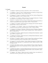
control volume (see Figure 1).
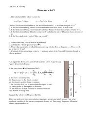
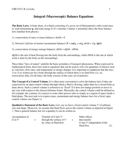
Qualitative Statement of the Basic Laws. Let's say we have a fixed control volume V' of arbitrary
size and shape. Moreover, we assume that fluid flows across the control volume as depicted in Figure
1. Then a general balance law for a quantity G can be written as:
Accumulation of Transfer of G into V' Other effects
G in V' = through the surface of V' + that transfer
by virtue of fluid flow
G into V' independent of the
fluid flow (1)

CBE 6333, R. Levicky 2
Fluid
Flow
x 3
x 2
x 1
Fig. 1
V'
Here, G is one of the three quantities of interest: total mass, momentum, or energy. Let's rephrase
equation (1) to reflect these selections of G.
If G is total mass, then:
Accumulation of transfer of mass into V' by fluid
mass in V' = flow across the surface of V' + 0 (no other effects) (2)
The external effects for mass transfer are zero because mass can only be transferred by virtue of the
fluid flow. When something is transferred by virtue of fluid flow, we say that it is transferred by
"convection." If no fluid flow occurs across the surface of V' (i.e. if there is no convection), then no
mass is transferred into V'.
If G is momentum, then (G is bold since momentum is a vector)
Accumulation of transfer of momentum transfer (generation) of
momentum in V' = into V' by fluid flow + momentum in V' due to forces
across the surface of V' acting on V' (3)
Momentum is transferred by convection (1st term on right) because the fluid that enters V' brings
momentum with it. For example, if a 1 kg piece of fluid moving at a velocity of 2 δ x m/s enters V', then
2 δ x kg m/s of momentum was brought into V' since the momentum p of the piece of fluid is p = mv =
2 δ x kg m/s. The basis vector δ x indicates that the momentum brought into V' is along the direction of
the x axis. The second term on the right of equation (3) is present because forces acting on the volume
V' will impart momentum to the fluid contained in V' according to Newton's 2nd law, F = 1/g c dp/dt.
The force term will be discussed in greater detail below.
If G is energy, then
Accumulation of transfer of energy transfer of energy into
energy in V' = into V' by fluid flow + V' by heat transfer and by work (4)
across the surface of V'

CBE 6333, R. Levicky 3
Energy is transferred by convection (1st term on right) because the fluid that enters V' brings energy
with it. Due to its nonzero velocity, the fluid possesses kinetic energy. Due to its position in a
gravitational field (and / or other potential fields, such as electric or magnetic), the fluid possesses
potential energy. Due to the molecular bond vibration, rotation, translation, etc. of the fluid molecules,
the fluid possesses internal energy. The fluid that enters V' brings the kinetic, potential, and internal
energy it has with it, and this is the source of the convective term in equation (4). The second term on
the right of equation (4) is present because transfer of heat into V' and the performance of work by the
external fluid on the fluid inside V' also result in a transfer of energy. For example, even in the absence
of convection (first term on right equals zero), heat can flow into V' by conduction or radiation. Work
can be performed on the fluid in V' by various means. For example, some type of machinery, such as a
rotating impeller, could exert force on the fluid inside V', resulting in a displacement of the fluid. The
product of this force times the displacement leads to shaft work. Another example of work performed
on the fluid inside a control volume is flow work, which represents work done by normal stresses as
they push fluid through the surface of V'. We will need to account for all such modes of energy
transport.
The statements above are qualitative, and the discussion needs to be put into a mathematical
terminology to be useful for calculations. How do we formulate the mathematical equations First, an
expression for the accumulation term on the left hand side of equations (1) - (4) will be derived.
Mathematical Statement of the Basic Laws. We will denote the amount of G per volume as g'. Thus
if G refers to mass of fluid, then g' is the fluid density (mass/volume) ρ. If G is momentum, then g' =
mv/volume = ρv (G and g' are bold faced when we associate them with momentum since momentum is
a vector quantity). If G is energy E, then g' = ρe where e is energy per unit mass of fluid; hence, ρe is
energy per unit volume of fluid.
In an infinitesimal volume dV', there is an amount of G equal to g' dV' (ex. if g' = ρ, then the volume
dV' will contain a mass of fluid equal to ρ dV'). The total amount of the quantity G in V' is then
obtained by integration (i.e. summation) over the entire volume V',
G = ∫∫∫ g' d V '
(5)
V '
The derivative of this integral with respect to time,
[ ]
dG dt = d ∫∫∫ g' dV ' dt
V '
(6)
is the rate of accumulation of G in V'. For example, the rate of accumulation of mass in V' is given by
[ ∫∫∫ ρ V ' ] t and the rate of accumulation of momentum in V' is [ ∫∫∫ ρ v V ' ]
d d d
d d dt
. Note that the
V '
V '
momentum term is actually three terms, one for each component of the momentum:

CBE 6333, R. Levicky 4
x-component: y-component: z-component:
[ ∫∫∫ ρ v x V ' ] t d[ ∫∫∫ ρ v ydV ' ] dt
[ z ' ]
d d d
V '
V '
d ∫∫∫ ρ v dV dt
(7)
V '
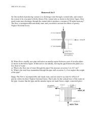
Next, an expression for the rate of convection term will be derived. The convective term is the
first term on the right hand side in equations (1) - (4). We will argue that the rate at which G is carried
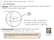
by fluid flow across a differential area dA on the surface that defines V' is equal to - g'v • n dA, where v
is the fluid velocity and n is a unit normal to the surface. Let's dissect this expression to understand it
better. - v • n is the projection of v onto the normal direction (the n direction) to the surface, and equals
the speed of the fluid perpendicular to the surface (Figure 2); the minus sign ensures that the speed is
positive when fluid flows from outside of V' into V'. It is customary to regard fluid inflow as positive
since it contributes to accumulation in the control volume, while fluid outflow is regarded as negative.
Fluid
Flow
n
surface
length of segment = -v ⋅ n
v
Fig. 2
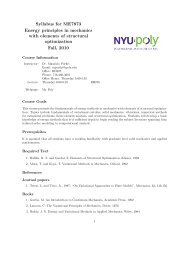
When - v • n is multiplied by dA the result, - v • n dA, equals the rate at which fluid volume flows
across dA (see figure 3); that is, - v • n dA is the volumetric flowrate into V' through the area dA (in
units of volume/time). Multiplication of the volumetric flowrate - v • n dA by g' gives the convective
inflow of G into V' through dA. Since g' is G per volume (units: G / volume), multiplying g' by the rate
at which fluid volume flows into V' (units: volume/time) equals the rate at which G is convected into V'
(units: G / time) through dA. To arrive at the total convective influx of G into V', all of the differential
contributions - g' v • n dA are summed over the entire surface of V'
∫∫ g
Rate of convection of G into V’ = − '( v ⋅ n)
d A
(8)
A

CBE 6333, R. Levicky 5
dA
n
surface
-v ⋅ n
v
Volume of fluid passing
through d A per unit time
Fig. 3
We are now ready to restate equations (2)-(4) in more mathematical terms.
1). Conservation of Mass (Mass Balance). The rate of accumulation term (equation (6)) and the rate
of convection term (equation (8)) are the only terms needed in the mass balance equation (2). G now
represents the total mass of fluid in V', and g' becomes the fluid density ρ. Thus, equation (2) is
rewritten as
d
dt
[ ρ dV
' ]
∫∫∫ = −∫∫ ρ ( ⋅ )
V '
A
v n d A
(9)
Equation (9) is known as the Integral Equation of Continuity. The physical meaning of equation (9)
is: the rate of accumulation of mass inside a control volume V' (left hand side) is equal to the net influx
of mass through the surface bounding V' (right hand side). The parts of the surface of V' on which - v •
n is positive correspond to fluid inflow (such as occurs at an inlet port to a process unit, for example),
while the parts over which - v • n is negative correspond to fluid outflow. Note that - v • n is positive if
v and n point opposite each other (i.e. if the angle between v and n is greater than 90 o ).
2). Newton's 2nd Law of Motion (Momentum Balance). To perform the momentum balance, g' is
set equal to fluid momentum per unit volume, so that g' = ρv. Furthermore, Newton's 2nd Law of
motion must be accounted for. This law states that a total force F acting on a body will give rise to a
rate of change of momentum according to F = 1/g c dp/dt (note that dp/dt = ma). This rate of change in
momentum, arising from all the forces acting on the control volume, must be added to that from
convective momentum transport. The momentum balance becomes
d
dt
[ ρ dV
' ] ρ ( )
∫∫∫
V '
∫∫
v = − v v ⋅ n dA
+ g cF
(10)
A
(in what follows, we will assume metric units are being used so that g c = 1)
The term on the left hand side is the rate of accumulation of the fluid momentum contained in the
control volume. The rate of accumulation is equal to the rate at which momentum is brought into the
control volume by convection (1st term on the right hand side), plus the action of forces acting on the
control volume (2nd term on the right hand side). It is often customary to separate the forces F acting
on a control volume into body forces per unit volume B and surface forces F S . Body forces act
throughout the control volume, while surface forces only act on the surface of the control volume.

CBE 6333, R. Levicky 6
Gravity is a body force since it pulls on every particle in a body with a force -m p g where m p is the mass
of the particle and the direction of gravity is taken to be negative (i.e. downward). If expressed on a per
unit volume basis, the gravitational force equals -ρg, i.e. B = -ρg. On the other hand, pressure is an
example of a surface force since it is exerted through direct contact; e.g. by particles outside the control
volume pushing on those inside. To separate the contributions of body and surface forces, equation
(10) can be written
d
dt
[ ρ ' ] ρ ( )
∫∫∫ ∫∫ ∫∫∫ ∫∫
vdV = − v v ⋅ n dA + BdV
' + dF
s
(11)
V '
A V ' A
The surface force, rather than written as a total surface force term F S , has been written as an integral
(i.e. a "sum") of the local, infinitesimal surface forces dF S acting on the areas dA that make up the
surface of the control volume. The integral equals the total surface force F S . Useful expressions for dF S
will be introduced in following handouts.
Equation (11) can be used to derive the so-called angular momentum balance. We need to recall the
following definitions of angular momentum L and the torque T:
L = r × p T = r × F (12)
where r is the position vector relative to the origin. Note that the reference frame must be specified in
order to define the position vector r; thus, the value of the angular momentum L and the torque T
depend on the choice of the reference frame. Taking the cross product of r with equation (11) results in
a restated momentum balance expressed in terms of torques and angular momenta:
In equation (13), the torque per unit volume attributed to body forces, r × B, is denoted by t B , and the
differential torque due to surface forces, r × dF S , is denoted by dT S . The term r × ρ v = r × p/volume =
L/volume is angular momentum per unit volume. Equation (13) states that the rate of accumulation of
angular momentum in a control volume (left hand side) equals the rate at which angular momentum is
carried into the volume by convection (1st term on right), plus the rates at which angular momentum in
the control volume is generated by torques arising from body and surface forces (2nd and 3rd terms on
right).
(13)
3). Conservation of Energy. The total energy E of a mass m of fluid that is moving with speed v and
is at a height z in a gravitational field is given by
E = U + (1/2)mv 2 + mgz (14)
where U is the total internal energy of the fluid, (1/2)mv 2 is its kinetic energy, and mgz is its potential
energy due to gravity. It is assumed that only gravitational body force is present. The amount of energy
e per unit mass of fluid (i.e. specific energy), e = E/m, is therefore

CBE 6333, R. Levicky 7
e = u + (1/2)v 2 + gz (15)
where u is the specific internal energy of the fluid. The amount of energy per unit volume is then
directly obtained as the product ρ e, where ρ is the fluid density.
To write the energy conservation law, we will need the previous expressions derived for the rate of
accumulation (equation (6)) and the rate of convection terms (equation (8)), in which we now set g' = ρ
e. Furthermore, the rate of energy influx into the control volume due to heat flow, written as dQ/dt, and
the rate at which the fluid in the control volume expends energy by doing work on its surroundings,
written as dW/dt, must be included. The total energy balance therefore becomes
d
dQ
dW
[ dV ] e( ) dA
dt
∫∫∫ ρ e ' = −∫∫
ρ v ⋅ n + −
(16)
dt
dt
V '
A
Equation (16) is the integral (control volume) equation of energy conservation. The term on the left
hand side is the rate of accumulation of energy in the control volume and the first term on the right is
the rate at which energy is brought into the control volume by convection. The 2nd term on the right is
the rate at which heat is transferred into the control volume by processes other than convection. The
3rd term on the right, - dW/dt, is the rate at which the surroundings perform work on the fluid in the
control volume. Accordingly, the negative of this term (that is, dW/dt without the minus sign in front)
is the rate at which the fluid in V' performs work on the surroundings. Equation (16) simply states that
the rate at which energy is accumulated in V' equals the rate at which energy is brought into V' by the
flowing fluid, plus the rate at which heat is added to V' by non-convective processes, plus the rate at
which the surroundings perform work on the material contained in V'.
In subsequent handouts we will have much more to say about evaluation of the terms dQ/dt and dW/dt.
For now, we will make just one adjustment to equation (16). One way that work can be performed on
the control volume is by pressure forces pushing fluid across the surface of the control volume. This
work is referred to as flow work. If the fluid is pushed by surroundings into the control volume,
positive work is performed by the surroundings on the fluid in the control volume. If the fluid is pushed
out of the control volume into the surroundings, work is performed by the fluid in the control volume
on the surroundings. The force exerted on a differential element of fluid that occupies an area dA at a
point on the control surface is - pn dA, where p and n are, respectively, the pressure and the unit
normal to the surface at that point (Figure 4). n specifies the direction in which the pressure force acts.
The rate at which this pressure force, - pn dA, does work is equal to - pn dA • v = - n • v p dA. The dot
product with velocity results in multiplying the pressure force on the fluid element, of magnitude pdA,
by the speed - n • v at which the fluid element is being displaced across the control surface. The
product of the force by the rate of displacement is equal to the rate at which flow work is performed
across the area element dA. Separating such flow work contributions in equation (16) yields

CBE 6333, R. Levicky 8
- p n dA
Fluid
Element
surface
-v ⋅ n
v
Fig. 4
d
dt
[ ∫∫∫ ρ e ' ] ∫∫ ( ρ) ρ( )
V '
dV = − e + p v ⋅ n dA + dQ dt − dWs
dt
(17)
A
In equation (17), the surface integral − ∫∫ ⋅
A
p( v n) dA is the total rate at which flow work is being
performed on the control volume by the surroundings. This term has been combined with the surface
integral that represents the rate of energy convection. Finally, dW S /dt represents the rate at which all
other work, excluding flow work, is being performed by the fluid in the control volume on the
surroundings. This other work will be referred to as shaft work.
Simplified Forms of the Integral Balance Laws. All of the preceding equations are formulated for a
control volume. Therefore, the first thing to do when these equations are used to solve a problem is to
define the control volume. Consider a piece of bent pipe through which a fluid is flowing (Figure 5).
The fluid enters at port 1 and exits at port 2. In this example, the fluid contained in the bent pipe will be
taken as the control volume (as indicated by the dashed line in the figure). We will now apply each of
the basic laws to this pipe flow.
Fluid Exit
2
1
Control Volume
( )
Fluid Entry
Fig. 5
It will be assumed that the flow is steady state. "Steady state" means that conditions at all points within
the control volume do not change with time. In other words, at every point inside the control volume,
the velocity, pressure, temperature, density etc. remain the same for all times. In a steady state flow the
accumulation terms in the balance laws must be zero, since accumulation would correspond to

CBE 6333, R. Levicky 9
changing conditions. It will also be assumed that the velocity, pressure, and density over the cross
section of an inlet or outlet port are given by "appropriate average values." In reality, these quantities
may vary over the cross section of a port; however, for now it will be assumed that properly averaged
values are being employed to make the calculations come out correctly. Quantities pertaining to the
inlet port will be subscripted with "1", while those pertaining to the outlet port will be subscripted with
"2".
1). Mass Balance. In steady state, equation (9) simplifies to
∫∫ ρ ( )
− v ⋅ n dA = 0 (18)
A
The only parts of the control volume surface in Figure 5 that the fluid crosses are the entry and exit
ports. Therefore, the integral in equation (18) only needs to be evaluated over these areas, as n • v
equals zero everywhere else. The integral in equation (18) can be split into two integrals representing
the inlet and outlet ports:
− ∫∫ ρ ( v ⋅ n)
dA
A1
(entry)
∫∫ ρ ( )
− v ⋅ n dA = 0 (19)
A2
(exit)
Since the velocity is normal to the area A 1 of the entry port, - n • v simply evaluates to - v 1 cos180 o = v 1 ,
where v 1 is the magnitude of the fluid velocity across the entry port. The 180 o comes about because v
and n point in opposite directions, so that the angle between these two vectors is 180 o . Since v 1 and the
density ρ 1 were assumed constant across the inlet, the resultant integral ∫∫ ρ 1 v1d A simply evaluates to
A1
∫∫ 1
ρ 1 v 1 A 1 (since dA = A
A1
). Evaluating the integral over the exit port in an identical manner results in
ρ 1 v 1 A 1 - ρ 2 v 2 A 2 = 0 (20)
Integration over the exit port gave the negative term - ρ 2 v 2 A 2 since - n • v evaluated to -v 2 . Note that, at
the outlet port, n and v are pointing in the same direction. ρ 1 v 1 A 1 is the mass flow rate into the control
volume across area A 1 , while ρ 2 v 2 A 2 is the mass flow rate out of the control volume across area A 2 (you
should recognize the product vA as a volumetric flow rate; multiplying it by ρ results in a mass flow
rate). Equation (20) states the obvious result that, at steady state, the mass flow rate of fluid into the
control volume is exactly counterbalanced by the mass flow rate out of the control volume, so that no
accumulation occurs.
2). Momentum Balance. As in the case of the mass balance, the term - v • n evaluates to the respective
velocity magnitudes v 1 and -v 2 over the inlet and outlet areas. The steady state momentum balance
(equation 11) becomes

CBE 6333, R. Levicky 10
0 = ∫∫ ρ v v1dA − ∫∫ ρ v v2dA + ∫∫∫ BdV
' + ∫∫ dF s
(21)
A1
(entry) A2
(exit)
V '
A
( total area
of V')
We are interested in the x, y and z components of the momentum balance equation. First, then, it is
necessary to set up a coordinate system to define the x, y and z directions. Once that is done all vector
quantities can be expressed in terms of their respective components; in particular, v = v x δ 1 + v y δ 2 + v z
δ 3 . For instance, taking the x-component of equation (21) yields
2
Fluid Exit
Fluid Entry
1
Control Volume
( )
z
y
x
∫∫ x ∫∫ ∫∫∫ x ∫∫
0 = ρ v v dA − ρ v v dA + B dV ' + dF
A1
1 x 2
A2
V '
sx
A
( total area
of V' )
(22)
Recalling that the densities and velocities are expressed by uniform, "appropriate average" values
across the entry and exit ports, the convection terms (1st and 2nd terms on right) evaluate to
ρ 1 v 1x v 1 A 1 - ρ 2 v 2x v 2 A 2
From equation (20), at steady state the mass flowrate ρ 1 v 1 A 1 = ρ 2 v 2 A 2 = m*, so that the convection
terms from the momentum balance can be written as
m*(v 1x - v 2x ) (23)
Next, the force terms in equation (22) need to be considered. Integrating the body force term is
equivalent to summing up the x-direction body force contributions that act on the differential volume
elements contained in the control volume; this integral is simply the total body force F Bx that acts on
the fluid in the x-direction. Similarly, integrating the surface force term is the same as summing up all
the x-direction surface force contributions that act on the surface of the control volume (the surface
forces include both shear and normal stresses); therefore, this integral represents the total surface force
F Sx acting on the control volume in the x-direction. The momentum balance becomes

CBE 6333, R. Levicky 11
m*(v 1x - v 2x ) + F Bx + F Sx = 0 (24a)
Expressions for the y and z directions are derived in an identical fashion,
m*(v 1y - v 2y ) + F By + F Sy = 0 (24b)
m*(v 1z - v 2z ) + F Bz + F Sz = 0 (24c)
In vector notation, equations 24a through 24c would be written
m*(v 1 - v 2 ) + F B + F S = 0 (25)
Equations 24 and 25 state that, at steady state, the rate at which the momentum of a fluid changes as
the fluid flows through the control volume equals the sum of the forces acting on the control volume
(How would this statement need to be rephrased if the flow was not steady state). Note that the rate of
change of momentum of the fluid is equal to m*(v 2 - v 1 ); this is the difference in the rate of momentum
leaving the control volume at port 2 minus that entering at port 1.
An example of an angular momentum balance will be illustrated for the flow geometry shown in Figure
6. Here, fluid enters from two opposing sides of one pipe and then exits through a second, bent exit
pipe that is attached to the middle of the first pipe. The pipe is stationary, and does not rotate.
1
z
0
Fluid entry
y
Fluid entry
x
2
r
90
(Control volume is the volume
contained in the pipe)
Fluid exit
Fig. 6
The control volume is all of the fluid contained between the ports 0, 1, and 2. The coordinate origin is
set at the junction of the two pipes as shown in Figure 6. For steady state, the left hand side
(accumulation) term in the angular momentum balance (equation 13) is zero. Therefore, equation (13)
reduces to
∫∫ ∫∫∫ ∫∫
0 = − ρ ( r × v)( v ⋅ n) dA
+ t BdV
' + dTs
A0 + A1 + A2
V ' A(total)
(26)

CBE 6333, R. Levicky 12
For the convective term (1st term on the right of equation (26))
r × v ≈ 0 for the inflow ports 0 and 1
since r and v are essentially parallel to each other. Therefore, the magnitude of their cross product,
given by rvsinθ (θ is the angle between r and v) is assumed to be negligibly small. Over the exit port 2,
r × v ≈ r ⊥ v 2 sin90 o δ 2 = r ⊥ v 2 δ 2
This cross product points in the positive y direction (by application of the right hand rule). Taking
appropriate average values for r ⊥, v 2 , and ρ, these quantities can be viewed as constant over the cross
section of the exit port 2 and taken outside of the integral in equation 26. Then, the convective term
evaluates to (note that - ∫ v • n dA = - v 2 A 2 )
-ρ 2 r ⊥ v 2 2 A 2 δ 2
The integral involving the torques due to surface forces evaluates to the total torque T S due to surface
forces, and the integral for the torque due to body forces evaluates to total torque T B due to body
forces. Therefore, the final form of the angular momentum balance for the problem depicted in Figure
6 is
- r ⊥ v 2 m* δ 2 + T S + T B = 0 (27)
where m*, the mass flowrate, is given by ρ 2 v 2 A 2 . From equation (27), the total torque T S + T B applied
to the fluid in the control volume is given by r ⊥ v 2 m* δ 2 . This external torque T S + T B must be present
to counteract the torque due to the exiting fluid; otherwise, the fluid flow would cause the control
volume (and hence the pipe) to spin clockwise around the y axis. The external torque could originate
from body forces acting on the fluid in the control volume (T B ) as well as from forces exerted on the
fluid in the control volume by the pipe walls (T S ).
3). Conservation of Energy. The last equation to examine is the energy balance (equation 17). The
control volume is as depicted in Figure 7. The pipe now has an impeller in it to provide mixing of the
fluid. Again, the flow is assumed to be steady state, so that the accumulation term (left hand side in
equation (17)) is zero. Also, all quantities of interest (ρ, v, u, p) are assumed to be represented by
appropriately averaged values over the entry port 1 and the exit port 2. The z-axis is oriented as shown
in the figure, so that the exit port is higher than the entry port. Variation in z over the cross-section of a
port is assumed to be negligible.

CBE 6333, R. Levicky 13
Fluid Exit
Control Volume 2
( )
1
dQ
dt
dt
z
Fluid Entry
y
x
Fig. 7
The steady state energy balance is
( )
0 = − ∫∫ e + ( p ρ) ρ ( v ⋅ n)
dA + dQ dt − dWs
d t
A1 + A2
By using arguments similar to those employed earlier for the mass and momentum balances,
integration of the convective term results in
= e + p ρ ρ v A − e + p ρ ρ v A + dQ dt − dW d t
0 ( 1 ( 1 1)) 1 1 1 ( 2 ( 2 2 )) 2 2 2
From the steady-state equation of continuity, ρ 1 v 1 A 1 = ρ 2 v 2 A 2 = m*. Moreover, the total energy e per
unit mass of fluid is given by equation (15), e = u + (1/2)v 2 + gz. Substituting these expressions leads to
[ 1 2 ( 1 2 2 2 ) ( 1 2 ) ( 1 1) ( 2 2 )]
*
0 = u − u + v − v 2 + g z − z + p ρ − p ρ m + dQ dt − dWs
d t (28)
Work done by pressure forces on the fluid in the control volume due to fluid flow across the inlet and
outlet ports is accounted for by the flow work terms, (p 1 /ρ 1 )m* and -(p 2 /ρ 2 )m*. All work other than
flow work is included in the shaft work term, -dW S /dt (here, -dW S /dt is the rate of work done by the
impeller on the fluid).
Note that work is performed at any point on the surface of or within the control volume where an
"externally coupled" force (shear or normal) acts on the fluid and is accompanied by a displacement d
of the fluid such that d has a non-zero component in the direction of the force. "Externally coupled"
means that the work results in an exchange of energy between the fluid in the control volume and the
external surroundings. The forces between fluid particles contained in the control volume do not result
in externally-coupled work. Can you explain why
By dividing equation (28) by the mass flow rate m*, all the terms become expressed per unit mass of
fluid,
s

CBE 6333, R. Levicky 14
( v2 2 − v1 2 )
q − ws
= ( p2 ρ 2 − p1 ρ 1) + ( u2 − u1)
+ + g( z2 − z1)
(29)
2
where q is the heat energy added per unit mass of fluid passing through the control volume, and w S is
the shaft work performed per unit mass of fluid passing through the control volume.
In this handout, integral versions of the basic laws expressing conservation of mass, momentum, and
energy were derived and applied to an open control volume. The integral equations are often referred to
as "macroscopic balances" since they apply to a macroscopic control volume (the control volume
could be a storage tank, an ocean, the atmosphere, etc). These equations are very helpful in analyzing
exchanges of mass, momentum, and energy between a macroscopic system and the surroundings. In the
following handout, we will consider how differential balances, written for a "microscopic point", are
related to their macroscopic counterparts. Differential balances are especially useful for calculating
how quantities of interest such as velocity, pressure, and temperature change with time or position.
We have also assumed that the systems can be treated as single-component; namely, that effects of
mass diffusion such as arise in solutions of multiple chemical species are negligible. We will analyze
multicomponent systems later in the course.