The Maximal Number of Transverse Self-Intersections of Geodesics ...

The Maximal Number of Transverse Self-Intersections
of Geodesics on the Punctured Torus
Andrew D. Blood
Oregon State University
Advisor: Professor Dennis J. Garity
Oregon State University
August 15, 2002
Abstract
Using transformations of the Hyperbolic upper half plane, we look at the number
of necessary self-intersections for a curve on a once-punctured torus. Such a curve can
be represented as a word in terms of the generators of a free subgroup, the commutator
subgroup of SL(2,Z). We analyze the maximum of this intersection number in terms
of word length and show that this maximum is realized by words of a certain form.
1 Introduction
This paper aims to fully describe two aspects of closed curves on the punctured torus,
utilizing a program created in Maple. First, we will be taking a detailed look at the number
of necessary self-intersections of a closed curve on a once-punctured torus. Such curves can
be represented in terms of the generators of a free group. A sequence of these generators
corresponds to a curve and this sequence is usually called a word. The goal is to show that
the there is a maximum number of necessary self-intersections defined in terms of the word
length. We also show that this maximum is realized by words of a particular type. Some
of the techniques we use were presented by Crisp[C].
Secondly, we wanted to verify previous classes of curves found to generate specificnumbers
of transverse intersections on the torus. [DIW] find classes of curves for two transverse
intersections, and [BCK] find classes of curves for three necessary intersections. We verify
these classes of curves with number of transverse self-intersections equalling 2.
1.1 Hyperbolic Geometry and the Punctured Torus
To start out, we need to review the techniques used by Crisp. Most of these techniques
are described in [DIW], and the following is from parts of their paper. The remaining
1

ackground is as stated in [CDGISW]. First, we will review some hyperbolic geometry.
The hyperbolic upper half plane, H, isdefinedontheset{x + iy : y>0}. Geodesics on H
are either semicircles centered on the horizontal axis or infinite vertical lines. We can use
the group ½µ
¾
a b
SL(2, Z) =
: a, b, c, d ∈ Z,ad− bc =1 to act on H through the homomorphism
defined by
c d
µ a b
T = 7→ Tz = az + b
c d
cz + d .
This group of fractional linear transformation is Γ = PSL(2, Z). Let Γ 0 be the commutator
subgroup of Γ. Γ 0 isasubgroupontwogenerators
µ µ
1 1
1 −1
a = and b =
. The following definition is from [CR].
1 2
−1 2
Definition 1.1 ThefreegroupF 2 on two generators is the group with generators a, b in which
no relation exists except the trivial one between an element x and its inverse X.
Notation 1.2 Let T be a once-punctured torus.
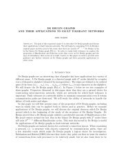
We can now look at a fundamental region defined on H. We let the fundamental region
be the points in H above the semicircle with feet at 0 and 1 and the semicircle with feet at
−1 and 0, and between the infinite vertical lines −1 and 1. The following diagram shows
the fundamental region with a and b drawn in.
1
0.8
0.6
0.4
0.2
–1 –0.8 –0.6 –0.4 –0.2 0 0.2 0.4 0.6 0.8 1
x
2

As shown in [DIW], we can construct the torus as the set of points in this fundamental
region after identifying points on the boundary. Notice that a point is missing (namely the
pointatinfinity); we’ll let this be the puncture.
In particular, each word W ∈ F 2 can be associated with a matrix composed by multiplying
a, b, A, B, whereA and B are the inverses of a and b, respectively. Crisp shows that to find
the number of necessary self-intersections of such a curve, one only needs to count the distinct
number of intersections of cyclic permutations of the word in the fundamental region. [C].
1.2 Simple Loops and the Classification of Curves
One main goal of this research was to create a computer program to perform the tasks stated
above. One would want to enter a word in terms of a, b, and their respective inverses, and
have the program calculate the number of intersections of the geodesics of the axes of matrices
which arise from cyclically permuting the original word. We would then look for obvious
patterns and see why they came about. Also, we hoped that by utilizing this method, we
could easily classify the words that generate 4 necessary self-intersections on the punctured
torus. Also, we wanted to look for any patterns generated when looking at how specific
words generate specific numbers of necessary self-intersections.
Definition 1.3 Two curves on T are equivalent if one is freely homotopic to a curve in the
homeomorphism class of the other.
Definition 1.4 Two words are equivalent if there exists an automorphism in F 2 taking one
curve to the next.
The following theorem relates these definitions. See Section 2 of [CDGISW] for an explanation.
Theorem 1.5 Two curves are equivalent if and only if the words associated with them are
equivalent.
Lemma 1.6 (BCK, Lemma 2.1) Up to free homotopy any loop on T with k transverse
self intersection points can be formed as the composition of k +1 simple loops which intersect
at a single point.
Theorem 1.7 (BCK, Theorem 3.1) Given a generating pair {a, b} for π 1 (T), anyother
generator representable by a simple loop is equivalent to one of the following five,up to orientation
and reflection,
(i) a
(ii) b
(iii) baB
(iv) abA
(v) ab
Using this fact and the Maple program, we can verify all the curves that have 2 necessary
self-intersections by generating a list of curves composed of 3 simple loops and running them
through the program to pick out those with the correct number of intersections.
3

2 Program Data for Equivalence Classes of Curves
Initially, I took a list provided to me by Cooper and Rowland [CR], and input it into the
Maple program. I hoped to find patterns and understand more about how intersections
occurred on the torus. The following is some data that the program returned.
Equivalence Class Intersections
a n , (abAB) n Not a Geodesic, has n − 1 intersections
aaabb 2
aabaB 2
aabAB 1
aaabAb 3
aaabaB 3
aaabbb 4
aaabAB 2
aabaaB 3
aabaBB 4
aabbaB 4
aabbAB 3
aabAAB 2
aaabAAb 4
aaaabaB 4
aaaabbb 6
aaaabAB 3
aaabaaB 4
aaabaBB 6
aaabbaB 6
aaabbAb 6
aaabbAB 5
aaabAbb 6
aaabAAB 3
aaabABB 5
aabaaBB 6
aabbaBB 6
aabbAAB 5
... ...
This is just a sample of the data I received. From this data, I noticed that the maximum
number of intersection given the word length seemed to be predictable. I noticed also
that words of the form a n 2 b n 2 and a n+1
2 b n−1
2 seemed to generate these high numbers. Upon
researching this further utilizing the Maple program, I found the following list and derived
the theorem I show in the following section.
4

Even Words Intersections Odd Words Intersections
a 2 b 2 1 a 2 b 0
a 3 b 3 4 a 3 b 2 2
a 4 b 4 9 a 4 b 3 6
a 5 b 5 16 a 5 b 4 12
a 6 b 6 25 a 6 b 5 20
a 7 b 7 36 a 7 b 6 30
a 8 b 8 49 a 8 b 7 42
a 9 b 9 64 a 9 b 8 56
a 10 b 10 81 a 10 b 9 72
a 11 b 11 100 a 11 b 10 90
3 The Maximum Number of Necessary Self-Intersections
for a Word of Length n
The preceding data suggests a theorem both about the maximal number of transverse intersections
as well as which words, or classes of curves generate this maximum. I shall,
however, prove this in steps.
Theorem 3.1 Let W beawordoflengthn containing j total a’s and A’s, with j ≥ 1 and
n ≥ j +1. Then the necessary self-intersections for W is bounded above by (j −1)(n−j −1).
Proof. Without loss of generality, we can assume that W begins with an a and ends with
a b, by performing automorphisms on W .
Suppose, also that W = a α 1
d β 1
1 c α 2
1 d β 2
2 ...c α k−1
k−1 dβ k−1
k−1 cα k
k
bβ k ,where"ci "and"d i "represent
letters that are either a or b (respectively) or their inverses. In counting the number of
intersections of W , we will assume the worst possible scenario, then show that it is the
boundlistedabove.
I would like to describe a method of viewing curves on the punctured torus. Let the
rectangular object in the next figure represent the punctured torus T. In this case, we let the
corners of the rectangle represent the puncture, and we identify the two sides labelled a and
the two sides labelled b.
5

a
b
b
a
Now, we can represent curves as combinations of a’s and b’s by drawing them as directed
horizontal and vertical lines on this rectangle, as shown in the next two figures. Note that
A and B are lines of the same type, drawn in the opposite direction. Note that a k and b k
can be represented as in the diagrams with complete k − 1 horizontal or vertical segments
and two partial horizontal or vertical segments, respectively.
a
b
.
.
.
b
a
6

a
b
...
b
a
When we look at our word W , we see that we can represent it in terms of horizontal and
verticalbands. Sinceweassumethatwestartwithana and end with a b, wecanbeginto
represent this curve on T by choosing disjoint intervals D 1 ,D 2 , ..., D k and C 1 ,C 2 , ..., C k as
pictured below. The curve will be represented by segments in ∪D i × [0, 1] and [0, 1] × ∪C i .
. . .
C k
C2
. . .
b
D k
. . .
D 2
D 1
C
1
a
We note that these "bands" will be created as sections of horizontal and vertical lines in which
the paths of these lines are traced out alternating (because of the nature of W ). Referring
to the next figure, we can start out at a point which we label 1.
7

4
1
D k
. . .
a
3
2
D 1
C k
. . .
C 2
C1
b
We draw the first part of the curve corresponding to c α 1
1 in [0, 1] × C 1 as pictured above
(beginning at point 1). Note this begins at the lower left of D k ∩ C 1 and ends at the upper
right corner of C 1 ∩ D 1 .1 starts a horizontal line that begins at some point before the left
edge of the rectangle, extends past that edge, and continues on the next horizontal line. This
"looping" around the rectangle continues until we reach our d β 1
1 . Thisnextphaseofthe
curve is marked by "2" and occurs where the corner of the last a meets with this b or B.
Now we continue in this fashion only in the vertical direction.
8

a) b)
.
.. .
.
a -> b
. . . . . .
. . . . . . . . .
.
.
.
a -> B
. . .
.
.
A -> b
.
.
.
.
. . .
.
.
. . .
. . . . . . . . .
A -> B
. . .
c) . . . . . . d)
.
.
.
. . . . . . . . . . . .
e) . . . f)
. . . . . . . . .
g) h)
. . .
. . .
. . .
. . .
. .
. .
. .
.
.
.
b -> a
. . . . . .
. .
. .
.. .
. . . .
.
.
b -> A
B -> A
. . . . . .
. . .
. . .
. . .
. . .
B -> a
.
.
.
. .
. .
. .
. . .
.
.
.
. . .
. . . . . .
The figure above refers to the different types of ways two c i and d i can intersect, excluding the
first and last cases. In each case, you see that each d β i
i intersects the previous c α i
i ,making
α i β i number of intersections.
Again, from the previous figure, note that all of these new vertical lines pass through all
of the horizontal lines, with the exception of one (since 1 and 2 form a line in which there
are no intersecting lines from d β 1
1 . This process continues when we stop at point 3. We go
back to the horizontal lines as defined by c α 2
2 . Note, once again, that these horizontal lines
intersect the previous vertical lines. We can let this process continue until it reaches the
final d β k
k
. We observe that this set of vertical lines starts at point 4 in the figure. Since it
is a b, weknowitwilltravelupward,circlingaroundβ k times, and connecting back to point
1. Notice, though, that there are two partial lines in this group. There is one near 4, and
one that connects back to 1. Thus, only β k − 1 lines intersect all the other horizontal lines.
In short, all horizontal lines, with the exception of the one mentioned, intersect all the other
vertical lines, again, with the exception of one in the last group. So if we simply look at the
intersection of each b with each prior a (excluding the first a and last b), and the intersection
of each subsequent a with each prior b (again excluding the two special cases), we can count
the total number of maximum intersections.
9

Continuing in this manner, let k =1, and we see that the number of intersections of W
is (β 1 − 1)(α 1 − 1), since we disregard the first a and the last b and the b’s must intersect
the a’s in this particular lattice, as defined above. More specifically, if we assume the worst
case, each b must intersect all the a’s prior to it (with the exception of the first a), and all
the a’s must intersect all b’s prior to them. Notice this number matches the bound listed
above.
Suppose k =2, and we see that the number of intersections is β 1 (α 1 − 1) + α 2 β 1 +(β 2 −
1)(α 1 + α 2 − 1) = (α 1 + α 2 − 1)(β 1 + β 2 − 1), thebound.
Checking for k =3, we see the number of intersections is
β 1 (α 1 − 1) + α 2 β 1 +β 2 (α 1 +α 2 −1) + α 3 (β 1 +β 2 )+(β 3 − 1)(α 1 + α 2 + α 3 − 1) = (α 1 + α 2 +
α 3 − 1)(β 1 + β 2 + β 3 − 1); again, the bound. In each case, we see that each exponent above
the a’s is multiplied by each exponent ³X
above the b’s, then we subtract each of these exponents
once and add 1; thisalwaysgivesus (a exponents) − 1´³X
(b exponents) − 1´
.
By induction, we’ll assume that it holds for u that the number of intersections of W =
a α 1
b β 1
a α 2
b β 2
...a α k−1 b
β k−1a α u
b β u
is (α 1 + α 2 + ... + α u − 1)(β 1 + β 2 + ... + β u − 1) = m u . Now
we’ll add an extra a q b p to the end of the word. So the number of intersections of W become
β 1 (α 1 − 1) + α 2 β 1 + β 2 (α 1 + α 2 )+... +(q − 1)(α 1 + α 2 + ... + α u + p − 1) =
m u +b(α 1 +α 2 +...+α u −1)+q(β 1 +β 2 +...+β u )+(p−1)(α 1 +α 2 +...+α u +q −1)+1 =
(α 1 + α 2 + ... + α u + q − 1)(β 1 + β 2 + ... + β u + p − 1); thebound.
Alternatively, we can count this directly by simply looking at the number of intersections
of the "squares" generated by the intersection of each band. We know that the c 1 band
intersects every other d band resulting in at most (α 1 − 1) intersections. Similarly, the d k
band intersects every other c band resulting in at most (β k − 1) intersections. So we can
add the intersections in the following way:
int. ≤ (α 1 −1)(β 1 +β 2 +...+β k −1)+α 2 (β 1 +β 2 +...+β k −1)+...+α k (β 1 +β 2 +...+β k −1)
=(α 1 + α 2 + ... + α k − 1)(β 1 + β 2 + ... + β k − 1), thebound.
Corollary 3.2 Let W beawordoflengthn. Let S W be the minimum number of necessary
self-intersections for a curve represented by W .
Then
½ (
n
2
max{S W } =
− 1)2 ,n even
¡ n+1
¢ 2
− 3 ¡ ¢
n+1
.
2
2 +2,n odd
Proof. By Theorem 3.1, the bound for W is (k − 1)(n − k − 1), withk defined above.
Using n calculus, we find the maximum of this polynomial to be:
¡ o 1 n − 1¢ 2
, at ©£ k = 1n¤ª , as noted above. The only restriction is that n be an
2 2 2
integer; in other words n must be even.
Let us look at the closest value that yields an odd word near the maxima. Since the bound
is a quadratic in k with n fixed, we can differentiate it twice to verify that it is concave down.
Since it is concave down, and has maximum at k = n , we can look at the closest integer
2
values to the maximum: namely n−1 and n+1
n+1
. Consequently, the maximum is at with
2 2 2
value ¡ ¢
n+1 2
− 3 ¡ n+1
2
2
¢
+2.
10

3.1 BackgroundonWordMatricesandSymmetry
To prove the values are realized as described above, we need to look at each of the word
cases (even and odd) separately. First we will introduce some basic principles used in the
proof, then break it up by case.
We let µ a and
b be represented µ by matrices in the form:
1 1
1 −1
a = and b =
.
1 2
−1 2
We will define the inverses of a and b as their respective matrix inverses and denote these
as A and B.
We need only to look at the cyclic permutations of a word W to find the geodesics. Once
we find the types of geodesics created by cyclically permuting W, we can see how many times
these geodesics intersect in the fundamental region.
We will look at specific cases of the cyclic permutations of W :
Even
Odd
W 1 = a n 2 b n 2
W 7 = a n+1
2 b n−1
2
W 2 = b n 2 a n 2
W 8 = b n−1
W 3 = a k b n 2 a n 2 a n+1
2
2 −k
W
W 4 = b k a n 2 b n 9 = a k b n−1
2 −k
2 a n+1
2 −k
W
W 5 = a n 2 −1 b n 10 = b k a n+1
2 b n−1
2 −k
2 a
W 6 = b n 2 −1 W
a n 2 b 11 = a n+1
2 −1 b n−1
2 a
W 12 = b n−1
2 −1 a n+1
2 b
Table 1
To find the geodesics, we multiply the letters of the words using the usual matrix multiplication.
µ Then, once we have a matrix, we can use a transformation defined as:
a b
T : → az + b to transform the matrices to a form from where we can find their
c d cz + d
µ a b
corresponding geodesics. To find these geodesics, we solve the equation z = T ( )
c d
which is quadratic (for all words except W =(abAB) n or W = a n ,W = b n ). The values of
the solutions are the feet of the geodesic, thus all geodesics are in the form of semicircles on
the upper half plane.
Now, lets look at the case where W has n even letters. As suggested by Table 1, many of
the words are symmetric. So W 0 = a n 2 b n 2 is very similar to W 0 = b n 2 a n 2 . To take advantage
of this similarity, we will look at one of the cases, figure out what has changed in the second
case (usually only a sign), then we can apply our knowledge to deduce the second geodesic.
Lemma 3.3 Words of the form a n ,b n , and a n 2 b n 2
µ µ are related to
the Fibonacci number in the
following way: a n F2n−1 F
=
2n
, b
F 2n F n F2n−1 −F
=
2n
,
µ µ 2n+1
−F 2n F 2n+1
and a n 2 b n Fn−1 F
2 =
n Fn−1 −F n
=
µ
F n F n+1 −F n F n+1
−Fn 2 + Fn−1 2 −F n F n−1 + F n F n+1
F n F n−1 − F n F n+1 −Fn 2 + Fn+1
2 ,whereF n denotes the n th Fibonacci number.
11

µ 2 3
As an example, we see that a 2 =
3 5
µ 5 8
,a 3 =
8 13
, all Fibonacci numbers.
Definition 3.4 Let φ = 1+√ 5
, represent the golden ratio.
2
µ
µ
Fn+1
Fn−1
Lemma 3.5 The lim n→∞ = φ, lim n→∞ = 1 φ
F n F n
F n−1
+ F n+1
− φ monotonicallydecreaseto2φ − 1 as n →∞.
F n F n
= φ − 1 and the values of
Lemma 3.6 If W = a n 2 b n 2 , then all cyclic permutations W p1 = a k b n 2 a m and W p2 = b k a n 2 b m
of W have symmetric roots.
Proof. We look at equations of the form W p1 = a k b n 2 a m and W p2 = b k a n 2 b m . Since n
is even, we know that k + m = n , assuming these equations are cyclic permutations of W .
2
Then µ we perform the µ following matrix µ multiplication:
F2k−1 F 2k F2n−1 −F 2n F2m−1 F 2m
=
µ
F 2k F 2k+1 −F 2n F 2n+1 F 2m F 2m+1
F2m (F 2k F 2n+1 − F 2n F 2k−1 )+F 2m−1 (−F 2k F 2n + F 2k−1 F 2n−1 )
F 2m (−F 2k F 2n + F 2k+1 F 2n+1 )+F 2m−1 (F 2k F 2n−1 − F 2n F 2k+1 )
F 2m (−F 2k F 2n + F 2k−1 F 2n−1 )+F 2m+1 (F 2k F 2n+1 − F 2n F 2k−1 )
µ
F 2m (F 2k F 2n−1 −
µ
F 2n F 2k+1 )+F 2m+1
µ
(−F 2k F 2n + F 2k+1 F
2n+1 )
F2k−1 −F 2k F2n−1 F 2n F2m−1 −F 2m
=
µ
−F 2k F 2k+1 F 2n F 2n+1 −F 2m F 2m+1
F2m (F 2k F 2n+1 − F 2n F 2k−1 )+F 2m−1 (−F 2k F 2n + F 2k−1 F 2n−1 )
F 2m (F 2k F 2n − F 2k+1 F 2n+1 )+F 2m−1 (−F 2k F 2n−1 + F 2n F 2k+1 )
F 2m (F 2k F 2n − F 2k−1 F 2n−1 )+F 2m+1 (−F 2k F 2n+1 + F 2n F 2k−1 )
.
F 2m (F 2k F 2n−1 − F 2n F 2k+1 )+F 2m+1 (−F 2k F 2n + F 2k+1 F 2n+1 )
Since the only changes in the matrices are the signs of the upper right and lower left
entries, µ let us assume that the entries are
µ
µ
α β
α β
α −β
, without loss of generality. So W
γ δ
p1 = ,andW
γ δ
p2 =
.
−γ δ
By performing our transformation, we seeq
T (W p1 )=z has roots at − (δ − α) ± (δ − α) 2 +4γβ
, while T (W p2 )=z has roots at
q
2γ
− (δ − α) ± (δ − α) 2 +4γβ
. Since the only difference in these two roots is the lower
−2γ
term’s sign, they are symmetric.
Lemma 3.7 Words with n even, n ≥ 4 of the form W = a n 2 b n 2
[1, ∞).
have roots in [0, 1] and
12

Proof. Using the matrices defined above for a and b, wecansolveforthematrixofW .
µ µ
W = a n 2 b n Fn−1 F
2 =
n Fn−1 −F n
µ
F n F n+1 −F n F n+1
−Fn =
2 + Fn−1 2 −F n F n−1 + F n F n+1
F n F n−1 − F n F n+1 −Fn 2 + Fn+1
2 .
By applying the linear fractional µ transformation
a b
T, we can solve z = T ( )
c d
to get z 2 − (F n−1 + F n+1 )
z +1=0, which has solutions at
F n
v uuut ⎛
(F n−1 + F n+1 ) (F ± 2 n−1 + F n+1 )
⎝
F n
F n
⎞2
⎠ −4
2
=
v uuut ⎛
F n−1 F n+1 F + ± 2 n−1
⎝
F n F n
⎞2
F n+1
+ ⎠ −4
F n F n
.
2
For n =4, (the smallest case), these roots occur at .5657414544 and 1.767591880.
By Lemma 3.5, the roots monotonically come closer to 2φ − 1, so the limit of the roots is
2φ − 1 ±
q(2φ 2 − 1) 2 − 4 2√
5 ± 1
= , since the squared term is a count of distance squared
2
2
(which, by Lemma 3.5, is monotonically decreasing to 2φ − 1. Note the first form of the
root, F n−1
+ F n+1
, will never be lower than it’s first value (again, by Lemma 3.5)).
F n F n
At worst, the lower root is .5657414544, the value above, and it constantly is increasing
towards φ − 1. Similarly, the upper root is at worst 1.767591880, the value above, and
constantly decreasing towards φ. Thus, the values of the roots are in the specified range.
Lemma 3.8 Words with n even, n ≥ 2 of the form W = b n 2 a n 2
[−1, 0].
have roots in (−∞, −1] and
Proof. By symmetry and the previous Lemma.
Lemma 3.9 Words of the form W = b k a n 2 b n 2 −k , 2 ≤ k ∈ Z ≤ n − 2 have roots that follow
the fixed point iteration of G = z − 1
−z +2 .
· ¸ t u
Proof. Let n be given. Without loss of generality, suppose W = . Then
v w
W (z) = tz + u . Suppose the fixed points of W are p and q (i.e. W (p) =p and W (q) =q).
vz + w
Now we wish to cyclically permute W by one bringing one b from the back to the front. So
we’re looking at bW B(x) and we want to find it’s fixed points p 1 ,q 1 such that bW B(p 1 )=p 1
and bW B(q 1 )=q 1 . Noticeifweletx = b(p), wegetbW B(b(p)) = bW (Bb(p)) = bW (p) =
b(p) = p 1 . Then it follows that µ when we bring mb 0 s over to the front of W ,weget
1 −1
p m = b m (p). Now since b =
,b(x) = x − 1
−1 2
−x +2 . In particular, to find the
successive images of p and q, weneedonlytolookattheiterationsoftheb function. Such
a graph follows (b(x) and y=x).
13

4
y
2
–3 –2 –10
1 2 3
x
4 5
–2
–4
Lemma 3.10 Words of the form W = a k b n 2 a n 2 −k , 2 ≤ k ∈ Z ≤ n − 2 have roots that follow
the fixed point iteration of H = z +1
z +2 .
Proof. By symmetry (Lemma 3.6) and by Lemma 3.9.
Lemma 3.11 Words with n ≥ 4, neven of the form W = b n 2 −1 a n 2 b have roots in [−1, 0]
and [1, ∞).
Outline of proof: Take a piece of the word, for instance W 0 = a n 2 −1 b n 2 −1 . Find the
roots of this. The roots start out in (0.565,φ− 1) and (φ, 1.768), by the previous lemma.
By looking at the iteration patterns of the b(x) function, we see that one root converges to
−φ +1, while the other is diverging, and always greater than 1.
Lemma 3.12 Words with n ≥ 4, neven of the form W = a n 2 −1 b n 2 a have roots in [0, 1] and
(−∞, −1].
Proof. By the previous lemma, since W has symmetric roots (Lemma 3.6), the roots of
W = a n 2 −1 b n 2 a are in the negative of the regions of b n 2 −1 a n 2 b.
3.2
14

Words Which Generate the Maximal Number of Necessary Self-
Intersections
Theorem 3.13 The values of Corollary are realized by the words of even length. More
specifically, when n is even, a n 2 b n 2 is such a word that generates the preceding number of
necessary self-intersections.
Proof. We will assume for now that n is even. Because of the symmetry, we can look
at one side of the fundamental region. We know that a n 2 b n 2 has roots that are directed
outside of the fundamental region, so we can disregard it. From the previous lemmas, we
see that one foot of every other geodesic formed from the cyclic permutations of the form
W = b n 2 −k a n 2 b k is in [0, 1]. We also note that the other feet of all of these geodesics are in
[−1, ∞). This means there exists n − 1 geodesics with feet in [0, 1] who’s other feet land
2
past −1. By the symmetry, there exists another n − 1 geodesics with feet in [−1, 0], with
2
feet past 1. Since all of these have radius greater than 1 , we see that they all intersect in
2
the fundamental region. Therefore, they intersect ¡ n
− 2 1¢2 times. A picture of this follows.
2
1.5
1
0.5
–1 –0.6 0 0.2 0.4 0.6 0.8 1
x
Lemma 3.14 For words of odd length, there is a quasi-symmetrical property to the geodesics
in the cyclic permutations of the word. In particular, words of the form a k b n a m , with
k + m = n +1, have roots almost symmetrical to words of the form b k−1 a n+1 b m , a cyclic
permutation of the word. In pairing these "almost symmetrical" words, we see that the
permutation b n 2 a n+1 b n 2 has no symmetrical partner.
Theorem 3.15 The values of Corollary are realized by the words of odd length. More
specifically, when n is odd, a n+1
2 b n 2 is such a word that generates the preceding number of
necessary self-intersections.
15

Outline of Proof: Now a similar situation occurs if the word is of odd length. Since the
word is odd, not all of the cyclic permutations of it have symmetrical counterparts (assuming
the above lemma holds). For example, if W = a 4 b 3 ,weseethatba 4 b has no symmetrical
partner. This means there is one less geodesic with roots near −φ +1and φ. Therefore,
the same lattice structure will occur in the fundamental region, except this time we count
n+1
− 1 intersections from the positive portion of H, and n+1 − 2 intersections from the
2 2
negative portion. These intersect in ¡ n+1
− 1 ¢¡ n+1
− 2 ¢ = ¡ ¢
n+1 2
− 3 ¡ ¢
n+1
2 2 2
2 +2 ways. The
graph below demonstrates this.
2
1.5
1
0.5
–1 –0.6 0 0.2 0.4 0.6 0.8 1
x
4 Miscellaneous Program Data and Observations
When this project began, it was my intent to use my program to check previous work dealing
with classes of curves. In particular, I wanted to verify that specific classes of curves were
the unique classes that generated a specific number of necessary self intersections. To do
this, I would find the possible combinations of k +1 simple loops, make these words minimal
(with the help of [CR]), and run them through my Maple script to ensure only specific classes
of words had k necessary self-intersections. Because of time constraints, I was only able to
verify this for k =2. The following is the theorem we wished to verify.
Theorem 4.1 (DIW, Theorem 3.2) The conjugacy class in π 1 (T) ofalooponT with
two non-trivial self-intersections is one of
(a) [(abAB) 3 ] or [(baBA) 3 ]
(b) [g(aabABabAB)]
(c) [g(abAbaB)]
(d) [g(aaabAB)]
(e) [g(abaBabAB)]
(f) [g(aabAAB)]
16

(g) [g(a 3 )]
(h) [g(aabaB)]
for some g ∈ Aut π 1 (T).
From the list of simple loops (Theorem 1.6), I had Maple generate the list of all possible
combinations of three loops. The following is the list of words the program gave (from
the input of the list of all combinations of three simple loops) that have two necessary
self-intersections:
[{aabaB, aaabAB, aaa, abaBabAB, aabABabAB, aabABab,
abababAB, ababABAB, aabABABAb, aabAb, aabAAB, abaBAB,
aaabABAb, aaabb, aabaBAb, aababb, aabbaBAb, ababaB,
abABabABabAB, ababABabAB}]
After running this through and finding duplicate words, then generating equivalence
classes of the words, we see the list becomes:
[{aabaB}, {aaabAB}, {aaa}, {aabbaBAb, abaBabAB},
{aabABabAB}, {aabAAB}, {aabAb, aaabb}, {abABabABabAB}]
These correspond perfectly with Theorem 3.2 from [DIW].
I also had the opportunity to look at the number of necessary intersections generated
by equivalence classes of words. [CR] generated lists of words by equivalence classes for
words of length up to 15. I was able to analyze these lists using my Maple script up to
word length n =12. The following is the output data from the program. Please note that
the program counts powers of words incorrectly. For instance, the program calculates that
W =(aabaB) 2 has 2 necessary intersections, when it actually has more. This shows that
aabaB has 2 self intersections, and that W traces out this word twice.
Consequently, data below intersection number 7 is inaccurate. To fix this, a procedure
to eliminate words that are powers would need to be implemented.
17

Intersections 1 2 3 4 5 6 7 8 9 10 11 12
0 1 1
1 1 1 1 1 1 1
2 1 2 2 2 1 2 2
3 1 4 2 1 4 2 6
4 1 3 3 4 2 8 3 4
5 1 3 6 7 12 8 6
6 8 2 11 18 16 17
7 9 7 29 40 21
8 12 13 20 34 51
9 6 12 31 64 74
10 24 38 46 97
11 6 40 83 141
12 14 51 95 147
13 28 82 192
14 30 133 208
15 21 56 239
16 9 112 243
17 33 236
18 75 208
19 10 179
20 21 168
21 122
22 85
23 51
24 32
25 14
Conjecture 4.2 Let In
α be the number of equivalence classes for a word of fixed length n
with 0 ≤ α ≤ max{S W },whereα represents the number of necessary intersections for these
classes. Then max {In α } over fixed n occurs where α =2n − 8 and n ≥ 7.
5 Conclusion
We have shown that there is a bound to the number of transverse self-intersections of curves
on the punctured torus. We have also shown that this maximum is realized given certain
types of curves. Though these curves are not the only type in a class represented by words of
an integral length that realize this maximum, they do always generate the maximum number
of self-intersections. The method of representing cuves as geodesics on the hyperbolic upper
half-plane has proven useful, and a good amount of data has been recorded about curves on
the punctured torus. Given more time, one could set out and check the generating classes
for specified numbers of self-intersections for n =3. From there, it would be easy to extend
18

this for n =4or 5. Hopefully patterns will emerge from this and we can easily find the
types of curves that generate a number of intersections, given n.
6 Appendix
The following is the program code I used to produce the desired output in Maple.
The following resets all variables and loads specific packages necessary for the program.
> restart:
> with(linalg):with(ListTools):with(combinat):
stringToList takes in a string. It outputs the string as a list.
Example: stringToList("aabb") yeilds [a,a,b,b].
> stringToList:=proc(Sym)
> local v,q,L,K:
> if evalb(type(Sym, ’symbol’)) then
> K:=convert(Sym, ’string’):
> L:=convert(K, ’list’):
> for q from 1 to nops(L) do
> L[q]:=convert(L[q],’symbol’);
> od
> else
> L:=convert(Sym, ’list’):
> for v from 1 to nops(L) do
> L[v]:=convert(L[v],’symbol’);
> od:
> end if:
> L;
> end proc:
cycPerm takes in a list, and outputs a list of the cyclic permutations of the list.
Example cycPerm([a,a,b,b]) yeilds [[a,a,b,b],[a,b,b,a],[b,b,a,a],[b,a,a,b]].
> cycPerm:=proc(L)
> local i,j,E,M:
> description "Define a set of lists that are cyclic permutations of the original":
> E:={}:
> for i from 0 to nops(L)-1 do
> if i = 0 then
> M[i]:=L:
> else
> M[i]:=Rotate(L,i):
> end if:
> od;
> E:={L}:
> for j from 1 to nops(L)-1 do
19

E:=E union {M[j]}:
> od:
> E;
> end proc:
matMult takes in a list of cyclic permutations and outputs them as a list of matrices
defined by using matrix multiplication to multiply the terms in each list.
Example: matMult([[a,a,b,b],[a,b,b,a],[b,b,a,a],[b,a,a,b]]) yeilds a list of 4 matrices correspondingtomultiplyinga.a.b.b,a.b.b.a,etc.
> matMult:=proc(N)
> global A,B,a,b:
> local j,k,E,m,C:
> description "Cycle through each list (M[i]) and perform the matrix multiplication as
defined by A, B, and their respective inverses":
> a:=Matrix([[1,1],[1,2]]):
> b:=Matrix([[1,-1],[-1,2]]):
> A:=Matrix(inverse(a)):
> B:=Matrix(inverse(b)):
> for j from 1 to nops(N) do
> C[j]:=op(1,op(j,N)):
> for k from 2 to nops(N) do
> C[j]:=C[j] . op(k, op(j,N)):
> od:
> od:
> E:={}:
> for m from 1 to nops(N) do
> E:=E union {value(C[m])}:
> od:
> E;
> end proc:
findGeo takes in a list of matrices, coverts them to functions using the transformation
T(defined below). It will output a list of functions. Each function is equal to the matrix
transformations on the hyperbolic upper half plane. It will error if the trace of a given matrix
is 2 (thus, not equal to a geodesic on the upper half plane).
> findGeo:=proc(H)
> description "Using the transformation T, solve the quadratic to find the geodesic":
> local T, a1,b1,c1,d1,m,F,S,p,rad,cent,l,f,B,w:
> T:=(q,r,s,t)->(q*z+r)/(s*z+t):
> for l from 1 to nops(H) do
> a1:=0:b1:=0:c1:=0:d1:=0:
> #Cycle through each matrix and extract its elements into a1,b1,c1,and d1
> for m from 1 to nops(op(2,H[l])) do
> if [op(1, op(m,op(2,H[l])))] = [1,1] then
> a1:=op(2,op(m,op(2,H[l]))):
> elif [op(1,op(m,op(2,H[l])))] = [1,2] then
> b1:=op(2,op(m,op(2,H[l]))):
20

elif [op(1,op(m,op(2,H[l])))] = [2,1] then
> c1:=op(2,op(m,op(2,H[l]))):
>
> d1:=op(2,op(m,op(2,H[l]))):
> end if:
> od:
> F[l]:=z->T(a1,b1,c1,d1):
> S:=[solve(z=F[l](z))]:
> if abs(trace(H[l])) = 2 then # ERROR HERE: Refer to Dziadosz, Insel, Wiles, REU
1994
> ERROR(‘Particular word entered does not correspond to a geodesic‘):
> end if:
> if evalb(evalf(op(1,S)) > evalf(op(2,S))) then
> p[1]:=op(2,S):
> p[2]:=op(1,S):
>
> p[1]:=op(1,S):
> p[2]:=op(2,S):
> end if:
> if p[2] = p[1] then
> f[l]:=0:
> else
> rad:=(p[2]-p[1])/2:
> cent:=p[1]+rad:
> f[l]:=sqrt(rad^2-(x-cent)^2):
> end if:
> od:
> B:={}:
> for w from 1 to nops(H) do
> B:=B union {f[w]}:
> od:
> B;
> end proc:
iSectFund takes in a list of functions and finds the points where any two intersect in
thefundamentalregion.Itreturnsalistofpoints(x,y)wheretheseintersectionsoccur.
> iSectFund:=proc(f)
> local W, n, idx1, idx2,Pts,intersections,h,xpoint:
> description "Declare h[1] and h[2] as the two geodesics that define the fundamental
region. Find valid intersections in this region":
> intersections:=0:
> Pts:={}:
> h[1]:=sqrt(1/4-(x-1/2)^2):
> h[2]:=sqrt(1/4-(x+1/2)^2):
> #Let W be the different ways we can choose two from the number of specific geodesics
> W:=choose(nops(f),2):
21

#For each element in W, find if the two functions intersect in the fundamental region...count
these by adding 1 to the intersections variable
> for n from 1 to nops(W) do
> idx1:=op(1,op(n,W)):
> idx2:=op(2,op(n,W)):
> if type(solve(f[idx1]=f[idx2]), ’constant’) then
> xpoint:=evalf(solve(f[idx1]=f[idx2])):
> if evalb(xpoint = -1)then
> if evalb(evalf(subs(x=xpoint,f[idx1])) >= 1/2)then
> intersections:=intersections+1:
> Pts:=Pts union {[xpoint,evalf(subs(x=xpoint,f[idx1]))]}:
> else
> if evalb(xpoint >= 0)then
> if evalb(evalf(subs(x=xpoint,f[idx1])) >= evalf(subs(x=xpoint,h[1]))) then
> intersections:=intersections+1:
> Pts:=Pts union {[xpoint,evalf(subs(x=xpoint,f[idx1]))]}:
> end if;
> else
> if evalb(evalf(subs(x=xpoint,f[idx1])) >= evalf(subs(x=xpoint,h[2]))) then
> intersections:=intersections+1:
> Pts:=Pts union {[xpoint,evalf(subs(x=xpoint,f[idx1]))]}:
> end if:
> end if:
> end if:
> end if:
> end if:
> od:
> Pts;
> end proc:
doublePoints takesinalistofpointsofintersectionsandcheckstomakesurethe
points are unique. More specifically, it check points on the boundary and ensures they’re
only counted once. It returns a revised list of points, if need be (a list excluding the duplicate
points).
> doublePoints:=proc(Pts)
> localT,p,newPts:
> description "After initializing the following transformations, check for points on these
fundamental region boundaries. If there are some intersections, perform the transformation
and see if the different representation is in the list. If so, we’ve counted it twice, so subtract
one from the intersections variable.":
> newPts:=Pts;
> T[1]:=z->convert((z+1)/(z+2),float):
> T[2]:=z->convert((z-1)/(-z+2),float):
> for p from 1 to nops(Pts) do
> if op(1,op(p,Pts)) = -1 then
> if member([Re(T[1](-1+op(2,op(p,Pts))*I)),Im(T[1](-1+op(2,op(p,Pts))*I))], Pts) then
22

newPts:=newPts minus {[Re(T[1](-1+op(2,op(p,Pts))*I)),Im(T[1](-1+op(2,op(p,Pts))*I))]}:
> end if:
> end if:
> if op(1,op(p,Pts)) = 1 then
> if member([Re(T[2](1+op(2,op(p,Pts))*I)),Im(T[2](1+op(2,op(p,Pts))*I))], Pts) then
> newPts:=newPts minus {[Re(T[2](1+op(2,op(p,Pts))*I)),Im(T[2](1+op(2,op(p,Pts))*I))]}:
> end if:
> end if:
> od:
> newPts;
> end proc:
iNum takes in a word as either a string or a list, and a parameter Y. It runs the
word through the previous functions. If Y="number", the program returns the number of
intersections in the fundamental region. If Y is anything else, iNum will return a graph of
the functions in the fundamental region. An example follows.
> iNum:=proc(R,Y)
> local P,Q,L,G,H,J,K,E,v:
> #unassign(’A’,’B’,’a’,’b’):
> if evalb(type(R, ’string’)) then
> P:=stringToList(R):
> elif evalb(type(R, ’symbol’)) then
> Q:=convert(R, ’string’):
> P:=stringToList(Q):
>
> P:=R:
> end if:
> G:=cycPerm(P):
> H:=matMult(G):
> J:=findGeo(H):
> K:=iSectFund(J):
> L:=doublePoints(K):
> if Y = "number" then
> nops(L);
> else
> E:={}:
> for v from 1 to nops(J) do
> E:=E union {op(v,J)}:
> od:
> E:=E union {x=1,x=-1,sqrt(1/4-(x-1/2)^2),sqrt(1/4-(x+1/2)^2)}:
> plot(E,x=-1..1, scaling=constrained);
> end if;
> end proc:
Example of iNum:
> W:=aabb;
W:=aabb
23

iNum(W,"number");
1
> iNum(W,"graph");
1.6
1.4
1.2
1
0.8
0.6
0.4
0.2
–1 –0.8 –0.4 0 0.2 0.4 0.6 0.8 1
x
References
[DIW]
Susan Dziadosz, Thomas Insel, Peter Wiles. Geodesics with Two Self-Intersections
on the Punctured Torus. Proceedings of the REU Program in Mathematics. Oregon
State University. September 1994.
[C] David J. Crisp. The Markoff Spectrum and Geodesics on the Punctured Torus,
PhD Theses. University of Adelaide, 1993.
[CDGISW] D. Crisp, S. Dziadosz, D. Garity, T. Insel, T. Schmidt, and P. Wiles. Closed
Curves and Geodesics with Two Self-Intersections on the Punctured Torus. Mh.
Math. 125, 189-209 (1998).
[BCK]
MandeButler,JeanneCarton,EmilKraft. Geodesics with Three Intersections on
the Punctured Torus. Proceedings of the REU Program in Mathematics. Oregon
State University. September 1995.
[CR] Bobbe Cooper and Eric Rowland. On Equivalent Words in the Free Group on
Two Generators. Proceedings of the REU Program in Mathematics. Oregon State
University. August 2002.
[H]
Kevin Hare. Fixed Point Iteration in Maple.
http://www.cecm.sfu.ca/~kghare/numeric/fixed_point.html.
Accessed 08/07/2002.
24