Geometric Facility Location Problems
Geometric Facility Location Problems
Geometric Facility Location Problems

Create successful ePaper yourself
Turn your PDF publications into a flip-book with our unique Google optimized e-Paper software.
Pinaki Mitra<br />
Dept. of CSE<br />
IIT Guwahati
Heron’s Problem<br />
• HIGHWAY FACILITY LOCATION<br />
<strong>Facility</strong><br />
High Way<br />
Farm A<br />
Farm B
Illustration of the Proof of Heron’s<br />
Theorem<br />
p<br />
q<br />
s<br />
r<br />
r’ l<br />
d(p,r) + d(q,r) = d(p’,q)<br />
p’<br />
d(p,r’) + d(q,r’) = d(p’,r’) + d(q,r’) >= d(p’,q)
MINIMAX FACILITY LOCATION<br />
Given n points in the plane representing customers<br />
(plants, schools, towns etc..) it is desired to determine<br />
the location X (another point in the plane) where a<br />
facility should be located so as to minimize the<br />
distance from X to its furthest customer.<br />
The problem has an elegant and succinct geometrical<br />
interpretation: “Find the smallest circle that encloses a<br />
given set of n points.”<br />
The center of the circle is<br />
Precisely the location of X<br />
+<br />
The smallest<br />
circle enclosing a<br />
set of points
The minimum enclosing circle can be computed from<br />
the Furthest Neighbor Voronoi Diagram. [Shamos]<br />
The correctness of the above algorithm was<br />
established by [Bhattacharya & Toussaint]. Their<br />
argument is based on the following property of the<br />
minimum enclosing circle :<br />
The minimum enclosing circle of a set S of n points is<br />
either determined by the diameter of the point set S or<br />
by three points on the convex hull of S, where those<br />
three points form an acute angled triangle.
Furthest Neighbor Voronoi Diagram can be<br />
computed from the projection of the upper hull of the<br />
point set lifted on the paraboloid z = x 2 + y 2 .<br />
z<br />
q<br />
(x 1<br />
,y 1<br />
, x 12<br />
+y 12<br />
))<br />
y<br />
p<br />
(x 1<br />
,y 1<br />
)<br />
(x,y) (x,y, x 2 +y 2 )<br />
x
But the computation of Furthest Neighbor Voronoi<br />
Diagram is lower bounded by the computation of the<br />
convex hull of n points i.e., Ω (nlogn).<br />
But this lower bound doesn’t hold for the minimum<br />
enclosing circle.<br />
In fact we can compute the minimum enclosing circle<br />
of a set of n points in θ(n) time by solving three<br />
variable Convex Program. [Meggido]<br />
The result holds for any fixed dimensional point set.
Here (x 1<br />
,y 1<br />
), (x 2<br />
, y 2<br />
), …., (x n<br />
,y n<br />
) are the set of points for which we have to<br />
compute the minimum enclosing circle.<br />
Let (x,y) be the center of the minimum enclosing circle and let r be its radius.<br />
Then we have the minimum enclosing circle problem formulated as the<br />
following optimization problem:<br />
Minimize r 2<br />
Subject to: (xx i<br />
) 2 + (yy i<br />
) 2 ≤ r 2 i = 1, 2, …, n<br />
If we substitute z = x 2 + y 2 – r 2 then we have the following convex<br />
programming formulation of the problem:<br />
Minimize x 2 + y 2 – z<br />
Subject to: 2xx i<br />
2yy i<br />
+ z + (x i<br />
2<br />
+ y i2<br />
) ≤ 0 i = 1, 2, …, n<br />
Thus we have to minimize a quadratic function over a set of linear<br />
constraints involving 3 variables.
FermatWeber Problem<br />
Problem Definition:<br />
For a given set of m points x 1<br />
, x 2<br />
, …, x n<br />
with each x i<br />
∈ R d find a<br />
point y from where the sum of all Euclidean distances to the x i<br />
’s<br />
is the minimum.<br />
This problem is also known as <strong>Geometric</strong> 1Median problem :<br />
arg min<br />
n<br />
∑<br />
d<br />
y ∈ R i=<br />
1<br />
x<br />
i<br />
−<br />
y<br />
The special case when n = 3 and d = 2 arises in the<br />
construction of Minimal Steiner Trees and was originally<br />
posed as problem by Torricelli.
a<br />
f<br />
120°<br />
b<br />
c<br />
For 3 coplanar points a, b, c if each angle of the triangle abc is less tan 120 ° the<br />
Fermat Point f is a point inside the triangle which subtends 120° an angle to all<br />
three pairs of points. Otherwise if any angle of the triangle abc is greater than<br />
then Fermat Point is the point making that angle.<br />
For 4 coplanar points if a point is inside the triangle formed by the other three<br />
points then geometric 1median is that point. Otherwise all 4 points form a<br />
convex quadrilateral and the geometric 1median is the intersection point of<br />
both the diagonals and also known as Radon Point.<br />
1 med
If we restrict d = 1 , i.e., for the 1dimensional case then the geometric 1<br />
median coincides with the median.<br />
Again if we consider the problem in L 1<br />
metric with d = 2, i.e., in 2dimension<br />
we can combine the optimal solutions of two 1 dimensional problems to<br />
obtain the optimal solution of the original problem.<br />
x<br />
The method extends for any value of d in L 1<br />
metric ,i.e., we can decompose<br />
the problem in d one dimensional problems and combine their optimal<br />
solution to obtain the optimal solution of the original problem.<br />
In L 2<br />
metric Weiszfeld’s algorithm iteratively computes the geometric 1<br />
n<br />
median problem : x<br />
y<br />
i+<br />
1<br />
y<br />
∑<br />
j=<br />
1<br />
= n<br />
∑<br />
j=<br />
1<br />
x<br />
x<br />
j<br />
j<br />
j<br />
−y<br />
1<br />
−y<br />
i<br />
i
KMedian<br />
Given a set S of n points in the plane we have to locate a set F of k facilities<br />
that partitions the set S in k partitions N(f i<br />
) i =1,2, …, k so that for any site s j<br />
∈ N(f i<br />
) [neighborhood of f i<br />
] being served by the facility f i<br />
the following sum<br />
is minimized:<br />
k<br />
∑<br />
∑<br />
i= 1 s ∈N<br />
( )<br />
j f i<br />
dist(<br />
f<br />
i<br />
,<br />
s<br />
j<br />
)<br />
where<br />
S<br />
=<br />
k<br />
N(<br />
f i<br />
)<br />
i=<br />
1<br />
and<br />
N( f ) N(<br />
f ) = φ,<br />
1≤<br />
i<br />
j<br />
i<br />
<<br />
j<br />
≤<br />
k
In kmedian problem the elements for the set F can be any k<br />
sites in R d in the unrestricted case. Sometimes we restrict the<br />
kmedian problem such that F ⊆ S, i.e., input point sites. Both<br />
of these problems are NPHard. [Meggido & Supowit]<br />
So our goal should be the design of efficient approximation<br />
algorithms for these problems. Here we will restrict our attention<br />
to the restricted version of the problem.<br />
Restricted version of our facility location can still be classified<br />
into two subcategories:<br />
(a) Uncapacitated kmedian problem<br />
(b) Capacitated kmedian problem
A common assumption used when dealing with location problems is that<br />
facilities are uncapacitated and can thus service any number of demand<br />
destinations. But the assumption may be unrealistic in many applications<br />
and thus in capacitated facility location an upper bound is provided on the<br />
number of demand destinations serviced by each facility.<br />
Now we can formulate these problems using ILP as follows:<br />
Minimize<br />
n<br />
∑<br />
i=<br />
1<br />
n<br />
∑<br />
j=<br />
1<br />
dist ( s , s ) x<br />
i<br />
j<br />
ij<br />
Subject to:<br />
n<br />
∑ x ij<br />
= 1<br />
i=<br />
1<br />
n<br />
∑x<br />
ij<br />
≤<br />
j=1<br />
C<br />
i<br />
j =1,2,...,<br />
i =1,2,...,<br />
n<br />
n<br />
n<br />
∑i<br />
y = k<br />
i=1<br />
y<br />
i<br />
− x ij<br />
≥ 0<br />
i =1,2,...,<br />
n<br />
j =1,2,...,<br />
n
y i<br />
∈{0,1}<br />
xij<br />
∈{0,1}<br />
i = 1,2,...,<br />
n j =1,2,...,<br />
n<br />
The indicator variable y i<br />
denotes if the site s i<br />
is selected as<br />
the facility or not.<br />
The indicator variable x ij<br />
denotes if the facility at the site s i<br />
serves the customer at site s j<br />
.<br />
Since ILP is NPComplete the usual technique is to relax the<br />
integrality constraint , i.e., replace the above two constraints<br />
by:<br />
0 ≤ y ≤ 1<br />
0 x ≤1<br />
≤ ij<br />
i<br />
i =1,2,...,n<br />
i = 1,2,...,<br />
n j =1,2,...,<br />
n
Then we solve the LPrelaxation of the ILP. After that the<br />
fractional solution is cleverly rounded maintaining the feasibility<br />
and some bound is established w.r.t Z* LP<br />
≤ Z* ILP<br />
For rectilinear 1median problem Ω(nlogn) lower bound was<br />
established by [Bajaj].<br />
As far as upper bounds are concerned there are O(n 1.5 log 4 n)<br />
time algorithm for arbitrary weighted points and O(nlog 4 n) time<br />
algorithm for equally weighted point set was exhibited by<br />
[ElGindy & Keil]<br />
Thus even in L 1<br />
metric there are big gaps between these upper<br />
and lower bounds.<br />
All these pose several new directions of future research.
Line <strong>Facility</strong><br />
In many practical applications we may be interested in locating<br />
a line facility rather than locating a point facility.<br />
For example we may have to construct a road in some<br />
residential area so that it is convenient to most of the residents.<br />
Then this road design is the same as locating a line facility<br />
among a set of sites for residents.<br />
There can be many variations of these problems in various<br />
metric. The L 2<br />
approximation of this problem, i.e., where we<br />
have to minimize the sum of the squares of the perpendicular<br />
distances is the well known Regression Line Problem.
Given a set of data points (x 1<br />
, y 1<br />
), (x 2<br />
, y 2<br />
), …., (x n<br />
, y n<br />
) we have to find the<br />
equation of the straight line y = ax + b that minimizes the L 2<br />
error, i.e.,<br />
Minimize<br />
Here the variables are in fact a and b. So we have two unknowns and we<br />
require at least two equations to solve. They are obtained from the minima<br />
criterion after taking partial derivatives w.r.t. a and b respectively:<br />
The result can be extended for any dimensional data. For example in d<br />
dimensions we have to find the Regression Hyperplane a 1<br />
x 1<br />
+ a 2<br />
x 2<br />
+ … +<br />
a d<br />
x d<br />
= b. Thus we have to<br />
Minimize<br />
n<br />
∑<br />
i=<br />
1<br />
2<br />
[ yi − ( axi<br />
+ b)]<br />
=<br />
n<br />
∑<br />
i=<br />
1<br />
d<br />
[ b − ∑<br />
j=<br />
1<br />
a<br />
j<br />
∂E<br />
∂a<br />
x<br />
i<br />
j<br />
]<br />
2<br />
E<br />
∂E<br />
= 0 , = 0<br />
∂b<br />
=<br />
E
Thus we have d unknowns a 1<br />
, a 2<br />
, …, a d<br />
. They are solved from the following<br />
system of equations:<br />
∂E<br />
∂a<br />
1<br />
∂E<br />
= 0,<br />
∂a<br />
2<br />
∂E<br />
= 0,...,<br />
∂<br />
a d<br />
= 0<br />
For L 1<br />
approximation of the problem we have to<br />
Minimize<br />
n<br />
∑<br />
i=<br />
1<br />
| b<br />
d<br />
−∑<br />
j=<br />
1<br />
a<br />
j<br />
x<br />
i<br />
j<br />
| =<br />
E<br />
This absolute value function is not a linear function. But we can easily<br />
convert it to a standard LP problem as follows [Chvatal]:<br />
Minimize<br />
Subject to:<br />
n<br />
∑<br />
i=<br />
1<br />
b<br />
e i<br />
d<br />
−∑<br />
j=1<br />
−b<br />
+<br />
d<br />
j=1<br />
a<br />
∑<br />
j<br />
a<br />
j<br />
x<br />
x<br />
i<br />
j<br />
i<br />
j<br />
≤ e<br />
i<br />
≤ e<br />
i<br />
i =1,2 ,...,<br />
i =1,2 ,...,<br />
n<br />
n
For L ∞<br />
approximation of the problem we have to<br />
Minimize<br />
max<br />
i<br />
| b −<br />
d<br />
∑<br />
j=<br />
1<br />
a<br />
j<br />
x<br />
i<br />
j<br />
|<br />
This can be directly formulated into LP as follows:<br />
Minimize<br />
z<br />
Subject to:<br />
z<br />
d<br />
+∑a<br />
j<br />
x ≥b<br />
j=1<br />
i<br />
j<br />
i =1,2 ,...,<br />
n<br />
z<br />
d<br />
−∑<br />
j=1<br />
a<br />
j<br />
x<br />
i<br />
j<br />
≥−b<br />
i =1,2 ,...,<br />
n<br />
The problem of L 1<br />
and L ∞<br />
approximation problem was first posed<br />
By Fourier. Subsequently many good algorithms for computing L 1<br />
and L ∞<br />
approximation were proposed by [Bloomfield & Steiger].
Similar type of problems for line facility concerns:<br />
i) Locating a line facility that minimizes the maximum distance<br />
from a set of sites.<br />
ii) Locating a line facility that minimizes the sum of the distances<br />
from a set of sites.<br />
There are several possible extensions of these problems.