Lecture 3: Total Station and GPS Surveys
Lecture 3: Total Station and GPS Surveys
Lecture 3: Total Station and GPS Surveys

Create successful ePaper yourself
Turn your PDF publications into a flip-book with our unique Google optimized e-Paper software.
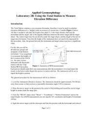
Applied Geomorphology<br />
<strong>Lecture</strong> 4: <strong>Total</strong> <strong>Station</strong> & <strong>GPS</strong><br />
Survey Methods
<strong>Total</strong> <strong>Station</strong><br />
• Electronic version of Alidade<br />
• Accurate to ±3 ppm horizontal & vertical<br />
–3x10 -6 (5000 feet) = 0.2 inches
<strong>Total</strong> <strong>Station</strong> Advantages over the<br />
Alidade<br />
• Calculations are processed internally so there<br />
are no post data collection calculations to<br />
process<br />
• Accuracy is much better than alidade, <strong>and</strong> it is<br />
not shot distance dependent<br />
• Results are stored in a data collector computer<br />
that can display results graphically<br />
• Each individual ray shot can take as little as a<br />
few seconds to take- many more stations can be<br />
collected per day as compared to the alidade<br />
<strong>and</strong> plane table method
<strong>Total</strong> <strong>Station</strong> Disadvantages<br />
• No plane table for sketching contours<br />
<strong>and</strong>/or contacts on a geologic map<br />
• It may take 30 minutes to an hour to set up<br />
(level) the instrument before data can be<br />
collected<br />
• Battery life on data collector computer can<br />
limit length of daily surveys
<strong>Total</strong> <strong>Station</strong> <strong>Surveys</strong><br />
• The initial XY coordinate system of the<br />
instrument is r<strong>and</strong>om- it must be calibrated to<br />
conform to geographic or magnetic north<br />
• A “backsight” target is established north of the<br />
starting station position to calibrate coordinate<br />
system<br />
• If two benchmarks or former station positions<br />
have known coordinates the relative positions<br />
can be used to calibrate coordinate system<br />
• Because of the range <strong>and</strong> accuracy of the total<br />
station one instrument station may be sufficient<br />
for entire survey project
Integrating Pocket Transit & <strong>Total</strong><br />
<strong>Station</strong> <strong>Surveys</strong><br />
• To integrate a Transit survey with T.S.<br />
data you must “grid” the transit points<br />
based on the XY coordinates of two known<br />
points.<br />
• Once grid lines are established on the<br />
alidade map each data point is read off as<br />
if the map were a sheet of graph paper.
Integrating Transit & T.S. <strong>Surveys</strong><br />
• Campus Map Example using stations 1 & 2<br />
St1 = 5000, 5000 (measured w/ T.S.)<br />
St2 = 4984, 4744 (measured w/ T.S.)<br />
∆x= 16, ∆y = 256<br />
Tan α = ∆x / ∆y = 16/256 5000<br />
α = 3.6°<br />
Ray1 = 4819, 5067<br />
(interpolated from grid)<br />
4900<br />
4800<br />
4900 5000 5100<br />
Ray1<br />
86.4°<br />
St1<br />
3.6°<br />
4800<br />
St2
<strong>GPS</strong> <strong>Surveys</strong><br />
• Global Positioning System<br />
• Constellation of 24 satellites orbiting at<br />
50,000 km altitude<br />
• At a given point on the earth at least 4<br />
satellites can be tracked by receiver<br />
simultaneously<br />
• 3 satellites plus the earth define a range of<br />
possible positions; the 4 th satellite timing is<br />
used to arrive at a consistent position
Earth- <strong>GPS</strong> Satellite Geometry<br />
Earth
<strong>GPS</strong> Satellite Characteristics<br />
• Contain a very accurate atomic clock<br />
• Orbit at a high altitude so that no friction<br />
with the atmosphere is possible, resulting<br />
in a very predictable orbit<br />
• Broadcast signal contains the position of<br />
the satellite, <strong>and</strong> the time the signal was<br />
broadcast<br />
• Satellites are maintained by the Military<br />
<strong>and</strong> NASA
<strong>GPS</strong> Error Sources<br />
• SA: selective availability<br />
• Atmospheric heterogeneity<br />
• Clock Error<br />
• Multipath Error (largest source of error)<br />
• PDOP: position dilution of precision<br />
• Because of satellite geometry z accuracy<br />
is usually 1.5 to 2 times that of horizontal<br />
map accuracy
<strong>GPS</strong> Receiver Types<br />
• Autonomous<br />
– H<strong>and</strong> held receivers with built-in<br />
antenna ($150 - $500)<br />
– Receiver <strong>and</strong> external antenna<br />
(usually as a backpack or harness)<br />
combo ($500 - $5,000)<br />
• Base <strong>Station</strong> (Survey Grade; Real-<br />
Time Kinetic) ($20,000 to $50,000)<br />
– Receiver <strong>and</strong> PDA data collector<br />
– Base station receiver with differential<br />
correction beacon broadcast
Typical <strong>GPS</strong> Accuracy<br />
• Low-end autonomous: 5m (with differential<br />
beacon)<br />
• High-end autonomous: 2m (with differential<br />
beacon)<br />
• RTK: 1cm
Differential Correction Beacons<br />
• A <strong>GPS</strong> receiver is permanently fixed at a known<br />
benchmark<br />
• A correction factor that accounts for the<br />
differential between the actual <strong>and</strong> calculated<br />
position is continually broadcast on the FM radio<br />
b<strong>and</strong> from the benchmark<br />
• In theory any errors generated by PDOP or<br />
atmospheric conditions can be eliminated by a<br />
<strong>GPS</strong> receiver that applies the correction factor<br />
• Multipath errors are not eliminated by differential<br />
beacons (D<strong>GPS</strong>)
<strong>GPS</strong> Accuracy & Precision<br />
• Precision is the reproducibility of the<br />
measurement<br />
• Accuracy is how close the measured<br />
position is to the actual location
Concept of Precision & Accuracy<br />
Good precision,<br />
Poor accuracy<br />
Good precision,<br />
Good accuracy<br />
Poor precision,<br />
Poor accuracy<br />
Poor precision,<br />
Good accuracy
Accuracy & Precision cont.
<strong>GPS</strong> RMS Values<br />
• RMS: root mean<br />
square<br />
• RMS = Σ(d)/N where d<br />
= distance from actual<br />
position
<strong>Lecture</strong> Test 1 Review<br />
• Take home test<br />
• Contour problem: from spot elevations<br />
• Closed traverse: plot from data; adjust error<br />
• Topographic profile: calculate V.E.<br />
• H<strong>and</strong>-Level/Height calculation problem<br />
• ArcGIS contour problem: Grid given data <strong>and</strong><br />
generate contours<br />
• Relational fraction (RF) problems<br />
• Map Coordinate systems (UTM, LOGS, SPCS,<br />
Lat-Long): find map features given coordinates<br />
<strong>and</strong> vice versa.