DEMETER â Autonomous Field Robot
DEMETER â Autonomous Field Robot
DEMETER â Autonomous Field Robot

Create successful ePaper yourself
Turn your PDF publications into a flip-book with our unique Google optimized e-Paper software.
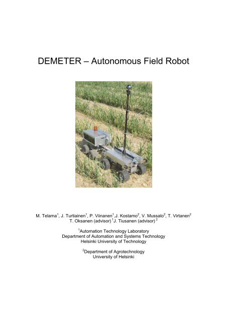
<strong>DEMETER</strong> – <strong>Autonomous</strong> <strong>Field</strong> <strong>Robot</strong><br />
M. Telama 1 , J. Turtiainen 1 , P. Viinanen 1 ,J. Kostamo 2 , V. Mussalo 2 , T. Virtanen 2<br />
T. Oksanen (advisor) 1 J. Tiusanen (advisor) 2<br />
1 Automation Technology Laboratory<br />
Department of Automation and Systems Technology<br />
Helsinki University of Technology<br />
2 Department of Agrotechnology<br />
University of Helsinki
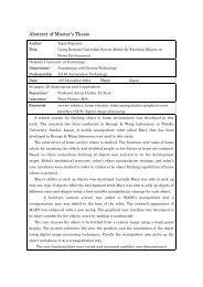
Abstract<br />
An autonomous robot Demeter was developed for the <strong>Field</strong> <strong>Robot</strong> Event 2006.<br />
The four-wheel driven robot was built on a modified RC-platform. Spring<br />
suspension has been replaced with a middle joint. The robot has been build<br />
symmetric, and having all the wheels turning, is equally capable of driving into<br />
either direction. The robot has been made out of aluminum and is battery driven.<br />
The robot is controlled by two microcontrollers and a laptop that all onboard. The<br />
basic tasks for the robot are; driving towards a flag, driving between rows and<br />
hole detection in grass. The robot archives this by using machine vision and<br />
ultrasonic sensors. An electronic compass was included as an additional sensor.<br />
Machine vision uses a webcam attached to a servo that rotates the camera to<br />
point the robot’s driving direction. The robot comes with a trailer that measures<br />
soil hardness and moisture. The work was done by a group of students from two<br />
universities during the semester 2005-2006. This document describes the<br />
development and technology overview of the robot.<br />
Keywords<br />
<strong>Field</strong> robot, Machine vision, autonomous navigation<br />
1. Introduction<br />
In August 2005 a group of six students began planning the building of a robot<br />
that would take part of the <strong>Field</strong>robot competition 2006 in Hohenheim. A similar<br />
team from the same universities had taken part in <strong>Field</strong>robot competition in 2005<br />
under the name Smartwheels. After sharing information with this team, it was<br />
concluded that building the robot should start from a clean table. This time, a<br />
considerable amount of effort was put into planning and designing the robot.<br />
Number of different design possibilities were evaluated, before choosing the<br />
current design. Great care was put into building the mechanics platform to<br />
perform as well as possible. This delayed the project and it was not until April<br />
that the first tests could begin. That and various unexpected problems kept the<br />
team occupied to the last minute.
2. Materials and methods<br />
2.1 Hardware<br />
2.1.1 Chassis<br />
The main task of the chassis of the robot is simple: It should be able to carry the<br />
measurement devices and provide the robot the ability to operate in field<br />
conditions. There are numerous different ways to achieve this goal and the<br />
selection of the technical solution depends on many factors. At least following<br />
properties of the chassis are desirable:<br />
• Reliability<br />
• Low cost<br />
• Good off-road properties<br />
• Good accuracy and ability to respond to instructions<br />
• Low power consumption<br />
In practice the low budget of student project forces to some trade offs and all of<br />
these properties can not often be fulfilled in the desired way. However, it should<br />
be kept in mind that the chassis of the robot is the base on which the all the<br />
sensor and computer systems are built. It is obviously essential requirement that<br />
the chassis is able to drive all the equipment to the position defined by the<br />
controlling computer.<br />
The position of the robot and the position defined by the computer are not the<br />
same due to measurement errors and perturbations. There are many sources of<br />
perturbations when the robot operates in the field. Error to the dead reckoning<br />
position measurement can be caused by e.g. inaccuracies in wheel angles, slip<br />
of the wheels, errors in rotation measurements of the wheels and so on. These<br />
errors cumulate when driving the robot for a longer time in the field and therefore<br />
additional position measurement and navigation systems are needed. Despite of<br />
the additional navigation systems the off road properties of the chassis and its<br />
ability to follow control signal have a significant impact on the performance of the<br />
robot. It is not reasonable to compensate the large errors caused by the chassis<br />
with a sophisticated computer control program. If the errors caused by the<br />
chassis can be kept as small as possible, the reliability of the navigation and<br />
accuracy can be improved. The key point in developing the motion system of the<br />
robot is to ensure good controllability in all conditions that can be normally<br />
expected in the field.<br />
The chassis for the robot is based on a Kyosho Twin Force R/C monster truck.<br />
Building began with the original chassis which needed some modifications, but<br />
eventually a completely new chassis was build. Only the tires, axles and some<br />
parts of the power transmission were kept in the final version of the robot.<br />
The chassis is newly built with self-made parts with no previous drawings, though<br />
based loosely to the original Twin Force parts. Aluminium was chosen because
of its lightness. The engine rooms have been separated from the rest of the<br />
chassis and the microcontrollers have been placed into a separate slot to allow<br />
easy access. Chassis is four-wheel-driven and each one of the engines powers<br />
one axle. All of the springs have been removed, and instead there is a large joint<br />
in the middle of the chassis providing the robot manoeuvrability somewhat similar<br />
to farm tractors.<br />
The vehicle is electrically driven with two Mabuchi 540 motors. The motors are<br />
driven by two PWM amplifiers.<br />
Figure 1 Motor and steering unit<br />
The Motor unit of the Twin Force monster truck was modified to meet the<br />
requirements of the field robot. Two separate motor units were used for both front<br />
and rear axis. The motor units were identical and they were operated<br />
independently from each other. The use of two motor units enables the<br />
independent velocity control and independent steering of both front and rear axis.<br />
The main modifications done to the motor unit were:<br />
• The maximum speed of the Monster truck was reduced to one quarter by<br />
adding an additional pair of gears.<br />
• An optical encoder was attached directly to the shaft of the Mabuchi drive<br />
motors.<br />
• A steering servo was attached to the motor unit<br />
The chassis didn't originally have four-wheel-steering, so it had to be build with<br />
optional parts provided by Kyosho. Four-wheel-steering was necessary to give<br />
the robot enough turning radius. Two HS-805BB+ MEGA servos were used for<br />
steering and they seemed to provide enough steering power for the robot.
Figure 2 Power supply<br />
Eight (8) pieces of 1.2V rechargeable Ni-Mh batteries soldered in series were<br />
used as the power supply of the robot. The capacity of each battery ranged from<br />
7000 mAh to 9000 mAh depending on the battery package that was in use. The<br />
power from the batteries was proven to be adequate.<br />
2.1.2 Sensors and machine vision<br />
Four Devantech SRF08 ultrasonic sensors were used together with a Devantech<br />
CMPS03 I2C compatible compass. The sensors were connected to I 2 C sensor<br />
bus. For machine vision the robot has a Logitech QuickCam Pro 5000 camera<br />
attached to a carbon fibre pole with a servo motor to enable a turn of 180<br />
degrees. The compass was placed to the camera pole, high enough to avoid<br />
magnetic fields that would create interference with it.<br />
2.2 Processing equipment<br />
2.2.1 Microcontrollers<br />
The robot has two microcontrollers: ATMEGA 128 and a PIC 18F2220. The first<br />
one was used to control the Msonic power controllers for the DC-motors, steering<br />
servos, and the camera-servo. The second one was used to collect sensor input<br />
from compass, ultrasonic sensors, and to connect to trailer’s inputs and outputs.<br />
2.2.2 Laptop<br />
A P4 laptop was used to process all necessary tasks along with the<br />
microcontrollers.
2.3 Hardware for the freestyle<br />
2.3.1 Trailer<br />
The trailer was built from scratch. The platform had to be made big enough to fit<br />
all of the equipment and with enough ground clearance to give the linear motor<br />
enough room to function. Old Tamiya Clod Buster wheels were used together<br />
with a new spindle that was made to increase manoeuvrability.<br />
The main equipment used in the trailer is a linear motor provided by Linak. All the<br />
electronics have been fitted into two boxes. The linear motor is operated by two<br />
relays. The primary idea for the freestyle was to measure the penetration<br />
resistance of the soil (cone-index) and simultaneously measure the moisture of<br />
soil by measuring the electrical conductivity of the soil.<br />
The linear motor was used to thrust two spikes into soil. Soil penetration<br />
resistance could then be measured from the amount of current consumption<br />
changes in the linear motor. Simultaneously the electrical conductivity of the soil<br />
was measured with an input voltage of 5V directly from the microcontroller of the<br />
robot. This was an experiment and it has to be remembered that the soil<br />
conductivity measurements rely heavily on other properties of the soil, especially<br />
on the amount of different salts there are in the soil.<br />
The linear motor operates with a 12 V lead-acid battery, which, although being<br />
quite heavy, doesn't give the trailer enough mass to thrust into hard soil.<br />
However the trailer cannot be too heavy for it has to be pulled by the robot. The<br />
weight of approximately 9 kilograms was rather easily pulled.<br />
3. Camera & Machine vision<br />
3.1 Camera<br />
Logitech QuickCam Pro 5000 was used for machine-vision. It's a higher end<br />
webcam, which is still quite cheap. Camera is capable of 640*480 resolution, but<br />
320*240 resolution was used to improve performance and this doesn't require so<br />
much data transfer. Camera sends about 25 images per second to laptop.<br />
Laptop processes about 20 images per second and calculates parameters and<br />
image convertions for each frame.<br />
3.2 Machine vision<br />
Machine vision software was developed on Microsoft Visual C++ 2005 and Open<br />
Source Vision Library ( OpenCV [1] ). OpenCV provides libraries and tools for<br />
processing captured images.
3.3 Preprocessing<br />
Image processing was done by EGRBI [2] color transformation (Excess Green,<br />
Red-Blue, Intensity). At the beginning of algorithm, image is split into 3 spaces:<br />
red, green and blue. In EGRBI transformation a new image-space is created.<br />
Components are Green, Intensity and Red-Blue (cross product of green and<br />
intensity). Intensity is 1/3(R+G+B value).<br />
EGRBI is calculated by matrix product.<br />
Image * mask = result<br />
[320x240x3] [3x3] [320x240x3]<br />
By changing mask Excess Red can be calculated easily.<br />
The main idea of using this method was to detect green maize rows from dark<br />
soil. Green pixels could be detected from camera image by adding more weight<br />
on green and by ‘punishing’ red and blue.<br />
Figure 3 Calculated Hough lines from binary picture.
Figure 4 Binary picture, used EGRBI transformation.<br />
Estimate of robot's positioning and angle between maize rows was made by<br />
Hough transform. Hough transform is quite heavy to calculate. For each pixel (in<br />
binary image) 2 parameter values (angle, distance) are calculated. So the pixels<br />
in binary image have to be kept as low as possible. Hough transform returns<br />
many lines that fit with the pixels. 10 best lines from each side are taken and<br />
mean value of the best lines is calculated. As a result left and right lines are<br />
gotten. From these the positioning and angle errors are calculated. The<br />
information is send to controller which then calculates correct steering controls.<br />
3.4 Dandelion detection<br />
While driving between maize rows, dandelions must be detected and counted.<br />
EGRBI with a yellow mask was used to detect yellow. This was made by finding<br />
proper intensity levels and different weighting in R/G/B-values. After binarization<br />
each dandelion became a contour. Each contour has position and area. Each<br />
dandelion should be detected only once so the positions of contours between<br />
image frames were compared.<br />
3.4.1 Hole detection in grass<br />
This section was performed by using inverse green detection. 10cm x 10cm hole<br />
covers a well-known proportional area in a picture, so hole can be detected in<br />
binary-image with correctly calibrated threshold value.<br />
3.4.2 Driving towards flag<br />
In this section, red flag was detected, in a way similar to detecting the green<br />
maize, except that this time a red mask was used instead. Center of the flag was<br />
calculated as the center of mass from the threshold binary image. Error was sent<br />
to controller.
4. Software<br />
The microcontrollers only function as I/O devices and do very little processing to<br />
the data. One of them has the speed controller but apart from that all the<br />
intelligence is found in the main program which runs on a laptop PC. The main<br />
program was implemented in C++ .NET with MS Visual Studio. Camera- and<br />
machine vision functions were done using OpenCV-library.<br />
Controllers are designed with Simulink and compiled into DLLs which are loaded<br />
into the main program.<br />
The program’s architecture is seen in the picture below. All the blue classes<br />
represent different threads and run in 50ms loops.<br />
Figure 5 UML class diagram of the main program<br />
GUI: Handles communication between user and the program. Has a 100ms loop.<br />
Database: Contains all the data and takes care of synchronization. Have also<br />
methods to construct input arrays to different controllers.<br />
Lock: Used by Database to prevent access to same data by different threads<br />
simultaneously. Implemented using Singleton pattern, only one instance allowed.<br />
Joystick: Reads joystick using DirectX-interface.<br />
Logger: Writes all input- and controldata to a log-file.<br />
Camera: Gets picture from camera and processes it. Runs in it’s own thread.
MCInterface: Communicates with both microcontrollers. Runs in it’s own thread.<br />
Ball: Used to keep track of seen balls, so that each ball is only counted once. No<br />
public constructor. Only way to create new instances is to use createBall()<br />
method, which checks whether there already exists a ball at the given<br />
coordinates.<br />
Arg: A managed class used to pass unmanaged object to Threads, which require<br />
managed parameters.<br />
Logic: Reads the DLL for the controller. The base class for all the logics. This is<br />
an abstract class and all the real logics are derived from this. The derived<br />
classes have different routines to do different tasks.<br />
5. Simulator<br />
Simulator was implemented to better design the controllers. Implementation was<br />
done using Matlab and Simulink. It can be used to simulate the use of ultrasonic<br />
sensors. The simulator has an editor that can be used to create test tracks. The<br />
tracks also contain a correct route that is compared to simulated route to<br />
calculate error values. These values can be used to measure how good the<br />
controller is.<br />
Figure 6 UI of the simulator<br />
Figure 7 Editor for the simulator
6. Control logics<br />
Figure 8 Simulink model of the simulator<br />
Control logics were developed in Simulink / Matlab. Each task was given an<br />
unique controller. Controllers were developed as a set of Simulink library blocks<br />
that could simultaneously be used in simulator and controller-export models. C<br />
code was generated from the Simulink model using real-time workshop. The final<br />
product from the simulink model was a Dynamic Link Library file. Reason behind<br />
the idea was to make the imports to the main program easier. The dll came with<br />
a function that was called from main program every 50 milliseconds. The function<br />
was given all the sensor information (ultrasonic, camera, odometry), as well as<br />
some parameters as an input. The output returned steering angles for front and<br />
rear wheels and speed, together with some other controls and debugging<br />
information depending on the task.<br />
6.1 Driving between the rows<br />
Of the four different controllers, Rowcontroller was the one used for driving<br />
between rows. The controller had four basic parts: filtering and processing of the<br />
sensor information, sensor fusion, control, and state flow, shown in figure 9.<br />
Filtering and processing was mainly done for the ultrasonic sensors and<br />
compass as the image processing had already been done in the camera class.<br />
Two methods were used to get position and direction errors from readings of the<br />
ultrasonic sensors. One method used direct filtering, that calculated the position<br />
and directional error from past 5 readings, filtering off any miss readings. The<br />
second method used backward simulation of the robot movement. Axes were<br />
drawn from the robots current coordinates and the robot movement was<br />
simulated backwards for a short distance while the sensor readings were plotted.<br />
After that a least square roots line was fitted over the plots to estimate the rows
on both sides of the robot, figure 10. The sensor fusion part was used to combine<br />
the position and direction error values from camera and from the two methods<br />
with ultrasonic. The error values were taken to a control block that had two<br />
discrete PID controllers. One PID to control the position error and the other one<br />
for directional error. The outcome from the PID controllers was then transformed<br />
to front and rear steering angles. Final part in the controller was a state flow<br />
block that was responsible for the turn in the end of the row. Simulink’s stateflow<br />
block was used for the state flow. Two different turning methods were<br />
implemented. First method, that took use of the robots crab like movement by<br />
turning both front and rear wheels into the same direction. The second method<br />
was a regular turn at the end of the row with pre-estimated parameters. The<br />
‘crab’ turn proved to be more reliable as the robot was less likely to lose its<br />
direction, although by having to skip one row, the robot had to drive relatively<br />
long way out to get enough side movement. (The wheels were turned to an angle<br />
of 0.3 radians.)<br />
Figure 9 Simulink model of the rowController, used for driving between rows.
Figure 10 Simulation of driving in a maize field, right side shows the result of a backward<br />
simulation with least squares lines drawn.<br />
6.2 Driving towards the flag<br />
For driving towards the flag, there was a controller that only had a single PID<br />
controller. This time there was only the directional error to deal with as the<br />
position error could not be measured. Thus whenever the robot was turning, both<br />
wheels were turned the same amount to opposite directions. The directional error<br />
was gotten from the camera class. Flagcontroller also had a state flow block with<br />
couple stopping states. State changes were trigged based on information gotten<br />
from an ultrasonic sensor in front of the robot. Some additional rate and other<br />
simulink blocks were used to smooth the robot movement.<br />
6.3 Searching for holes<br />
Our strategy for hole-seeking was to cover the whole area by driving straight and<br />
moving little sideways in both ends. As the robot had a 180 degrees turning<br />
camera and was equally capable of driving in to either direction the idea was to<br />
keep the robot heading direction same all the time. This was mainly done by just<br />
giving same steering commands to both front and rear wheels, but also with a<br />
help of a PID controller that used filtered compass reading to prevent robot from<br />
totally loosing its heading. The controller came with two state flows, one for<br />
driving, and one for actions when a hole was seen.<br />
Figure 11 <strong>Robot</strong> is facing the same direction at all the time in hole-seeking while camera is<br />
rotated 180 degrees to point into the current driving direction. <strong>Robot</strong> navigates trough the<br />
5m * 5m area, and checks whether there are any holes in the grass.<br />
7. Conclusion<br />
Quite many algorithms and other possibilities were researched and constructed,<br />
yet never used in the final product. They have been a bit of wasted time in<br />
making the robot, but might not be such a waste as far as the learning goes.
While there were little problems with the laptops, they might still be considerable<br />
choice for this kind of projects. Laptops provide enough processing power for<br />
machine vision, and can also be utilized in the development part. It was however<br />
noticed that the UI should have been on a remote computer. The machine vision<br />
should be made more adaptive to reduce any need for manual calibration, to<br />
really get use of this kind of application. The use of Matlab and Simulink turned<br />
out to be very useful in the development of control algorithms, especially in the<br />
initial testing and debugging. Being able to first test the controller with a simulator<br />
and the directly export it to the main program was a great help. The use of a<br />
stateflow block was also found useful as it made the understanding of the<br />
process easier for other team members, and it made the debugging faster. The<br />
mechanics performed well, especially having the middle joint instead of spring<br />
suspension has seemed to be a good choice.<br />
8. References<br />
[1] OpenCV, Open Source Computer Vision Library, Intel Corporation<br />
http://opencvlibrary.sourceforge.net/<br />
[2] Nieuwenhuizen, A.; van den Oever, H.; Tang, L.; Hofstee, J.W.; Müller, J.<br />
2005. Color-Based In-<strong>Field</strong> Volunteer Potato Detection Using A Bayesian<br />
Classifier And An Adaptive Neural Network. In: ASAE Annual International<br />
Meeting, Tampa, Florida, 17-20 July 2005.<br />
Koolen A.J. & Kuipers H. Agricultural Soil Mechanics. Springer-Verlag 1983.<br />
241 p.<br />
Srivasta A.K., Goering C.E. & Rohrbach R.P. Engineering Principles of<br />
Agricultural Machines. ASAE Textbook Number 6, Revised printing 1995<br />
Rial, W. S., Han, Y. J. Assessing Soilwater Content Using Complex Permittivity.<br />
Transactions of the ASAE. VOL. 43(6): 1979-1985<br />
9. Acknowledgements<br />
This work has been made possible by the following sponsors:<br />
Henry Ford foundation Finland<br />
HP<br />
Linak<br />
Koneviesti<br />
OEM Finland