Seafloor Imagery - Sidescan and Backscatter
Seafloor Imagery - Sidescan and Backscatter
Seafloor Imagery - Sidescan and Backscatter

Create successful ePaper yourself
Turn your PDF publications into a flip-book with our unique Google optimized e-Paper software.
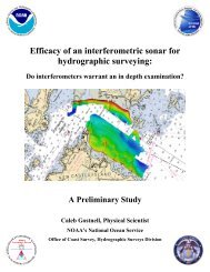
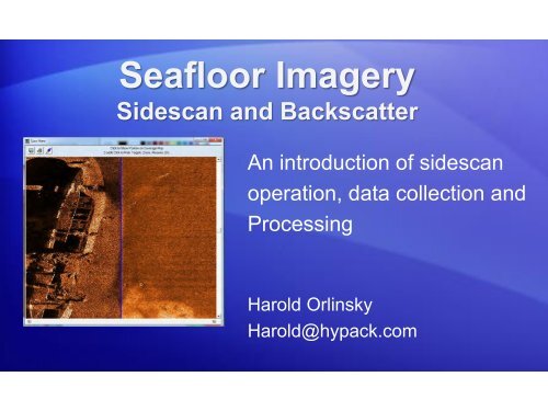
<strong>Seafloor</strong> <strong>Imagery</strong><br />
<strong>Sidescan</strong> <strong>and</strong> <strong>Backscatter</strong><br />
An introduction of sidescan<br />
operation, data collection <strong>and</strong><br />
Processing<br />
Harold Orlinsky<br />
Harold@hypack.com
Topics to cover<br />
• Introduction to the <strong>Sidescan</strong><br />
• <strong>Sidescan</strong> Theory<br />
• <strong>Sidescan</strong> Positioning<br />
• Resolution of systems (object detection)<br />
• <strong>Backscatter</strong><br />
• Data collection<br />
• <strong>Sidescan</strong> Mosaicking ( processing )<br />
• Data Interpretation<br />
• <strong>Sidescan</strong> data used for bottom classification<br />
That should keep us busy for the session.
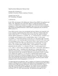
<strong>Sidescan</strong> systems – why use them<br />
• A sidescan sonar can be used<br />
for a wide variety of survey<br />
operations.<br />
• Search <strong>and</strong> recovery<br />
• Geological Identification<br />
• Pre / Post dredge surveys<br />
• Target verification <strong>and</strong><br />
location<br />
• It is also a useful tool for correlating<br />
• <strong>and</strong> verifying bathymetric data<br />
Shipwreck with shadow (in white)<br />
<strong>Sidescan</strong> data showing sediment change
<strong>Sidescan</strong> data for survey work<br />
A side scan:<br />
Will not give you depth information. Use a single beam<br />
or multibeam sonar for that.<br />
A side scan:<br />
Will give me information about targets on the seafloor,<br />
including their position <strong>and</strong> height above the bottom.<br />
Will give you real time information about the height of<br />
the fish above the bottom.<br />
Can be used for seafloor classification.<br />
Has a swath that is not depth dependent, like a<br />
multibeam.
<strong>Sidescan</strong> types<br />
<strong>Sidescan</strong> frequency can vary from 100kHz to over<br />
1Mhz. The higher the frequency, the better your<br />
resolution, but the shorter your range scale.<br />
Example: 100 Khz might be able to detect objects at 300meters,<br />
while a 900Khz will work to 45 meters<br />
<strong>Sidescan</strong> can be analog or digital. With an Analog<br />
system, an A/D is needed. See the Side Scan<br />
Hardware presentation for details.<br />
Some sidescan systems are multi-ping, <strong>and</strong> can be<br />
used while travelling at a high speed ( 10 to 12 kts )<br />
Single ping systems require you to survey at slow speeds to insure<br />
100% coverage.
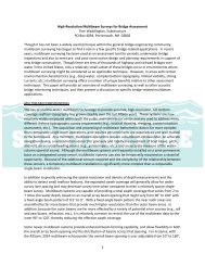
What you find with a <strong>Sidescan</strong> Record<br />
Shadow<br />
Water Column<br />
How the sonar sees the object:<br />
• Water Column - Provides information about towfish height.<br />
• Target - features off the seafloor will produce a shadow.<br />
• Bottom sediment - Signal will differ based upon return angle on incident<br />
<strong>and</strong> seabed absorption.
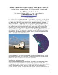
What to do with Side Scan data<br />
Mosaics <strong>and</strong> Targeting<br />
Mosaic:<br />
Survey lines can be merged together<br />
to provide a 2D representation of the<br />
seafloor <strong>and</strong> saved as a GeoTif file.<br />
Targeting: Capture <strong>and</strong> measure<br />
objects on seafloor. Targets can be<br />
saved to a file for reports<br />
Bottom Classification: GEOCODER<br />
Sample Mosaic of 5 survey lines<br />
Target report in HYSCAN
<strong>Sidescan</strong> Theory
Sonar system components<br />
• The sonar system (towfish) has a transmit <strong>and</strong> receive component<br />
taking the signal (digital) <strong>and</strong> sending to the acquisition computer for<br />
display <strong>and</strong> storage.<br />
• The echo distance is determined by time, similar to other sonar<br />
systems<br />
Display<br />
Transmitter<br />
/ receiver<br />
<strong>Sidescan</strong><br />
Signal<br />
Distance = time (round trip) x Sound Velocity<br />
2<br />
0 Time of pulse ------- <br />
Bottom<br />
echo<br />
Note the use of<br />
Sound Velocity. It is<br />
needed to compute<br />
the distance. The<br />
default of 1500 m/s<br />
will give an error
<strong>Sidescan</strong> operations - Positioning<br />
A sidescan, can be towed or fixed to a vessel.In either case, a swath of<br />
data is collected - port <strong>and</strong> starboard across the seafloor.<br />
During towed operations, the vessel is beyond the object when the sonar<br />
detects the echo. It is important to know the position of the sidescan,<br />
<strong>and</strong> use that for processing <strong>and</strong> targeting
<strong>Sidescan</strong> positioning<br />
Getting the position of the towfish is critical. Seeing<br />
an object but not knowing where it is, will not be very<br />
useful.<br />
•Cable out (layback)<br />
•Acoustic positioning system (USBL)<br />
•ROV (inertial systems on board)<br />
•Ship mounted (uses on board GPS with offsets)<br />
Which one is best Dependent of survey operations<br />
<strong>and</strong> water depth.
<strong>Sidescan</strong> positioning<br />
Where is the sonar located:<br />
At the vessel or towed system<br />
When at (on) the vessel, the position is set, but there are other problems<br />
When being towed, we lose confidence of the position of the targets<br />
Benefits<br />
Problems<br />
Towed Close to bottom Position (not<br />
Minimal motion<br />
accurate)<br />
Deep water work<br />
Hull Accurate position Shallow water work<br />
Mounted Won’t hit bottom (see next slide)<br />
Vessel motion will show
Operating a fixed mount (on survey vessel)<br />
RANGE SCALE<br />
Optimum Fish Height<br />
50 meter 4 – 10 meters<br />
75 meter 6 – 15 meters<br />
100 meter 8 – 20 meters<br />
A rule of thumb to get the best results:<br />
Use 8% to 20% of range scale for fish height<br />
•Why 8 – 20% or range scale This<br />
altitude will provide the best angle of<br />
incidence (reflection of an object) for a<br />
sonar return.<br />
Too shallow, high angle<br />
•When using a fixed mounted sidescan<br />
the image may degrade in water depths<br />
greater then 40 meters. The angle is too<br />
steep<br />
Too high, high angle
Towing a sidescan system<br />
Towing a sidescan allows for deep water operations.<br />
Some things to consider:<br />
1. Use of an A-frame or another method to deploy<br />
<strong>and</strong> recover the towfish<br />
2. Cable <strong>and</strong> winch system<br />
3. Position system – cable counter or Acoustic<br />
position<br />
4. Ship maneuverability<br />
Towfish deployment
<strong>Sidescan</strong> Resolution
Across track range resolution<br />
Why sonars work better at the outer ranges<br />
Distinguishing two independent objects can be referred to as<br />
the sonar resolution.<br />
If two objects are too close, they will appear as one on the sidescan<br />
record. Getting these objects further apart will show them as<br />
independent objects. How close can they be Half the pulse length.<br />
Example: A 500khz system has a pulse length of 1 cm.<br />
In practice, that won’t be seen, <strong>and</strong> cannot distinguish an object that<br />
close. We can approach this value further away from nadir.<br />
The footprint of sonar (arriving energy) is longer near nadir due to the<br />
angle of incident. Conversely, the further away, the more the bottom<br />
footprint approaches the pulse length.<br />
At the very far end of the signal, the best resolution would be obtained<br />
First<br />
return
Along track resolution<br />
why objects in the far field cannot be distinguished<br />
The resolution in the along track direction is dependent on the sonar<br />
Horizontal beam width.<br />
The image below represents what happens when targets in the far field<br />
are inside the angular resolution of the sonar. They become<br />
indistinguishable <strong>and</strong> look as a single object<br />
At the near field, these objects can be distinguished.<br />
Horizontal<br />
beam width<br />
First<br />
return
A combination effect – where object detection is ideal<br />
Looking at both the near field <strong>and</strong> far field constraints, as well as<br />
maximizing the best seen area, the sonar will work best in the region<br />
of the Optimal Zone of Operation (OZO)<br />
Targets is these areas<br />
might be missed or<br />
cannot be measured<br />
accurately<br />
Ideal location<br />
for targets
How to do a self check of object detection<br />
During survey operations, set the range scale of the sonar<br />
to your operating range.<br />
Run past a know object. A buoy block or s<strong>and</strong> waves will<br />
work<br />
Ensure that you can see the entire swath. If you can’t,<br />
shorten the range scale until you do.<br />
If you don’t see a known object,<br />
chances are you won’t find the<br />
unknown object.
<strong>Backscatter</strong>
<strong>Backscatter</strong><br />
How we see images on the seafloor.<br />
The sonar sends out energy, it gets deflected in all directions. The<br />
return signal can be from the surface <strong>and</strong> water column are<br />
reverberations, though typically low energy. The reverberations<br />
that come from the bottom are the ones we use to distinguish<br />
sediment types<br />
Surface<br />
Air bubbles<br />
fish<br />
Bottom features
<strong>Backscatter</strong><br />
Not all sound returning from the sonar is from direct echoes. On a flat<br />
bottom, the sound wave will reflect off the bottom <strong>and</strong> keep going.<br />
When there is some roughness on the bottom (<strong>and</strong> there usually is),<br />
the sound waves scatters on the return.<br />
The sound that comes back is detected, <strong>and</strong> can be used to<br />
distinguish different bottom types.
<strong>Sidescan</strong> data collection
Collecting sonar data is different than echosounder data<br />
Bold statement, but it is true.<br />
Survey operations will change when running a sidescan sonar<br />
• Vessel speed (slow is best – 5kts is typical)<br />
• Vessel h<strong>and</strong>ling (you can’t stop when towing a sidescan)<br />
• No turns during collection<br />
• line spacing is fixed (unlike multibeam collection)<br />
• Nadir area is obscured.<br />
• Visual display of waterfall gives immediate results<br />
• (sometimes that is good enough for folks)<br />
• <strong>Sidescan</strong> files are large, more storage needed<br />
But…. Even with all that, sidescan by itself or part of a survey operation<br />
provides very good results.
Data collection in HYPACK<br />
Two programs are running: HYPACK Survey (for GPS<br />
<strong>and</strong> positioning) <strong>and</strong> SIDE SCAN SURVEY (to h<strong>and</strong>le<br />
the sidescan system)<br />
Your computer<br />
HYPACK<br />
SURVEY<br />
SHARED<br />
MEMORY<br />
POSITION, HEADING,<br />
TIDE,, DEPTH<br />
SIDE SCAN<br />
SURVEY<br />
GPS<br />
Side Scan Sonar
Setting up a <strong>Sidescan</strong> Device<br />
• In HYPACK Hardware, add<br />
the driver to position your<br />
main vessel<br />
• GPS.DLL in this example.<br />
• Create a 2 nd mobile for your<br />
towfish position.<br />
• Named ‘Towed Array’ in<br />
this example.<br />
• Select a driver to position the<br />
towfish.<br />
• Towfish.DLL in this<br />
example.<br />
• Add the HYSWEEP.DLL to<br />
your towfish mobile.<br />
Setup menu for<br />
Towfish.DLL<br />
HYPACK hardware<br />
Device set-up has<br />
3 items in 2 mobile
Setting up a <strong>Sidescan</strong> Device<br />
In <strong>Sidescan</strong> Hardware:<br />
• Select position device:<br />
• HYPACK Navigation for<br />
vessel mount.<br />
• HYPACK Mobile<br />
for towfish mount.<br />
• Select <strong>Sidescan</strong> from the<br />
list of sensors.<br />
• Check Specific Sonar<br />
Identification (for<br />
processing data in<br />
Geocoder)
Connecting the sonar<br />
Sonar connections:<br />
There is serial (Imanegex) <strong>and</strong> USB (Tritech ,C-Max<br />
<strong>and</strong> the NI A/D board), but all the others are network<br />
based.<br />
Just know the port address <strong>and</strong> you’re set
Survey planning: 100% <strong>and</strong> 200% coverage<br />
100% coverage: At 100 meter range scale, line spacing would be set<br />
for 160 meters. This provides a 20 meter off-track error while<br />
surveying.<br />
200% coverage: This survey plan ensures that the bottom is covered<br />
twice by the <strong>Sidescan</strong>, covering the nadir region with the second<br />
line pass<br />
Line spacing<br />
160 meters<br />
Swath width<br />
200m<br />
Line spacing<br />
80 meters<br />
Note the overall swath<br />
width is twice the range<br />
scale
Data collection<br />
<strong>Sidescan</strong> survey<br />
Waterfall, Signal window,<br />
coverage map (real time<br />
mosaic) are all the tools you<br />
see during data collection
<strong>Sidescan</strong> TOOLS<br />
Many sidescan systems can be<br />
controlled inside SIDE SCAN<br />
SURVEY.<br />
In the Tools menu, select<br />
<strong>Sidescan</strong> Device Control.<br />
Settings for Range, Scale,<br />
Pinging, <strong>and</strong> certain gain controls<br />
can be sent to the sonar.<br />
During data collection, minimizing<br />
any gain changes or adjustments<br />
is best.<br />
A gain change will make the<br />
image look “darker”, but can be<br />
interpreted as a different bottom<br />
type.<br />
Know the survey area – <strong>and</strong> fix the<br />
range scale <strong>and</strong> gains before your<br />
start.<br />
Sample control boxes<br />
for different sonars
But… you still want to make sure the gains are set properly<br />
Display in waterfall with no adjustments. Notice the<br />
darken area near nadir, <strong>and</strong> the lighten area on the<br />
outer edge<br />
Raw Data: Gain = 0<br />
Auto TVG – Sigma = 7<br />
Use the gain controls to enhance the image, <strong>and</strong> to balance the signal
Maintaining a Proper Bottom Track is critical<br />
Why removing the bottom<br />
track isn’t a good idea:<br />
The bottom track will provides<br />
a visual display of how close<br />
the towfish is to the bottom.<br />
If you see something like<br />
this…Speed up or pull the<br />
cable in fast!
Capture <strong>and</strong> Measuring a contact:<br />
• To mark a target, double click in the waterfall.<br />
• To measure a target, select the up-arrow icon (4 th one in),<br />
<strong>and</strong> then double click. A target window will open<br />
Height of Contact (H) = L * A / R<br />
Three points along the<br />
image are needed<br />
altitude (A) , shadow length<br />
(L), total distance (R)
The target height may not be exact by two operators, due to the<br />
subjectiveness of shadow measurements<br />
Target Height Measurement<br />
Using the target window<br />
• Set Bar 1 to end of water column.<br />
• Set Bar 2 to target/shadow edge<br />
• Set Bar 3 to far end of shadow.<br />
• Use the signal display to assist in finding the target <strong>and</strong> shadow (look<br />
for low or weak signal following the target)<br />
Height above bottom<br />
Mark <strong>and</strong> save target.<br />
Target will be displayed in<br />
HYPACK survey
<strong>Sidescan</strong> mosaicking <strong>and</strong><br />
targeting
<strong>Sidescan</strong> Mosaic Processes<br />
Stage 1: Raw View<br />
Load raw sidescan data – HSX, HS2, XTF or LOG files<br />
Adjust bottom track, smooth heading <strong>and</strong> track line data.
<strong>Sidescan</strong> Mosaic Processes<br />
Stage 2: Scan View<br />
Full line can be viewed using the scroll bar.<br />
Adjust color, gain, TVG <strong>and</strong> display options (water column removal,<br />
display range of sonar image).<br />
Capture <strong>and</strong> measure targets (GeoTif <strong>and</strong> JPG images).
<strong>Sidescan</strong> Mosaic Processes<br />
Stage 3: Mosaic<br />
Create mosaics, export GeoTiff images. Apply image filters. Ability to use<br />
a Border file for mosaic creation in specific area.
Tiling of Mosaics<br />
Based on the<br />
resolution <strong>and</strong> the<br />
extents of your<br />
mosaic, HYSCAN<br />
may decide to subdivide<br />
your mosaic<br />
into several GeoTIF<br />
files.<br />
This allows you to<br />
mosaic a big area at<br />
a high resolution.<br />
It takes a little<br />
longer, but you’ll get<br />
the detail you need.
<strong>Sidescan</strong> Controls Adjustments<br />
Right-click on a side-scan image to get access to the<br />
<strong>Sidescan</strong> Controls window. ( short cut Shift+F9 ). <strong>Sidescan</strong><br />
controls <strong>and</strong> a sample of the data set appear in a single<br />
window.<br />
Select Color palate.<br />
Gray Scale, Gold, Copper, Rust, Pastel, Intensity, Custom. Invert Color scale<br />
Set Gains<br />
Manual or Auto TVG<br />
Remove Water Column<br />
Set Display Range<br />
Show Range lines<br />
RESET button sets<br />
gain thresholds to<br />
best fit value
<strong>Sidescan</strong> Controls Adjustments<br />
Colors Tab<br />
• Select color palate<br />
• Adjust overall brightness <strong>and</strong> contrast<br />
• Invert colors option
<strong>Sidescan</strong> Controls Adjustments<br />
Gains Tab<br />
• Set Gain <strong>and</strong> TVG<br />
• Port = Stbd.<br />
• Port <strong>and</strong> Stbd. Independent<br />
• Advanced Tab:<br />
• Apply Auto TVG <strong>and</strong> TVG curve (P1, P2 <strong>and</strong> P3)<br />
Show TVG Tab
Targeting<br />
Select Target (double<br />
left-click on feature)<br />
Target<br />
window<br />
opens<br />
Target screen displays contact. Use to take<br />
measurements, capture image <strong>and</strong> classify (new)<br />
In Stage 2, double click on any feature.<br />
Use sliders (top) to determine the 3 points along the target. Use the signal<br />
display to help.<br />
Click <strong>and</strong> drag to measure contact, capture JPG or TIF <strong>and</strong> enter any notes<br />
Save to a TGT file.
Targeting: Example
Measuring a contact:<br />
Three points along the image are needed<br />
altitude (A) , shadow length (L), total distance (R)<br />
Height of Contact (H) = L * A / R<br />
Each target will have a shadow; use the tools in <strong>Sidescan</strong> Survey or<br />
HYSCAN to measure contact
Target Viewer <strong>and</strong> Classification<br />
Use the target viewer to examine all contacts.<br />
Arrow keys to scroll through the list of targets.<br />
Data fields in the target viewer are editable for any changes or updates.<br />
Report can be saved to a RTF file<br />
TargetViewer program can run without a HYPACK key
Target Classification Database<br />
Select Tools – Target Classification<br />
Database to open/revise database<br />
Creating the Database<br />
Target database can be made<br />
of any target image. User<br />
can add a confidence level<br />
<strong>and</strong> notes to each target<br />
Using the Database in Target Viewer<br />
In Target Viewer, select from classification drop<br />
down the targetID. Use the To open the<br />
comparison window<br />
Target classification<br />
comparison<br />
Classification<br />
database<br />
Target Viewer
Resolution Calculator<br />
Determine the optimal mosaic<br />
resolution based on your<br />
sonar's characteristics<br />
• Don't waste time <strong>and</strong> space<br />
on heavily-interpolated<br />
imagery<br />
• Calculate Along-track <strong>and</strong><br />
across-track resolution<br />
• Load & Save sonar profiles<br />
across HYPACK projects<br />
• When closed, the best<br />
resolution is applied to the<br />
mosaic setup
Mosaic Filter options<br />
AVERAGE:<br />
Smoothes the mosaic<br />
by setting each pixel<br />
to the average of the<br />
3x3 pixel<br />
neighborhood<br />
SHARPEN:<br />
Sharpens the mosaic<br />
by enhancing pixel<br />
contrast relative to a<br />
3x3 pixel<br />
neighborhood<br />
MEDIAN:<br />
Smoothes the mosaic<br />
while preserving<br />
edges by setting each<br />
pixel to the 3x3 media<br />
value.
Using Coverage Map to manage targets<br />
Blue bounding box = previous<br />
line Red bounding box =<br />
current line<br />
Note the difference in<br />
position (approx 6 meters)<br />
when viewed in Scan View.<br />
Possible cause could be<br />
improper layback setting.<br />
• When a target is taken, a mark is generated on the coverage<br />
map. Use this feature to verify location or to confirm target
Target Viewer<br />
• Used to view side scan targets marked in HYSCAN.<br />
• Can be run as a st<strong>and</strong> alone program without a dongle.<br />
• Can save target info to RTF (Rich Text Format) that can be read into Microsoft Word.
<strong>Sidescan</strong> Interpretation
Take a look at this image. What is it
The Shadow Effect<br />
Imaging the seafloor from above will cast a shadow of the object. Sometimes<br />
the shadow can give you more information that just the data on the seafloor
<strong>Sidescan</strong> interpretation<br />
• Besides shadows, the feature<br />
itself can give some indication<br />
of the object. Colors ( light <strong>and</strong><br />
dark ) can be inferred as<br />
different bottom types. In this<br />
example, we see an area of<br />
light <strong>and</strong> dark.<br />
• Without knowing anything else,<br />
we can say it is a different<br />
bottom type.<br />
• With ancillary information,<br />
depth data in this example, we<br />
can say it is a hard bottom<br />
(dark grey - deep), soft bottom<br />
(light grey-shallow).
Proving the chart is wrong<br />
On the chart, we<br />
see the outline<br />
for a dock.<br />
The sidescan is<br />
showing the<br />
piles 200 feet<br />
south.<br />
A position error<br />
Nope!
A floating dock
<strong>Sidescan</strong> for bottom<br />
classification<br />
(Geocoder)
GEOCODER<br />
• Developed by Dr. Luciano Fonseca, formerly of UNH-CCOM<br />
• Creates mosaics from:<br />
– Side Scan<br />
– Multibeam Average <strong>Backscatter</strong><br />
– Multibeam Snippets<br />
• Advanced <strong>Backscatter</strong><br />
Correction Algorithms<br />
• Bottom Classification using<br />
Angular Response Analysis<br />
60
GEOCODER Data Flow<br />
Side Scan Data<br />
Fix Bottom Detection<br />
SIDE SCAN<br />
SURVEY<br />
HSX<br />
SIDE SCAN<br />
MOSAIC<br />
HS2<br />
Multibeam Average <strong>Backscatter</strong> & Snippet Data<br />
GEOCODER<br />
HYSWEEP<br />
SURVEY<br />
HSX<br />
MBMAX<br />
HS2<br />
81X/7K/R2S<br />
GSF<br />
Bathymetric Model (optional)<br />
MTX or XYZ<br />
81X/7K/R2S<br />
TIF<br />
61
Input Data Files<br />
• Average <strong>Backscatter</strong><br />
(HS2/GSF)<br />
• Snippets (HS2/GSF)<br />
• Side Scan (HSX/HS2)<br />
• Side Scan <strong>and</strong> DTM<br />
• Side Scan: (HSX/HS2)<br />
• DTM (XYZ-Gridded, MTX)<br />
Bringing in a DTM allows you to enhance your mosaic with angle varied<br />
gain algorithms.<br />
62
Remosaicing<br />
Users can remosaic entire lines or sections of lines.<br />
Normally used to change the overlap option.
Bathymetric Corrections<br />
Load a bathymetric model from<br />
MTX or XYZ to apply:<br />
• correction for actual angle of<br />
incidence for all data types.<br />
• improved area correction<br />
• improved slant-range<br />
correction for side scan data.<br />
• DTM must be a gridded XYZ or a<br />
MTX file.
Bottom Classification: Extracting the Beam Pattern<br />
• Each sonar can have its own particular<br />
faults that influence the acoustic beam<br />
pattern.<br />
• In GEOCODER, users can make<br />
adjustments based on the sonar’s beam<br />
pattern.<br />
1. Isolate a short swath over a flat, boring<br />
bottom.<br />
2. Use the ‘Extract Beam Pattern’ menu item to<br />
determine the adjustment for the sonar.<br />
3. Save the resulting beam pattern adjustment<br />
to a file.<br />
4. After extracting the beam pattern, or reading a<br />
previously extracted beam pattern file, your<br />
data will be automatically adjusted.<br />
AVI
Bottom Classification: Angular Response Analysis<br />
• Used to determine bottom classification across a swath.<br />
• Matches acoustic response to known bottom types.<br />
1. Create the mosaic.<br />
2. Calculate the ARA for the mosaic.<br />
3. Select a swath from the mosaic screen.<br />
4. Run the ARA – Patch ARA routine.<br />
AVI 1<br />
AVI 2<br />
Patch ARA Analysis Window<br />
Color-coded ARA<br />
Selecting a swath for ARA Analysis<br />
66
Output ARA results to DXF<br />
Export ARA results to a DXF contour map<br />
• You must enable the ‘Formal Inversion.<br />
• When completed, click the Save DXF menu item at the bottom.
A lot to see in an hour (or so).<br />
There is good reference material<br />
around, especially from the sonar<br />
manufactures<br />
- <strong>and</strong> most are here today<br />
Questions