Robust UAV Search for Environments with Imprecise Probability Maps

analyzed to determine the impact of uncertainty measures
on N. The analytical properties are presented based on
expected value and variance objectives. These results clearly
show a diminishing returns effect with additional looks,
which is generally modeled in classical search theory (see
Ref. [15]) with the decaying exponential detection function.
Section V demonstrates the benefits of the approach with
several numerical simulations.
12
10
8
6
b = 100, c = 50
II. SEARCH PROBLEM AND BETA DISTRIBUTIONS
Search problems are generally posed by discretizing the
environment in an grid of cells over a 2-dimensional space
indexed by (i, j) ∈ (I,J). Each cell is available to contain a
target, but this knowledge is not known prior to the search. It
is therefore estimated with a target existence probability, P ij .
Also known as a target occupancy probability (e.g., [11]),
the target existence probability is the probability that the
particular cell contains an active target. The complement of
this probability, 1 − P ij , denotes the probability that a cell
does not contain a target. If the target is known to exist in
a cell, then the precise probability of target existence in the
cell is P ij =1. Alternatively, if the target does not exist,
P ij =0.
Given a limited number of UAVs to accomplish the search,
typical allocation problems ([11], [16]) assign the vehicles to
the cells that have the highest probability of target existence.
This is a reasonable objective if the prior probabilities are
known precisely; however, this will be difficult to achieve in
real-life operations. In general, the prior probabilities come
from intelligence and previous observations, and cannot be
treated as completely certain. Earlier results indicating the
effect of uncertainty in resource allocation problems were
presented in Refs. [4], [5], and showed that performance
can be lost if uncertainty is not properly accounted for in
resource allocation problems. As such, a practical framework
needs to be developed that appropriately takes into account
the uncertainty in this information for search operations.
Various approaches have been developed in the literature
to describe the uncertainty in a probability P ij .The
approaches in [6], [7] have considered interval probability
descriptions where the probability is within a given range of
values (P ij ∈ [P min ,P max ]). This formulation is appealing
because of its simplicity, but there are difficulties in propagating
this range of probabilities in a Bayesian framework.
An alternative method of describing the uncertainty in the
probability is to use scenarios (e.g., [13]), where each
of the scenarios consists of a realization of the different
prior probabilities for each cell. However, these approaches
may require a large number of scenarios before the entire
uncertain probability is accurately modeled, and can be
computationally intensive.
The uncertainty in the probability can also be described
using Beta distributions (e.g., [8], [10]). The Beta distribution
is a very general distribution that treats P ij as a random
variable, and has various appealing features: 1) The support
of the Beta distribution, the random variable P ij ,isonthe
open interval (0, 1); 2) The Beta distribution is conjugate
4
2
b = 10, c = 5 b = 5, c =
2.5
0
0 0.2 0.4 0.6 0.8 1
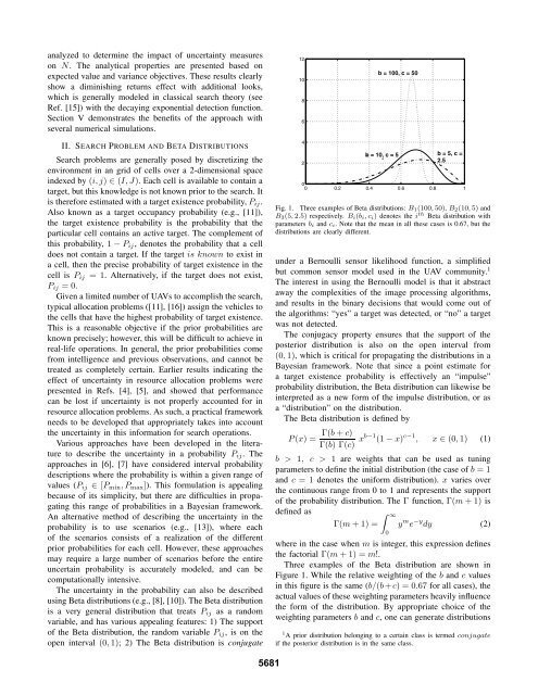
Fig. 1. Three examples of Beta distributions: B 1 (100, 50), B 2 (10, 5) and
B 3 (5, 2.5) respectively. B i (b i ,c i ) denotes the i th Beta distribution with
parameters b i and c i . Note that the mean in all these cases is 0.67, but the
distributions are clearly different.
under a Bernoulli sensor likelihood function, a simplified
but common sensor model used in the UAV community. 1
The interest in using the Bernoulli model is that it abstract
away the complexities of the image processing algorithms,
and results in the binary decisions that would come out of
the algorithms: “yes” a target was detected, or “no” a target
was not detected.
The conjugacy property ensures that the support of the
posterior distribution is also on the open interval from
(0, 1), which is critical for propagating the distributions in a
Bayesian framework. Note that since a point estimate for
a target existence probability is effectively an “impulse”
probability distribution, the Beta distribution can likewise be
interpreted as a new form of the impulse distribution, or as
a “distribution” on the distribution.
The Beta distribution is defined by
Γ(b + c)
P (x) =
Γ(b) Γ(c) xb−1 (1 − x) c−1 , x ∈ (0, 1) (1)
b > 1, c > 1 are weights that can be used as tuning
parameters to define the initial distribution (the case of b =1
and c =1denotes the uniform distribution). x varies over
the continuous range from 0 to 1 and represents the support
of the probability distribution. The Γ function, Γ(m +1) is
defined as
∫ ∞
Γ(m +1)= y m e −y dy (2)
where in the case when m is integer, this expression defines
the factorial Γ(m +1)=m!.
Three examples of the Beta distribution are shown in
Figure 1. While the relative weighting of the b and c values
in this figure is the same (b/(b + c) =0.67 for all cases), the
actual values of these weighting parameters heavily influence
the form of the distribution. By appropriate choice of the
weighting parameters b and c, one can generate distributions
1 A prior distribution belonging to a certain class is termed conjugate
if the posterior distribution is in the same class.
0
5681