Robust UAV Search for Environments with Imprecise Probability Maps
Robust UAV Search for Environments with Imprecise Probability Maps
Robust UAV Search for Environments with Imprecise Probability Maps

You also want an ePaper? Increase the reach of your titles
YUMPU automatically turns print PDFs into web optimized ePapers that Google loves.
0.65 0.7 0.75 0.8 0.85 0.9 0.95 1<br />
3<br />
ξ = 0.80 ξ = 0.98<br />
TABLE I<br />
NUMBER OF LOOKS FOR DIFFERENT η: b =1, c =1, ξ =0.85<br />
Log 10<br />
(N)<br />
2.5<br />
2<br />
1.5<br />
1<br />
η µ N<br />
0.70 0.01 2.7<br />
0.75 0.01 5.1<br />
0.80 0.01 12.2<br />
0.84 0.01 71.1<br />
0.5<br />
0<br />
Fig. 3. The logarithm of the number of looks is plotted against α <strong>for</strong> two<br />
distinct sensor errors. Note that as α −→ ξ, the number of looks increases<br />
very rapidly, and there is a diminishing returns behavior.<br />
accuracy ξ. This means that there is a fundamental limitation<br />
to the expected value of the posterior subject to the sensor<br />
accuracy: the chosen threshold α cannot exceed the accuracy<br />
of the sensor.<br />
Furthermore, the number of looks can become increasingly<br />
large as the expected value of the posterior density is<br />
increased. In the case that α → ξ the righthand side of<br />
Eq. (11) tends to infinity (see examples in Figure 3). This<br />
property underscores the “diminishing returns” behavior of<br />
this model. As α is increased, the number of looks rapidly<br />
increases (note that the y-axis is a logarithmic scale). One<br />
important observation from the figure is that, <strong>for</strong> lower sensor<br />
accuracies, there is a fundamental limit to the expected value<br />
of the posterior density. Further, if this value is chosen to be<br />
close to the sensor accuracy, the number of looks can become<br />
prohibitively large.<br />
Remark 3 (Result B) The two parameters η and µ have a<br />
significant impact on the number of looks that are required<br />
to achieve a certain confidence in the target presence. There<br />
is an intrinsic interplay between the parameters µ and η in<br />
finding the optimal arrangement to suit a mission, and this<br />
will be ultimately the responsibility of the mission designer.<br />
Care must also be taken in choosing the parameters η, µ to<br />
ensure that when the cubic equation is solved, that N is real<br />
and positive.<br />
Table I shows two cases <strong>for</strong> the uni<strong>for</strong>m distribution (b =<br />
1, c=1), <strong>with</strong> a sensor accuracy of ξ =0.85. TableIshows<br />
the effect of varying η <strong>for</strong> constant µ. As shown in Figure 3,<br />
when η ≈ ξ, the number of looks increases significantly <strong>for</strong><br />
a marginal increase in the threshold.<br />
V. NUMERICAL RESULTS AND DISCUSSION<br />
This section presents some numerical results that show the<br />
effectiveness of the expected value approach of Section IV<br />
and compares it to heuristics assuming nominal in<strong>for</strong>mation.<br />
In this analysis 4 targets are present in the environment;<br />
the imprecise prior in<strong>for</strong>mation indicates that there is only a<br />
50% chance of the targets actually existing (this is the point<br />
α<br />
estimate, and implies the total number of targets is unknown).<br />
The priors are described by Beta distributions, where the<br />
(b, c) values are next to the target number in Table II. Note<br />
that the cells have different (b, c) values, and will thus require<br />
a different number of looks to exceed the threshold. The<br />
purpose of the mission is to determine how many targets<br />
actually exist by assigning the <strong>UAV</strong> as indicated in Figure 4,<br />
and taking the predicted number of looks in each cell. The<br />
total number of looks will allow the mission designer to<br />
predict the length of the mission. In the case of the analytical<br />
result, a total Time on Target (ToT) <strong>for</strong> the i th target (T i )is<br />
calculated based on the prior in<strong>for</strong>mation, using Eq. 11. The<br />
thresholds that are obtained <strong>with</strong> these number of looks are<br />
calculated in 1000 Monte Carlo simulations, and compared<br />
in Table II.<br />
3<br />
2.5<br />
2<br />
1.5<br />
1<br />
0.5<br />
<strong>UAV</strong> Traj<br />
Target 1<br />
P=0.5<br />
Target 4<br />
P=0.5<br />
Target 3<br />
P=0.5<br />
Target 2<br />
P=0.5<br />
0<br />
0 0.5 1 1.5 2 2.5 3<br />
Fig. 4. Visualization of the environment discretized in 9 cells. 4 targets<br />
are present in the environment, and the prior probability <strong>for</strong> each is 0.5.<br />
The <strong>UAV</strong> has a unique number of looks that it can place on each target.<br />
The heuristics used specify that looking in a cell <strong>for</strong> a<br />
predefined amount of time will allow the operator to exceed<br />
the threshold <strong>for</strong> which the target is unambiguously declared<br />
absent or present in the cell. Some of these heuristics have<br />
been used in the literature to model the need to look in a<br />
cell a sufficient number of times to increase the threshold in<br />
a cell ( [9]). Three heuristics are compared to the analytical<br />
expressions obtained in this paper. In the first heuristic, the<br />
maximum amount of time (T A =max i (T i ), ∀i) istakenin<br />
each cell; in the second heuristic, the minimum time (T B =<br />
min i (T i ), ∀i) is taken in each cell; in the third heuristic,<br />
the average length of time (T C = ¯T i , ∀i) is taken in each<br />
cell. The key point in this experiment is that the individual<br />
5684