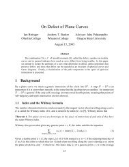
Irreducible Plane Curves 1 Reducibility of Curves

Irreducible Plane Curves
Jason E. Durham
Oregon State University
Corvallis, Oregon
durhamj@ucs.orst.edu
August 24, 1999
Abstract
Progress in the classication of plane curves in the last ve years has
centered largely around the work of Arnold, Vassiliev, and Aicardi. The
classical index theorem of H. Whitney (1937) classies curves by index,
up to isotopy. Arnold has recently proposed new curve invariants + (J ,
J , , and St) with the aim of nding classications of curves with the same
index, up to ambient dieomorphisms of the plane and reparametrizations
of the curve.
Since these new invariants still do not uniquely determine curves, new
ways of classifying curves up to dieomorphisms have been sought. A
certain class of curves (so called \reducible" curves) appears to be classi-
able by direct consideration via relatively simple combinatorial methods
involving combinations of irreducible curves. This shifts the focus to the
classication of the irreducible curves, whose characterization appears to
be simplied by association with certain types of planar graphs.
1 Reducibility of Curves
Throughout this article, \ambient dieomorphisms of the plane and reparametrizations
of the curve" may be shortened to \dieomorphisms." \Distinct" is
short for \distinct up to dieomorphisms."
Denition 1.1. An immersion of a circle into the plane is a smooth mapping
of a circle into the plane : S 1 ! R 2 whose derivative never vanishes.
Denition 1.2. A double point (respectively, n-point) on an immersion of a
circle into the plane is a point that is the image of exactly two (respectively,
n) points on S 1 under . The term crossing will be used interchangeably with
double point.
Under the guidance of Professor Juha Pohjanpelto of Oregon State University
35

Figure 1: An inverted sum of two curves.
Denition 1.3. A curve shall be dened as an immersion of a circle into the
plane that contains no self-tangencies and where every n-point is a double point.
Denition 1.4. A strand of a curve is a segment of the curve that runs from
one crossing to another with no crossings in between. For consistency we also
consider the whole image of S 1 to be a strand even though it has no crossings.
Note 1. Let Str denote the number of strands on a curve , and R denote the
number of regions into which the curve divides the plane. For every n-crossing
curve besides S 1 , Str =2n. Recall that Str S 1 is dened to be 1.
Denition 1.5. The inverted sum between two strands of two curves is the
new curve shown in Figure 1.
Denition 1.6. A reduction cut at a crossing on a curve is a surgery and subsequent
smoothing that separates the image of the curve into two disjoint, welldened
curves (see Figure 2).
Note that the reduction cut has the opposite eect of the inverted sum
procedure (see Figure 2).
Denition 1.7. A reduction point is a double point on a curve at which a
reduction cut can be performed.
Denition 1.8. A curve is said to be reducible if it has a reduction point. That
is, there exists some crossing on the curve that divides the image of the curve
into two curves with no other points in common. A curve iscompletely reducible
36

REDUCTION CUT
INVERTED SUM
Figure 2: Opposite procedures.
if every crossing on the curve is a reduction point. A curve ispartially reducible
if it has a reduction point and also has a crossing that is not a reduction point.
A curve isirreducible if it has no reduction points.
Figure 3 shows a list of the irreducible curves with ve orfewer crossings.
The numbers associated with the curves will be used later to aid in referring to
them.
Proposition 1.1. The inverted sum of two immersions always has a reduction
point | the double point created by the inverted sum procedure.
Proof. Evident, by doing the reduction cut procedure corresponding to whatever
inverted sum procedure yielded the inverted sum.
Note 2. Let 1 and 2 be two arbitrary curves. After taking any inverted sum
of 1 and 2 ,any crossings that had been reduction points on 1 or 2 will be
reduction points on the curve resulting from the inverted sum, and any crossings
on 1 and 2 that had not been reduction points will not be reduction points
on the resulting curve. The new crossing formed by the inverted sum procedure
will by Proposition 1.1 be a reduction point. Similarly, performing a reduction
cut procedure at a crossing on a curve cannot change the status of any ofthe
other double points with respect to reducibility.
Proposition 1.2. Any completely reducible curve can be expressed as a sequence
of inverted sums of standard circles. Conversely, every sequence ofinverted
sums of standard circles yields a completely reducible curve.
Proof. Consider an arbitrary completely reducible curve with n crossings (hence
n reduction points). Perform a reduction cut at every crossing; this yields a set
of n + 1 circles. Now itis clear that performing the inverted sums that undo
the reduction cuts will produce the original curve.
37

0.1
3.1 3.2
4.1 4.2 5.1
5.2 5.3 5.4
5.5 5.6
Figure 3: The irreducible curves with n 5 double points. The number to the
left of the decimal indicates the number of crossings. The number to the right
is just an arbitrary indexing number.
38

For the converse, we proceed by induction: taking one inverted sum between
two standard circles can only result in two possible curves, both of which have
one crossing and are completely reducible by Proposition 1.1 (see Figure 5).
It follows directly from Note 2 that an inverted sum of any two completely
reducible curves must yield a completely reducible curve. By induction, every
sequence of inverted sums of standard circles must produce a completely
reducible curve.
Corollary 1.3. Any sequence of inverted sums of completely reducible curves
must result in a completely reducible curve.
Proof. Evident, via the theorem.
Proposition 1.4. Every reducible curve can be expressed asasequence ofinverted
sums of irreducible curves; there isnosequence of inverted sums of curves
that yields an irreducible curve.
Proof. Consider an n-crossing reducible curve with m reduction points. Perform
the reduction cut at every reduction point; this must yield m + 1 curves, and
by Note 2, no crossings on any of these m + 1 curves can be reduction points,
so each of the curves must be irreducible. Now it is clear that performing the
inverted sums that undo the reduction cuts we made before will produce the
original curve.
Consider an arbitrary sequence of inverted sums of curves. By Proposition
1.1 and Note 2, the resulting curve must have a reduction point, hence it
is reducible.
Proposition 1.5. Any partially reducible curve can be expressed asasequence
of inverted sums of curves where at least one of the factor curves is not completely
reducible. Conversely, every sequence ofinverted sums of curves where
at least one of the factor curves is not completely reducible yields a partially
reducible curve.
Proof. Consider an arbitrary partially reducible curve. Since it has a reduction
point it can be reduced into two curves, so it is clear that it is the result of some
inverted sum of curves. The question is whether it is necessary that one of the
factor curves not be completely reducible. Corollary 1.3 shows that it is.
For the converse, consider an arbitrary sequence of inverted sums of curves
where at least one of the factor curves is not completely reducible. By Proposition
1.4, this sequence of sums cannot yield an irreducible curve. Note 2 shows
additionally that the resulting curve cannot be completely reducible. The resulting
curve is therefore partially reducible.
2 Irreducible Curves as Building Blocks
We would like to be able to write every reducible curve as a set of n irreducible
curves together with n , 1 pairs of strands from those curves that indicate
39

Figure 4: The decomposition of a reducible curve.
which inverted sums would need to be taken to reconstruct the reducible curve
in question. Figure 4 shows a complicated reducible curve reduced down to
its constituent irreducible curves and recipe of connected sums. But is this
decomposition unique That is, is there any other set of irreducible curves or
recipe of inverted sums that would yield the same reducible curve The following
theorem shows there is not.
Theorem 2.1. Upon decomposition, every reducible curve gives rise to a unique
set of irreducible curves together with a unique set of inverted sums among those
curves that yields the curve in question.
Proof. Consider an arbitrary reducible curve with m reduction points. Recall
from Note 2 that performing the reduction cut at these reduction points doesn't
change the status of any ofthe other double points with respect to reducibility.
Thus after performing the m possible reduction cuts, we will have m +1
irreducible curves, as well as a set of m reduction cuts to repair with m specic
inverted sums. Since these reduction cuts can only be made in one way, the irreducible
factor curves are uniquely determined; the inverted sums are uniquely
determined as the reverse procedures of the reduction cuts. This proves the
theorem.
Assuming the above theorems, if one were to know all the irreducible curves
with n

Figure 5: All the distinct inverted sums of two copies of S 1 yields all the distinct
curves with one double point.
n k crossings comes down to more basic combinatorics. One would try to nd
the distinct combinations of inverted sums involving irreducible curves with n<
k crossings; this should produce all the reducible curves with n k crossings.
As a simple example, we can derive all the 1-crossing curves by taking all the
possible inverted sums of two copies of S 1 . Since each circle has only one strand,
there are only two distinct ways of taking their inverted sum (see Figure 5).
Denition 2.1. A reducible curve is n-reducible if it has n reduction points.
Note that such a curve has exactly n + 1 irreducible factor curves.
Denition 2.2. The inverted sum set (ISS) of two irreducible curves (denoted
ISS( 1 ; 2 )) is the set of all distinct curves that can result from any inverted
sum between 1 and 2 . For example, Figure 5 shows ISS(S 1 ;S 1 ).
Proposition 2.2. We can put an upper bound on the cardinality of ISS( 1 ; 2 ),
where 1 is an m-crossing curve and 2 is an n-crossing curve, by
Card(ISS( 1 ; 2 )) Str 1 Str 2 (m + n +3)
and, provided that neither 1 nor 2 is S 1 ,
Card(ISS( 1 ; 2 )) 4mn(m + n +3)
Proof. The formula derives easily by considering the possible cases: rst consider
the case where the two curves are unnested (i.e., one in the left half-plane
and the other in the right half-plane). The worst case scenario would be for
neither curve to have any kind of symmetry, forcing every strand to be considered
individually. Then every unique pair of strands, one from 1 and the
other from 2 , could have an associated inverted sum between the two curves
and every one of those inverted sums could result in a distinct curve. So far
this gives Str 1 Str 2 as an upper bound. Now consider the cases where one
curve is nested inside one of the bounded regions of the plane delineated by the
other. The worst case again gives Str 1 Str 2 as the upper bound. There are an
additional n + 1 cases for 1 nested in 2 , and m + 1 cases for 2 nested in 1 .
The total cases are (n +1)+(m +1)+1=m + n + 3, which is exhaustive.
41

Remark 2.1. This upper bound is very generous and there are probably very
simple considerations that could be taken into account to make it tighter. For
example, Card(ISS(S 1 ; 3:1)), where 3:1 is the three-crossing trefoil curve, is
given an upper bound of 36 by the formula, when the actual number is only
5. It is nice, however, to be able to condently give an upper bound on the
number of 1-reducible 6-crossing curves. The only inverted sum sets that yield
such curves are sets where one curve has one crossing and the other has ve,
or where both curves have three crossings (there are no 2-crossing irreducible
curves to pair with any of the 4-crossing irreducibles). The above formula gives
1452 as the maximum possible numberofsuch curves. Similar methods could be
applied to nd upper bounds for 2-reducible curves and beyond, which, together
with an upper bound on the number of irreducibles, would yield upper bounds
on the total number of curves with a given number of crossings.
Note how, in Figure 5, the symmetry of the two curves (in this case, the
\symmetry" is the fact that the two factor curves are identical) has made one
of the possible three cases equivalent | the inverted sum with circle A inside
of circle B and the inverted sum with circle B inside of circle A are equivalent
cases. In general, any symmetry within either of the curves involved or between
the two curves seems to reduce the number of distinct inverted sums. The fact
that many curves have several symmetries is another reason the upper bound
given above is so generous.
When we can identify how many symmetrically distinct regions irreducible
curves have and how many symmetrically distinct strands border each region
(this seems very easy, at least for curves with low numbers of crossings), we can
give an exact number for the cardinality ofany ISS involving these curves.
Notation. For any irreducible curve , let U be the unbounded region of the
plane delineated by and label the rest of the symmetrically distinct regions
A; B; C; . Let u be the number of symmetrically distinct strands bordering
U, and a; b; c be the number of symmetrically distinct strands bordering
A; B; C; , respectively.
Proposition 2.3. The cardinality of ISS( 1 ; 2 ) is given by
Card(ISS( 1 ; 2 )) = u 1 u 2 + u 1 (a 2 + b 2 + + j 2 )+u 2 (a 1 + b 1 + + k 1 )
if 1 and 2 are dierent curves, and
Card(ISS( 1 ; 2 )) = (u 1 2 + u 1 )=2+u 1 (a 2 + b 2 + + j 2 )
if the two curves are identical.
Proof. This proof follows the proof of Proposition 2.2, reducing the number
of regions and strands to the symmetrically distinct ones. The arguments are
analogous except where noted. The u 1 u 2 term derives from the case where the
two curves are unnested. The u 1 (a 2 + b 2 + + j 2 ) term accounts for the cases
where 1 is nested in 2 , and the u 2 (a 1 + b 1 + + k 1 ) term accounts for the
42

cases where 2 is nested in 1 . When 1 and 2 are identical curves, the cases
where 1 is nested in 2 are not distinct from the cases where 2 is nested in
1 , so we drop the u 2 (a 1 + b 1 + + k 1 ) term. When they are unnested the
redundant combinations of distinct strands end up eliminating half of the cases
where two dierent strands are involved, giving the (u 12 + u 1 )=2 term.
For example, to verify that Card(ISS(S 1 ;S 1 )) = 2, label the region inside
the rst circle A 1 , the region inside the second circle A 2 . Then u 1 = u 2 = a 1 =
a 2 =1,sowehave
Card(ISS(S 1 ;S 1 ))=1+1=2
It is helpful to have a listing of the values of u; a; b; c; for the irreducible
curves. These are the values for the irreducible curves up to ve crossings.
curve u a b c d e
0.1 1 1 - - - -
3.1 1 2 1 - - -
3.2 1 2 1 - - -
4.1 2 3 2 2 1 -
4.2 1 2 2 1 - -
5.1 1 2 1 - - -
5.2 1 3 1 1 - -
5.3 1 2 2 1 - -
5.4 2 4 2 2 1 1
5.5 1 4 2 2 2 1
5.6 2 3 2 2 1 -
With this table we can easily compute, for example,
Card(ISS(5:5; 5:6))=2+1(3+2+2+1)+2(4+2+2+2+1)=32
As noted above, the upper bound formula for the ISS gives 1452 as an upper
bound on the number of 1-reducible 6-crossing curves. Now we can compute
the exact number:
Card(ISS(3:1; 3:1)) = 4
Card(ISS(3:1; 3:2)) = 7
Card(ISS(3:2; 3:2)) = 4
Card(ISS(5:1; 0:1)) = 5
Card(ISS(5:2; 0:1)) = 7
43

Card(ISS(5:3; 0:1)) = 7
Card(ISS(5:4; 0:1))=14
Card(ISS(5:5; 0:1))=13
Card(ISS(5:6; 0:1))=12
(T otal = 73)
For the determination of the set of distinct inverted sums of curves with
low numbers of crossings using few inverted sums, the combinatorics involved in
constructing the reducible curves is simple, but for higher numbers of crossings
or more inverted sums the combinatorics problem is dicult, as it is at least
as hard as the problem of nding the distinct trees with n vertices. In [2],
F. Aicardi discusses combinatorial structures for completely reducible curves in
terms of trees; it appears that the combinatorics for the completely reducible
curves can be easily adapted for partially reducible curves. Such a modication
of Aicardi's theory seems a promising direction for future research.
3 Finding the Irreducibles
So we see that in some sense the irreducible curves are the building blocks for
the space of plane curves, for if we know them we can construct the other curves
by combinatorial methods based on the nesting of the factor irreducible curves
and the choice of which of their strands to join with the inverted sum. From here
the most imperative problem seems to be to nd, characterize, and classify the
irreducible curves. The most promising approach so far has been to associate
a certain type of planar graph with irreducible curves and then to nd all the
distinct graphs of that type.
Denition 3.1. A closed planar graph is a graph in which none of the edges
intersect and where removing any edge would decrease the number of regions
formed by the graph by one.
It will become clear later that every irreducible curve has a corresponding
closed planar graph that is unique to that curve. The nature of that correspondence
is well known; the following explanation and claims are based on
information from pp. 51-55 of [1]. (The validity of the following method seems
intuitively correct and has so far been very successful in deriving irreducible
curves, but proving the legitimacy of the method rigorously would have taken
more time than was available | perhaps future work could be done to ll in
the details, assuming similar work has not already been carried out.)
Every n-crossing curve divides the plane into n +2 regions that are 2-
colorable. That is, the regions can be colored so that no like colored regions are
adjacent (see Figure 6). (To readers of [3] a new proof of this fact is evident
using Arnold's perestroikas on the K i curves, by showing that the moves J + ,
J , , and St do not change the colorability.) We call a region bounded by a curve
44

Figure 6: A 2-coloration of an irreducible curve.
Figure 7: The closed planar graph associated with an 6-crossing irreducible
curve.
an exterior region if it must receive the same color as the unbounded region in
a 2-coloration; we call a region interior if it is not exterior.
A closed planar graph associated with an irreducible curve is constructed
as follows. Place a vertex inside each interior region and then place edges that
connect the vertices through the crossings without letting the edges cross, as
in Figure 7. Notice that every crossing is traversed by exactly one edge, and
that every region of the graph encloses exactly one exterior region of the curve
(with the exception of the unbounded region). It is not dicult to see that an
irreducible a curve can always be constructed uniquely from its graph, and that
every irreducible curve has a unique associated closed planar graph.
This representation of irreducible curves as closed planar graphs reduces the
problem of nding all the irreducible curves to an apparently simpler combinatorics
problem: nd all the distinct closed planar graphs with certain re-
45

strictions. These restrictions fall out easily from basic properties of irreducible
curves. In the following, V shall denote the number of vertices of a graph, E
the number of edges, R the number of (bounded) regions enclosed by the graph,
n the number of crossings on the curve, r e the number of exterior regions of the
curve (excluding the unbounded region), and r i the number of interior regions
of the curve.
From the Euler equation we have
V + R , 1=E = n
and it is clear from the construction (of a curve from its graph) that
and
V = r i 1
R = r e
for every irreducible curve. Also note that every curve that is not completely
reducible must clearly have at least one exterior region.
Remark 3.1. It would be helpful to know, before attempting to nd all the
closed planar graphs, whether every graph with these restrictions corresponds
to an irreducible curve. Unfortunately, there are more of such graphs than there
are irreducible curves, since many of the graphs correspond to immersions of
more than one circle (call these immersions of m circles, m>1, m-curves). So
far a way of determining whether a given closed planar graph will correspond
to an m-curve has not been found, other than actually constructing the curve.
This just means we will have to test more cases, but provided we can nd
all the distinct planar graphs with n edges with the necessary restrictions, we
can simply construct all the corresponding curves to nd all the irreducible n-
crossing curves (and as a bonus we will have found all the irreducible n-crossing
m-curves).
In [3], Arnold gives a complete listing of all the curves with n 5 crossings.
A sound goal for this project would be to nd a method of deriving all the
curves with n 7 crossings (which I estimate number in the tens of thousands).
As shown above, if we could nd all the irreducible curves with n = 6 crossings,
the rest would be a simpler combinatorical issue that could possibly even be
handled by a computer. To that end, we now attempt to derive the 6-crossing
irreducible curves.
An irreducible 6-crossing curve mayhave from two to six interior regions, so
we proceed by cases of the numbers of interior regions of the curve. To obtain
all the 6-crossing irreducible curves with two interior regions, we look at closed
planar graphs with two vertices and six edges, which from the Euler equation
we know will create ve bounded regions. For the curves with three interior
regions, we look at graphs with three vertices and six edges, and so on (see
Figure 9, Figure 10, and Figure 11 | the graphs corresponding to immersions
of more than one circle have been omitted). This list is probably not exhaustive,
46

since a combinatorial method of nding all the distinct graphs has not yet been
found. Using currently known or unknown combinatorical theory to understand
the combinatorics of these closed planar graphs is another possible direction for
future work.
4 Irreducible Curves and Alternating Knots
Denition 4.1. The preimages on S 1 of a double point a on a curve are the
two points on S 1 that get sent by the map : S 1 ! R 2 to the same point a.
Denition 4.2. The Gauss diagram of an n-crossing curve is an image of S 1
with a collection of n chords, where each chord connects the two preimages of
a double point of the curve (see Figure 8).
Denition 4.3. A bisection diagram of a curve is an image of S 1 together with
a collection of the chords that are the perpendicular bisectors of the chords
in the curve's Gauss diagram (we must add that the preimages on the Gauss
diagram must be evenly spaced), with multiplicity noted.
Note that a bisection diagram is just a Gauss diagram with evenly spaced
preimages where each chord has been moved normal to its direction so that it
crosses the center of S 1 , noting multiplicities (see Figure 8).
Proposition 4.1. A curve is irreducible i every chord in its Gauss diagram
participates in an intersection with another chord (its Gauss diagram is then
totally non-planar).
(This holds for all curves listed in [3].)
Proof of the proposition. Recall that a reduction point on a curve is a double
point that divides the curve into two pieces with no other common points. If a
Gauss diagram has a non-intersecting chord, it means (from the construction)
that the part of the circle on one side of the chord has no points in common
with the part of the circle on the other side of the chord after being mapped by
the function that denes the curve whose Gauss diagram we are examining.
We know, then, that any non-intersecting chord on a Gauss diagram must correspond
to a reduction point on the curve. This proves that every irreducible
curve must have a totally non-planar Gauss diagram. As for the converse, assume
we are given a curve with a totally non-planar Gauss diagram. If this curve
has a reduction point, its Gauss diagram must have a corresponding chord. But
every chord on the Gauss diagram is intersected by another chord, so the Gauss
diagram is such that some point on the part of the circle on one side of any
chord in the diagram must get mapped to the same point as some point on the
part of the circle that is on the other side of the chord. Hence no points on the
curve are reduction points, so the curve is irreducible.
Denition 4.4. An irreducible curve is called composite if a new chord can be
drawn on the curve's Gauss diagram that 1) divides the diagram's circle into
47

2 2
3
Figure 8: The Gauss and bisection diagrams of a completely reducible curve, a
partially reducible curve, and an irreducible curve.
48

V = 2: NONE
V = 3:
4
2
4
2
4
2
Figure 9: 6-crossing irreducible curves with V vertices as derived from closed
planar graphs, listed with their Gauss and bisection diagrams.
49

V = 4:
2 2
2 2
2 2
2 2
Figure 10: 6-crossing irreducible curves with V vertices as derived from closed
planar graphs, listed with their Gauss and bisection diagrams.
50

V = 5:
2
2
4
2
2
4
2
2
2
V = 6: NONE
2
Figure 11: 6-crossing irreducible curves with V vertices as derived from closed
planar graphs, listed with their Gauss and bisection diagrams.
51

two regions, both of which contain chords and 2) does not intersect any of the
diagram's chords. An irreducible curve is called prime if it is not composite.
(This denition is motivated by the projections of prime and composite
knots and the Gauss diagrams so far observed as being associated with those
projections.)
It is obvious that every irreducible curve can be made into an alternating
knot, simply bychoosing each crossing to be an under- or over-strand alternately
while traversing the curve. It appears that there is a natural bijection between
the set of irreducible curves and the set of reduced alternating projections of
alternating knots. In this sense, it seems that studying irreducible curves is like
studying projections of knots. The question naturally arises, is there anything
we have learned about plane curves that can tell us something about knots
Of particular interest has been the question of which characteristics irreducible
curves that are dierent projections of the same alternating knot might share.
The two curves listed as 3:1 and 3:2 in Figure 3 have the same Gauss diagram,
and if made into alternating knots they turn into two reduced alternating projections
of the alternating knot known as 3 1 (refer to [1] for more information).
Likewise, the curves 4:1 and 4:2 have identical Gauss diagrams and correspond
to reduced alternating projections of the knot 4 1 . Similar facts hold for the
irreducible curves of ve crossings. (Incidentally, it has been observed that
composite irreducible curves (as they are dened above) correspond to reduced
alternating projections of composite alternating knots.) Could Gauss diagrams
be an invariant for alternating knots Further investigation shows that there
are some 7-crossing irreducible curves that has dierent Gauss diagrams, but
correspond to alternating projections of the same alternating knot. Still, for the
prime irreducible curves, the Gauss diagrams seem to retain a certain similarity
when they correspond to projections of the same knot. This observation led to
the formulation of the bisection diagram.
So far the bisection diagram seems like a possible invariant for knots, although
it may simply be an invariant that is already understood, but in a
dierent manifestation. It also may be that it is an invariant that is not particularly
useful. Future research might reveal whether this is truly an invariant
for knots and why, and whether it is of any use.
References
[1] C. Adams, The Knot Book, W.H. Freeman and Co., New York, 1994.
[2] F. Aicardi, Tree-like curves, Advances in Soviet Mathematics 21, Amer.
Math. Soc., Providence, 1994, pp. 1-31.
[3] V.I. Arnold, Plane curves, their invariants, perestroikas and classications,
Advances in Soviet Mathematics 21, Amer. Math. Soc., Providence, 1994,
pp. 33-9.
52

[4] H. Whitney, On regular closed curves in the plane, Compositio Math 4,
1937, pp. 276-284.
53