Presentation - What is Neuro-iT.net

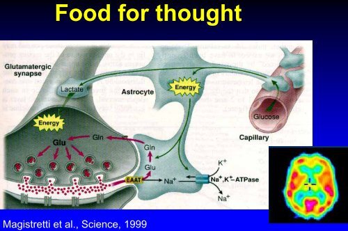
Food for thought 

Magistretti et al., Science, 1999

Hemodynamic response 

Blood 

flow 

Neuroelectrical 

activity 

Blood flow 

Oxygen 

Hemoglobin 

fMRI signal 

Deoxyhemoglobin

Questions about the integration of 

EEG/MEG with the fMRI 

What are the techniques to usefully relate 

EEG/MEG and fMRI 

What is the evidence for true synergy 

What behavioral and analysis methods are 

successful 

What do we expect in the near future

Human brain produces 

measurable signals on the scalp 

Hans Berger in 1929 produced the first report 

on the measurement of electrical activity in 

man over the scalp surface 

He hoped that EEG could represent a sort of 

“window on the mind” 

Berger’s equipment

High Resolution 

Electroencephalography (HREEG) 

Brain activity elicited a time varying 

potential distribution over the 

cortical surface 

Such potential distribution are still 

measurable at the scalp level 

Due to low scalp conductivity the 

EEG Signal to noise ratio is very 

low 

HREEG => Sampling the potential 

distribution with an high number of 

electrodes, MRI images for realistic 

head modeling and spatial 

deblurring algorithms

teps to improve the spatial details of 

recorded EEG Data 

1975 1993 

1989 1996 

Realistic 

Insert the 

Model Computation 

scalp geometry of of 

The of thickness skull Realistic Head and in dura 

Volume Surface the mater SL in 

Conductor Laplacian computation 

inverse 

calculation

The neuroimaging puzzle 

Different neuroimaging techniques, same 

experimental paradigm 

(unilateral right middle finger movement) 

fMRI EEG MEG

The linear inverse problem 

ξ = argmin ( Ax − b + 

The difference between 

modeled and measured 

potentials/fields is 

minimized, together 

with the energy of the 

sources 

x 

2 

M 

λ 

2 

A is the lead field matrix 

x is a vector in the source space 

b is the measured data vector 

λ is a regularization parameter 

M is the metric for the data space 

N is the metric for the source 

space 

ξ is the solution vector 

Solutions ξ are obtained by using x = G b where 

G 

( ) AN 

−1 

′ + λ 

−1 

1 

−1 − 

= N A′ 

A M 

x 

2 

N 

)

Dipolar Localization Error (DLE) 

k-th source 

x 

Est 

= 

Gb 

= 

GAx 

True 

i-th source 

x 

Est 

= 

Rx 

True 

x = Rδ = R. 

i-th column of the resolution matrix R 

iˆ = 

Est 

DLE 

arg 

i 

i 

i 

index of the maximum of the 

max R 

ki 

k 

r = − 

r 

i 

r 

iˆ 

i-th column of the resolution matrix R 

distance between the two sources

Resolution Kernels 

k 

i 

j 

x 

Est 

i 

= 

N 

∑ 

k 

= 1 

R 

ik 

x 

True 

k 

The R ik s define how the different sources other than the i-th 

contributed to the estimation to the i-th itself 

The R ik s belongs to the i-th row of the resolution matrix and 

are called Resolution Kernels

The Resolution Kernel 

Bad Resolution 

Kernel 

large peak around 

the maximum 

one or more peaks 

located far from the 

source position 

Good Resolution Kernel 

narrow peak around 

the maximum 

one peak located at 

the source position

From current strength to probability maps 

How obtain a measure of the uncertainty of current 

estimations due to the EEG/MEG noise (n) 

Under the null hypothesis of 

no activation the Z is 

distributed as a Gaussian 

distribution 

In the case of three 

component for each dipole 

the q as a sum of squares is 

distributed as a Fisher 

distribution (F 3,n ) 

σ 

Z 

q 

i 

i 

2 

Noise 

( t) 

= 

( t) 

= 

= 

⎡ 

⎢ 

⎣ 

G 

Gnn 

3 

k = 1 

3 

k = 1 

GCG 

∑ 

∑ 

G 

G 

k 

' G 

⋅ b( 

t) 

k 

⋅ 

' 

⋅ 

' 

⎤ 

b( 

t) 

⎥ 

⎦ 

C 

= 

⋅ 

GCG 

G 

k 

2 

' 

'

Dale et al., 2000 

From current strengths to 

probability maps 

Point spread functions (DLE) 

Distribution of the PSF (DLE)



Actual dipole position 

Weighted minimum norm 

Resolution kernel 

Noise normalized 

Resolution kernel

From scalp to cortical EEG in RoIs 

Scalp EEG 

Linear inverse estimates 

within a RoI are collapsed 

(mean) 

M1 Hand 

area RoI 

“Virtual” electrode

Integration of EEG and MEG data 

EEG 

MEG


Why: 

Different sensitivities to the neural sources 

Increased amount of information 

Question:How we can fuse femtoTesla and 

microVolt 

Answer: normalizing the measures with noise 

standard deviation 

How: 

Mahalanobis metric for data space 

Column normalization for the source 

space 

ξ = argmin( Ax−b 

+ 

x 

2 

M 

λ 

2 

x 

2 

N 

)


20 ms 23 ms 18..24 ms 

EEG 

SEPs 

MEG 

SEFs 

EEG + 

MEG 

Fuchs et al., 

EEG J., 1998

The EEG and MEG movement-related 

recordings

EEG, MEG and 

EEG/MEG indexes 

Liu et al., 2000 

Babiloni et al., 2000

Left S1 Left M1 Right S1 

Right M1 SMA 

EEG/MEG integration 

EEG MEG EEG/MEG 

EEG MEG EEG-MEG

Integration of EEG or MEG data 

with fMRI 

EEG 

fMRI 

MEG

Combining EEG and/or MEG with fMRI 

Why: 

Different spatial resolution 

Different time resolution 

• How: 

• Mahalanobis metric for the data space (M) 

• Metric on the source space (N) that takes into 

account: 

• visibility from the sensors (column normalization); (|| A .i || 2 ) 

• source activity as expressed by fMRI signal α; g(α)

Dale et al., Neuron, Vol. 26, 55–67, April, 2000, 

Integration of MEG and fMRI 

fMRI solutions 

MEG solutions 

fMRI-constrained MEG solutions

Combining EEG or MEG with fMRI 

Solutions ξ are obtained by using x = G b where 

G 

Proposed metric for integration of EEG, MEG and fMRI data 

A. 

i 

N = 

2 

= 

ii 

1+ 

Kα 

Solution of the electromagnetic inverse problem with fMRI 

constraints when Kα >> 1 

Solution of electromagnetic inverse problem without fMRI 

constraints when Kα

Block-design fMRI signals 

Information on hemodynamic behaviour of 

cortical sources are provided on a temporal 

scale of minutes 

Diagonal metric N 

N 

4% 

0% 

Percent changes (α) 

− 1 

= 

ii 

A 

( α ) 2 

− 

. 2 

g 

i 2 i

Event-related fMRI signals 

1.03 

1.025 

1.02 

strength 

1.015 

1.01 

1.005 

1 

0.995 

0.99 

0.985 

EMG onset 

1 2 3 4 5 6 7 8 

seconds 

S1 

M1 

i j 

Hemodynamical behavior estimated by the correlation between the eventrelated 

fMRI signals from the cortical areas i and j on a seconds scale 

Full source metric N 

N 

ij 

−1 

= 

A. 

i 

2 

−1 

⋅ 

A. 

j 

2 

−1 

⋅ 

g 

( ) ( ) α ⋅ g α ⋅Corr 

( i, 

j) 

i 

j

Temporal domain: 

movement onset (0 msec) 

fMRI 

no fMRI diag fMRI corr fMRI 

4% 

0% 

Percent changes 

+100% Positive -100% Negative 

Unilateral right middle finger movement

Temporal domain: 

reafference peak (+110 msec) 

fMRI 

no fMRI diag fMRI corr fMRI 

4% 

0% 

Percent changes 

+100% Positive -100% Negative 

Unilateral right middle finger movement

Movement-related cortical dynamics 

HREEG 

HREEG 

+ fMRI

From current strength to probability maps 

How obtain a measure of the uncertainty of current 

estimations due to the EEG/MEG noise (n) 

Under the null hypothesis of 

no activation the Z is 

distributed as a Gaussian 

distribution 

In the case of three 

component for each dipole 

the q as a sum of squares is 

distributed as a Fisher 

distribution (F 3,n ) 

σ 

Z 

q 

i 

i 

2 

Noise 

( t) 

= 

( t) 

= 

= 

⎡ 

⎢ 

⎣ 

G 

Gnn 

3 

k = 1 

3 

k = 1 

GCG 

∑ 

∑ 

G 

G 

k 

' G 

⋅ b( 

t) 

k 

⋅ 

' 

⋅ 

' 

⎤ 

b( 

t) 

⎥ 

⎦ 

C 

= 

⋅ 

GCG 

G 

k 

2 

' 

'

Dale et al, Neuron,2000 

Liu, 2000, PhD thesis 

Temporal domain: from current strength 

to probabilistic map 

n i 

(t) 

b i 

(t) 

G 

i-th dipole 

σ 

Z 

2 

Noisei 

i 

( t) 

= 

= 

[ Gnn' 

G' 

] = [ GCG' 

] 

[ G ⋅b( 

t) 

] 

i 

[ GCG' 

] i 

i 

i

Dale et al., 2000 



Point spread functions (DLE) 

Distribution of the PSF (DLE)



Actual dipole position 

Weighted minimum norm 

Resolution kernel 

Noise normalized 

Resolution kernel

Movement-related cortical dynamics 

-0.4 

-5000 -4000 -3000 -2000 -1000 0 1000 2000 3000 

-15 

-5000 -4000 -3000 -2000 -1000 0 1000 2000 3000 

+100% 

Z=10 

t= +50 ms 

Current 

density 

strength 

0.3 

0.2 

0.1 

0 

-100% 

M1 

S1 

SMA 

S1 IPSI 

M1 IPSI 

Z=-10 

Z score 

10 

5 

0 

fMRIconstrained 

fMRIconstrained 

Noisenormalized 

M1 

S1 

SMA 

S1 IPSI 

M1 IPSI 

-0.1 

-0.2 

-0.3 

-5 

-10

Frequency-based linear inverse source 

EMG onset 

estimation 

Alpha desync. 

average 

ERD 

b i 

(t) 

bCSD ( t) 

bCSD 

ij 

ii 

f 

( f ; T ) ≡ B ( f ; T ) ⋅ B ( f ; T 

i 

j 

* 

) 

x( 

t) 

= 

G ⋅b( 

t) 

G 

xCSD ( 

f 

= 

⋅bCSD 

( f 

) 

) ⋅G′

Frequency domain: from current 

strength to probabilistic map 

G 

bCSD (∆t) 

ii 

f 

i-th dipole 

σ 

Z 

2 


i 

( ∆t, 

= Var( 

bCSD 

f ) = 

ii 

( Τ, 

f )) 

[ G⋅bCSD 

( ∆t, 

f ) G' 

] 

σ 

ii 


i

HREEG-Movies

Conclusions 

High resolution EEG improved spatial details of the 

raw EEG potential distributions with respect to the 

standard EEG techniques 

Multimodal integration of high resolution EEG data 

with those provided by MEG and fMRI techniques is 

possible in the framework of linear inverse problem 

Information about sources correlation estimated 

from event-related fMRI can be inserted in the 

solution of the linear inverse problem by using a full 

source metric N

Filippo Carducci 

Claudio Babiloni 

Febo Cincotti 

Fabio Babiloni

Presentation - What is Neuro-iT.net

You also want an ePaper? Increase the reach of your titles

Delete template?

Save as template?