Absolute Stability of a longitudinal Blended Wing Body Aircraft ...

Absolute Stability of a longitudinal
Blended Wing Body Aircraft Model with
Rate Limiting of the Actuator ⋆
Claudia Alice State ∗
∗ Doctoral School of Control Engineering and Computers,
University of Craiova, A.I.Cuza, 13, Craiova, RO-200585, Romania
(e-mail: cldstate@ yahoo.com).
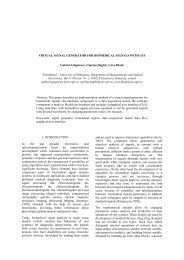
Abstract: This paper is focused on P(ilot) I(n-the-Loop) O(scillations) of Category II
associated to quasi-linear models, which are induced by nonlinearities determined by the
saturation of position or rate limited elements. The theoretical model of the airplane is a Blended
Wing Body (BWB) configuration and the human operator is expressed by the Synchronous Pilot
Model, represented by a simple gain. The absolute stability for the longitudinal BWB aircraft
model proposed is investigated using a frequency Popov-type criterion. The mathematical model
presented in this article is a pilot-aircraft coupled system used for describing the longitudinal
motion of the Blended Wing aircraft and techniques from the frequency domain are applied. The
transfer function obtained from open-loop analysis has a double pole at the origin. Therefore,
the pilot-aircraft system is in the critical case of a double zero root and the Popov criterion, in
the case of the infinite parameter, is applied in order to investigate the absolute stability for the
longitudinal BWB aircraft model in the presence of the rate saturation of the actuator.
Keywords: Absolute stability, Popov criterion, Nonlinear system, Blended Wing Body,
Frequency domain inequality
1. INTRODUCTION
Known to have been the cause for several aircraft incidents
and accidents, the pilot-induced oscillations (PIO)
are dangerous and complicated interactions between the
human pilot and the aircraft dynamics that can lead to
destruction of the aircraft, and it often occurs when the
pilot of an aircraft proves to be unable to adapt himself
to a sudden change of the vehicle dynamics during a high
demanding flight task.
A PIO event can be considered as a closed-loop instability
caused by dynamic coupling between the pilot and the
aircraft, which is described in the specific literature as
”sustained or uncontrollable oscillations resulting from
efforts of the pilot to control the aircraft” (Jeram and
Prasad (2003)) or ”inadvertent, sustained aircraft oscillation
which is the consequence of an abnormal joint enterprise
between the aircraft and the pilot” (McRuer (1992)).
According to common references (see, for example, McRuer
et al. (1996)), PIOs can be separated into four categories.
PIO Category I mainly concerns to linear pilot-vehicle
system oscillations. These PIOs result from linear phenomena
such as excessive lags introduced by filters,
actuators, feel system and digital system time delays.
They are the simplest to model and prevent.
PIO Category II is characterised by quasi-linear pilotvehicle
models, but with some nonlinear contribution,
⋆ This work has been partly supported by the Research Project
CNCSIS ID-95
such as rate or position limiting. The closed loop pilotvehicle
system has a nonlinear behavior, mainly characterized
by the saturation of position or rate limited
elements.
PIO Category III is enough evasive defined as completely
nonlinear. The closed loop pilot-vehicle system has a
highly non-linear behaviour, with no further peculiar
characteristic. These severe life-threatening PIOs are
caused by nonlinearities and transitions in pilot or
effective airplane dynamics.
PIO Category IV which refers to coupling effects between
pilot inputs and the aircraft structural modes, is
characterised by highly non-linear pilot-vehicle system
oscillations. These PIOs are theoretically considered and
less studied.
This paper deal with the analysis of Category II PIOs,
which are mainly characterised by nonlinearities determined
by rate or position saturations of control surface actuators.
Caused by dynamic coupling between the human
pilot and the aircraft, these oscillations can occurs with
motions about all or any symmetry axes of the aircraft,
and this could lead to instability in the systems.
One of the goal of this paper is to provide a frequency criterion
to establish whether a given aircraft is free from PIO
of Category II. Pilot-in-the-loop analysis of the aircraft
dynamics involves adoption of mathematical models of the
human pilot, which can be a useful tool for predicting
these PIOs. The theoretical model of the airplane is a
Blended Wing Body (BWB) tailless configuration which is
claimed to have a superior aerodynamic performance. As
54

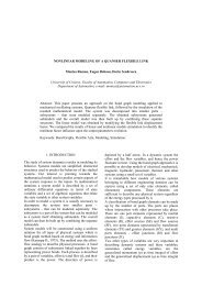
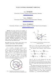
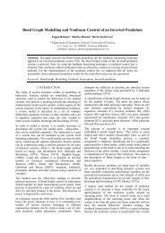
Fig. 2. Simplified actuator model with rate limiting
Fig. 1. BWB concept aircraft
a mathematical model of the human pilot, Synchronous
Pilot Model is considered, represented by a simple gain.
1.1 BWB concept
Defined as having no definite fuselage and only a single
wing, the Blended Wing aircraft generate less noise and
offers a greater lift-to-drag ratio than traditional aircraft.
The BWB aircraft model also offers a reduction in the
number of parts required relating to reduced manufacturing
costs. Figure 1 ilustrates a representative BWB tailless
aircraft.
An intuitive presentation of the BWB concept can be
found in (Chambers (2005)). Also, several researches regarding
this particular configuration are, for example,
(Rahman and Whidborne (2008)) and (Smith and Abbasi
(2004)).
The aerodynamic BWB model used here was obtained taking
into consideration (Castro (2003)) and (Rahman et al.
(2009)). The linear low order BWB aircraft model for the
uncoupled longitudinal dynamics was considered taking
into account the case of short-period approximation. In
addition, only elevator control δ e was retained.
1.2 Actuator Rate Limiting
For absolute stability analysis, the nonlinear equations
of motion describing the aircraft dynamics were obtained
using the rate limiting of the actuator, representing the
nonlinear part of the longitudinal model presented in this
article.
Rate limiting of the actuator is one of main factors
contributing to Category II PIO. A block diagram of a
basic rate-limited actuator model is presented in Figure 2,
where the pilot input command u to the actuator produces
the actual actuator deflection. The output deflection δ is
fed back to the input surface command to produce an
error signal. In the forward path the error signal serves as
the input to the nonlinear saturation block. Actuator rate
limiting occurs when pilot input command error requires
a higher rate than the actuator can actually provide. The
output from the saturation block is the surface rate ˙δ. This
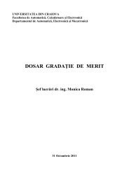
Fig. 3. Saturation nonlinearities
signal is then integrated to produce the surface deflection
δ.
Rate limiting introduces additional phase lag, increasing
the delay between the pilot input command and aircraft
response. Depending upon the characteristics of the aircraft,
this alone can be sufficient to lead to PIO events
and tends to destabilize the closed-loop system.
2. THEORETICAL BACKGROUND
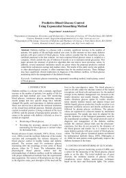
General stabilization of the pilot-aircraft system, using the
rate limiter is shown in the Figure 5, in which the limiter
is of ”AIAA type”, as in (Răsvan (2011)).
In Figure 5, r = 0 represents the null reference and the
following elements are used:
• χ is the output of the system;
• k p represents the model of pilot;
• δ p is the control signal elaborated by the pilot;
• G(s) is the open-loop transfer function for the aircraft
model, where
G(s) =c T (sI − A) −1 b
• ψ designate a non-linear function (a saturation, like in
Figure 3), which fulfills the following sector condition
0 ≤ ¯ψ ≤ ψ(y)
y
≤ ¯ψ ≤∞, ψ(0)=0
where ψ, ψ and y can be seen in Figure 4.
55

Fig. 5. The block diagram of the generic coupled pilotaircraft
system with rate limiter
• x α (t) =[x β (t) δ e (t)] and c T α(t) =[c T β ω 0 ω 0 ].
Fig. 4. Sector restricted nonlinearity
2.1 Nonlinear feedback analysis - The Lurie problem
Absolute stability problem (see (Răsvan (1975)) and
(Răsvan and Danciu (2011))) refers to the global asymptotic
of the zero equilibrium of the general nonlinear system
ẋ(t) =Ax(t) − bψ(c T x(t)) (1)
having sector of restricted nonlinearities of the form
0 ≤ ψ ≤ ψ(y) ≤ ψ ≤ +∞,ψ(0) = 0 (2)
y
and the property of the equilibrium being valid for all the
linear and nonlinear functions verifying (1).
Further details about the global asymptotic stability property
of dynamical systems can be also found in (Voicu
(1986)).
From Figure 5 we can observe that in the feedback structure
composed of the aircraft and human pilot dynamic,
a saturation nonlinearity occurs. An early nonlinear feedback
system analysis problem was formulated by Lurie.
The following transformation of the system who has rate
saturation can be written as in Figure 6. In the example
considered in this paper we can use the following equivalence
between the systems (3) and (4).
ẋ α (t) =A α x α (t) − b α ψ(y(t)) (3)
where
and
where
y(t) =c T αx α (t)
{
ẋβ (t) =A β x β (t)+b β δ e (t)
˙δ e (t) =−ψ(ω 0 (c T β x β (t)+δ e (t)))
(4)
• δ e was introduced as a state;
• A β should be Hurwitz matrix to make sure of the
stability of the system;
• c β ,A β ,b β are smaller in dimension than in (3);
Noting that {
y(t) =ω0 (c T β x β (t)+δ e (t))
u(t) =−ψ(y(t))
and substituting (5) into the system (4), the simplified
system below is obtained:
{
ẋβ (t) =A β x β (t)+b β δ e (t)
(6)
˙δ e (t) =u(t)
Applying the Laplace transformation we obtain:
{
s˜xβ (s) =A β ˜x β (s)+b β ˜δe (s)
s˜δ e (s) =ũ(s)
and
(5)
(7)
ỹ(s) =ω 0 (c T β ˜x β (s)+˜δ e (s)) (8)
From (7) results:
{ ˜xβ (s) =(sI − A β ) −1 b β ˜δe (s)
˜δ e (s) = 1 s ũ(s) (9)
From the above system is obtained:
˜x β (s) = 1 s (sI − A β) −1 b β ũ(s) (10)
From (8), (9) and (10) results
ỹ(s) =c T β (sI − A β ) −1 ω 0
b β
s ũ(s)+ω 0 ũ(s) (11)
s
Using the notation
G(s) =c T β (sI − A β ) −1 b β (12)
from (11) and (12) the following relation is determined
G(s)+1
ỹ(s) =ω 0 ũ(s) (13)
s
which is equivalent to
ỹ(s) =T(s)ũ(s) (14)
The transfer function T (s) (in the case of rate limiter) is
T (s) = ỹ(s) ( 1
ũ(s) = ω 0
s + G(s) )
(15)
s
This shows clearly that the system is in the critical case
of a single zero root - H(s) has a pole at s=0.
56

For the above formally obtained relation, applying the
limit ξ →∞, yields to:
−ωIm [T (jω)] > 0, ∀ω ≥ 0 (20)
3. THE ABSOLUTE STABILITY OF THE
LONGITUDINAL BWB MODEL
Fig. 6. Absolute stability feedback structure
We can observe that the control system from Figure 5 is
transformed into the terms of Lurie feedback connection,
as in Figure 6, where the feedback structure of the absolute
stability contains the saturation nonlinearity ψ. In the
case under study, the block L from the forward path
represents the linear differential equations of the model
and the nonlinear block N represents the rate saturation
of the actuator.
2.2 The Popov criterion
The Popov criterion used in this paper in order to provide
the absolute stability of the longitudinal BWB model with
rate limited actuator, considers the stability of the Lurie
system. For practical considerations the following expression
of Popov criterion is used (from (Sastry (1999))).
Theorem 1. Consider a Lurie system with a nonlinearity
ψ in the sector. The equilibrium in the origin is globally
asymptotically (exponentially) stable, provided that there
exists ξ>0 such that the following inequality is true:
1
+ Re [(1 + jωξ)T(jω)] > 0, ∀ω ∈ R (16)
k
The Popov condition express a frequency condition for the
global asymptotically stability property of a dynamically
system in the condition of the Lurie problem (Khalil
(2002)).
Remark 2. From the general theory of functions of a complex
variable with real coefficients (for example rational
meromorphic functions) it is known that the real part
of a transfer function is even (in ω) and the imaginary
part is odd (but when multiplied with jω it is also even),
so results that the above relation is even and then the
condition ω ≥ 0 is not restrictive:
1
+ Re [(1 + jωξ)T(jω)] > 0, ∀ω ≥ 0 (17)
k
Remark 3. k is the lenght of the sector defined by:
k = ¯ψ − ψ = V L − 0=V L (18)
where V L is the rate limit value.
One should note that in relation (17), by multiplying with
1
ξ
(if ξ > 0) which is a positive quantity, the following
inequality is equivalent.
1
kξ + 1 Re [(1 + jωξ)T(jω)] =
ξ
1
kξ + 1 (19)
ξ Re (T (jω)) − ωIm (T (jω)) > 0
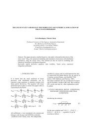
In this section symbolic and numeric computations for the
longitudinal BWB system were performed. The longitudinal
motion of the BWB aircraft model is a dynamical
simplified system with one input (the elevator deflection
δ e ) and two state variables (the angle of attack α and the
pitch rate q). The longitudinal aerodynamic parameters of
the aircraft equations of motion which are time-invariant
are substituted by their numerical values.
3.1 The linear system
Taking into account (Castro (2003)) and (Rahman et al.
(2009)), we consider the following differential equations
of longitudinal motion describing the mathematical BWB
short-period aircraft model:
{
˙α = q
˙q = M q q − M δe δ e
(21)
The linear model for the mentioned uncoupled longitudinal
dynamic can be expressed as
ẋ = Ax + Bu (22)
where
• A and B[ matrices ] are given [ by ]
0
0 1
B = and A =
M δe 0 M q
Introducing the elevator equation into the above system,
the following short-period model with actuator unsaturated
is
⎧
obtained:
⎨ ˙α = q
˙q = M q q − M δe δ e
(23)
⎩ ˙δ e =(−ω 0 )[(k α + k p )α + k q q + δ e ]
where we have:
• α is the incidence angle [rad]
• q represents the pitch rate [rad/s]
• δ e is the elevator deflection [rad]
3.2 The Routh-Hurwitz criterion
At this point, by using the Routh-Hurwitz criterion, can
be verified the stability of the linear system (23). The
characteristic equation is
P (s) =s 3 + a 2 s 2 + a 1 s + a 0 = 0 (24)
where the following notations were made:
{
a2 = ω 0 − M q
a 1 = ω 0 (k q M δe − M q )
(25)
a 0 = ω 0 (k α + k p )M δe
Remark 4. The value of the pilot gain k p is set to unity
and the following global gains of the system and their
57

numerical values are also used:
• k α = −0.526
• k q = −1.27
The aerodynamic constants of the system can be numerically
substituted and are expressed by(from (Rahman
et al. (2009))):
• ω 0 =20 rad
sec
• M q = −0.1556
• M δe = −1.3495
Further, the Hurwitz criterion gives the following conditions:
ω 0 − M q > 0 (26)
ω 0 (k α + k p )M δe > 0 (27)
(ω 0 − M q )(k q M δe − M q ) − (k α + k p )M δe > 0 (28)
It is easy to verify that these conditions are fulfilled.
3.3 Nonlinear model of the BWB aircraft
In Figure 5 from section 2, the general representation of
the pilot-aircraft system is shown.
By adding the rate limited actuator and the SAS (stability
augmentation system) to the linear aircraft equations, the
following pilot-aircraft nonlinear system is obtained:
⎧
⎨
⎩
˙α = q
˙q = M q q − M δe δ e
˙δ e = −ψ(σ)
(29)
where we have the output of the linear system
σ = ω 0 [(k α + k p )α + k q q + δ e ] (30)
and the nonlinearity
{
σ, if | σ |≤ eL
ψ(σ) =
(31)
e L sgnσ, if | σ |> e L
Remark 5. σ is the additive input value and e L is the limit
for saturation ψ. This saturation is crucial for oscillations,
often complicating the effect of PIOs.
Using the notation u = −ψ(σ), like in subsection 2.1, it is
equivalent to rewrite the system (29) as follows
⎧
⎨
⎩
˙α = q
˙q = M q q − M δe δ e
˙δ e = u
(32)
The system below is obtained by applying the Laplace
transform to differential equations system (32)
⎧
˜α(s) = 1 ⎪⎨ s ˜q(s)
˜q(s) =
M δ e ˜δe (s)
(33)
s − M q
⎪⎩ ˜δ e (s) = 1 s ũ(s)
˜δ e is substituted into the second equation of the system
(33), and then ˜q is also substituted into the first equation
of the same system.
So, results
⎧
M δe
˜α(s) =
⎪⎨ s 2 (s − M q
M )ũ(s)
δe
˜q(s) =
s(s − M q )ũ(s)
(34)
⎪⎩ ˜δ e (s) = 1 s ũ(s)
and from (30) was obtained
˜σ(s) =ω 0
[ (kα + k p )M δe
s 2 (s − M q )
where
T (s) = ˜σ(s)
ũ(s)
+ k qM δe
s(s − M q ) + 1 ]
ũ(s) (35)
s
(36)
is the transfer function of the linear part of the system
(29).
3.4 Stability analysis using the Popov criterion
From (35) and (36) the loop transfer function of the
longitudinal BWB nonlinear system (with rate limiter) is
given by
T (s) =ω 0
s 2 +(k q M δe − M q )s +(k α + k p )M δe
s 2 (s − M q )
(37)
From (37) it is clear that the characteristic equation has
a double zero root and the criterion mentioned is used in
this critical case of the absolute stability.
Making the substitution s = jω, we obtain the frequencydomain
transfer function
T (jω)=ω 0
−ω 2 +(k q M δe − M q )jω +(k α + k p )M δe
ω 2 (M q ) − jω
(38)
The transfer functin can be written as follows:
T (jω)=P (ω)+jQ(ω) (39)
where P (ω) şi Q(ω) are defined by
P (ω) =Re(T (jω) (40)
and
Q(ω) =Im(T (jω) (41)
For the Popov condition (20) from subsection 2.2, we have
Q(ω) =ω 0
−ω 2 + k q M δe M q − M 2 q +(k α + k p )M δe
ω(ω 2 + M q 2 )
(42)
In order to apply the Popov frequency-domain inequality,
a straightforward computation will give
−ωIm[T (jω)] = ω 0
ω 2 + P k + M q
2
ω 2 + M q
2
(43)
where, to simplify the writing, P k is denoted by
P k = −(k α + k p + k q M q )M δe (44)
In the presented case, the frequency-domain condition can
be written as:
]
P k
ω 0
[1+
ω 2 2
> 0, ∀ω ≥ 0 (45)
+ M q
which holds if P k > 0.
58

But taking into account that
P k =0.9063 > 0 (46)
it follows that the frequency domain inequality (45) is true.
The limits from below are computed:
lim −ωIm[T (jω)] = ω 0 > 0 (47)
ω→∞
and
lim −ωIm[T (jω)] = ω [
2
0 1+Pk M ] q (48)
ω→0
Numerically, taking into consideration that P k > 0, it is
easy to verify that
lim −ωIm[T (jω)] > 0 (49)
ω→0
Therefore, from (45), (47) and (48) it results that the
Popov frequency-domain inequality is satisfied, in the
case of the infinite Popov parameter. It follows that the
absolute stability of the longitudinal BWB model with rate
limiter actuator was proved, in the specified conditions,
using the Popov criterion.
Răsvan, V. (2011). Systems with monotone and slope
restricted nonlinearities. Tatra Mountains Mathematical
Publications. Volume 48, No.1, 165–187.
Răsvan, V. and Danciu, D. (2011). Theoretical background
for pio ii analysis. Scientific Bulletin of Politehnica
University of Timisoara, Romania, Transactions on Automatic
Control and Computer Science. Vol. 56(70),
No. 1, March 2011, pp. 5-10, Politehnica Publ. House,
ISSN 1224-600X.
Sastry, S. (1999). Nonlinear systems; analysis, stability
and control. ISBN 0-387-98513-1.
Smith, H. and Abbasi, Y. (2004). The mob blended
wing body reference aircraft. Technical report. Cranfield
University, 71–92.
Voicu, M. (1986). Stability Analysis Techniques of the
Automatic Control Systems (in Romanian). Editura
Tehnică, Bucureşti.
4. CONCLUSION
For the BWB configuration, the low order pilot-aircraft
system is absolutely stable with the influence of actuator
nonlinearity, in the mentioned conditions. As a future work
it can be considered the analysis of the models that are
more complex in representation, in the presence of more
non-linearities of the systems.
REFERENCES
Castro, H.V. (2003). Flying and Handling Qualities of a
Fly-By-Wire Blended Wing Body Civil Transport Aircraft,
PhD. Thesis. Cranfield University, England.
Chambers, J.R. (2005). Innovation in flight. NASA SP-
2005-4539, Boston.
Jeram, G.J. and Prasad, J.V.R. (2003). Tactile avoidance
cueing for pilot induced oscillation. Proc. AIAA Atmospheric
Flight Mechanics Conference and Exhibitt, 1–9.
Khalil, H.K. (2002). Nonlinear systems. 3rd edition. ISBN
0-13-067389-7.
McRuer, D. (1992). Human dynamics and pilot-induced
oscillations. Massachusetts Institute of Technology,
Cambridge, MA.
McRuer, D., Klyde, D.H., and Myers, T.T. (1996). Development
of a comprehensive pio theory. Proc. AIAA
Atmospheric Flight Mechanics Conference, 581–597.
Rahman, N.U. and Whidborne, J.F. (2008). A lateral
directional flight control system for the mob blended
wing body platform. UKACC Int. Conf. CONTROL.
Rahman, N.U., Whidborne, J.F., and Cooke, A.K. (2009).
Longitudinal control system design and handling qualities
assessment of a blended wing body aircraft. The
6th International Bhurban Conference on Applied Sciences
and Technology (IBCAST). Dept. of Aerosp. Sci.
Cranfield Univ.
Răsvan, V. (1975). Absolute stability of time lag control
systems. 1st ed. Bucharest: Editura Academiei, (in
Romanian).
59