Planar Linkage Analysis using GeoGebra
Planar Linkage Analysis using GeoGebra
Planar Linkage Analysis using GeoGebra

Create successful ePaper yourself
Turn your PDF publications into a flip-book with our unique Google optimized e-Paper software.
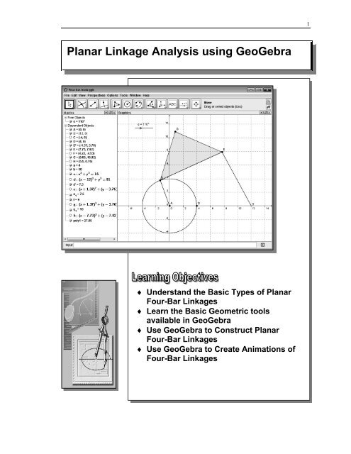
<strong>Planar</strong> <strong>Linkage</strong> <strong>Analysis</strong> <strong>using</strong> <strong>GeoGebra</strong><br />
� Understand the Basic Types of <strong>Planar</strong><br />
Four-Bar <strong>Linkage</strong>s<br />
� Learn the Basic Geometric tools<br />
available in <strong>GeoGebra</strong><br />
� Use <strong>GeoGebra</strong> to Construct <strong>Planar</strong><br />
Four-Bar <strong>Linkage</strong>s<br />
� Use <strong>GeoGebra</strong> to Create Animations of<br />
Four-Bar <strong>Linkage</strong>s<br />
1
2<br />
Introduction to Four-Bar <strong>Linkage</strong>s<br />
A machine is a system or device consisting of fixed and moving parts that modifies<br />
mechanical energy to do work. Assemblies within a machine that control movement are<br />
often called mechanisms. A mechanism is a group of links connected together for the<br />
purpose of transmitting forces or motions. A four-bar linkage or four-bar mechanism<br />
is the simplest movable mechanism commonly used in machines. A four-bar linkage<br />
consists of four rigid bodies (called bars or links) with one link fixed. The four links are<br />
each attached to two others by single joints (pivots) to form a closed loop. The fixed link<br />
is referred to as the frame; one of the rotating links is called the driver or crank; the<br />
other rotating link is called the follower or rocker; and the floating link is called the<br />
connecting rod or coupler. Some of the more commonly used four-bar linkages are<br />
listed below.<br />
� Depending upon the arrangement and lengths of the links, different types of<br />
motions can be generated. Different mechanisms can also be formed by fixing<br />
different links of the same chain.<br />
Crank-Rocker<br />
� The Crank-Rocker<br />
mechanism is a four-bar<br />
linkage in which the shorter<br />
link makes a complete<br />
revolution and the opposite<br />
link rocks (oscillates) back<br />
and forth.
Crank-Rocker<br />
� The Double-Crank or Drag-<br />
Link mechanism is a four-bar<br />
linkage with two opposite links<br />
making complete revolutions.<br />
Double-Crank<br />
Double-Rocker<br />
<strong>Planar</strong> <strong>Linkage</strong> <strong>Analysis</strong> with <strong>GeoGebra</strong> 3<br />
� Note that by fixing the<br />
opposite link of the same<br />
mechanism, another<br />
Crank-Rocker<br />
mechanism is formed.<br />
� The Double-Rocker<br />
mechanism is a four-bar<br />
linkage in which the crank and<br />
follower rock (oscillate) back<br />
and forth; none of the links can<br />
make full revolution.<br />
� Note the four different<br />
mechanisms above are formed<br />
by fixing different links of the<br />
same links.
4<br />
� The Slider-Crank mechanism is a special case of the four-bar linkage. As the<br />
follower link of a crank-rocker linkage gets longer, the path of the pin joint<br />
between the connecting rod and the follower approaches a straight line. Slider-<br />
Crank is a mechanism for converting the linear motion of a slider into rotational<br />
motion or vice-versa.<br />
Slider-Crank Variation<br />
Scotch Yoke<br />
Slider-Crank<br />
� The Scotch Yoke is<br />
most commonly used<br />
in reciprocating piston<br />
pumps and in control<br />
valve actuators in<br />
high pressure oil and<br />
gas pipelines.
Introduction to <strong>GeoGebra</strong><br />
<strong>Planar</strong> <strong>Linkage</strong> <strong>Analysis</strong> with <strong>GeoGebra</strong> 5<br />
<strong>GeoGebra</strong> is an award winning interactive dynamic geometry software that joins<br />
geometry, algebra and calculus. Interactive dynamic geometry software is a type of<br />
computer program that allows the creation and then manipulation of geometric<br />
constructions. In most interactive geometry software, constructions can be made with<br />
points, vectors, segments, lines, polygons, conic sections, inequalities, implicit<br />
polynomials and functions.<br />
The development of <strong>GeoGebra</strong> was started by Prof. Markus Hohenwarter for<br />
mathematic education. Prof. Markus Hohenwarter started the project in 2001 at the<br />
University of Salzburg, continuing it at Florida Atlantic University (2006–2008), Florida<br />
State University (2008–2009), and now at the University of Linz together with the help of<br />
open-source developers and translators all over the world.<br />
In <strong>GeoGebra</strong>, geometric entities can be entered and modified directly on screen, or<br />
through the Input Bar. <strong>GeoGebra</strong> has the ability to use variables for numbers, vectors and<br />
points; derivatives and integrals of functions can also be evaluated.<br />
The main webpage of <strong>GeoGebra</strong> is at http://www.geogebra.org/cms/en<br />
� <strong>GeoGebra</strong> is an open source free software, written in<br />
Java and thus available for multiple platforms,<br />
including Windows, Mac and Linux systems.
6<br />
� Two versions of <strong>GeoGebra</strong> are available for download. <strong>GeoGebra</strong> is the full<br />
version and <strong>GeoGebra</strong>Prim has the same capabilities as the full version but uses a<br />
more simplified user interface. Files created in <strong>GeoGebra</strong> can be loaded in<br />
<strong>GeoGebra</strong>Prim and vice versa.<br />
� Note the installation of the Java Platform is required as <strong>GeoGebra</strong> is written in<br />
Java.<br />
.<br />
� For most versions of <strong>GeoGebra</strong>, the<br />
installed program can be accessed through<br />
the Start menu or the <strong>GeoGebra</strong> icon on<br />
the desktop.
<strong>Planar</strong> <strong>Linkage</strong> <strong>Analysis</strong> with <strong>GeoGebra</strong> 7<br />
1. Select the <strong>GeoGebra</strong> option on the Start menu or select the<br />
<strong>GeoGebra</strong> icon on the desktop to start <strong>GeoGebra</strong>. The <strong>GeoGebra</strong><br />
main window will appear on the screen.<br />
2. In the View pull-down menu, switch<br />
on the Grid display by clicking on the<br />
icon with the left-mouse-button as<br />
shown.<br />
� The <strong>GeoGebra</strong> screen layout contains the pull-down menus, the Standard toolbar,<br />
the Algebra area, the graphics area, and the Input Bar at the bottom of the screen.<br />
3. On your own, adjust the display of the <strong>GeoGebra</strong> main screen so that the Algebra<br />
area and the Input Bar are available as shown.
8<br />
5. Click on the origin of the<br />
coordinate system to place the<br />
center of the circle. Note the<br />
created center point is also<br />
added in the Algebra area that is<br />
toward the left.<br />
7. Pick OK to accept the selected settings.<br />
9. Use the mouse wheel to<br />
Zoom/Pan and adjust the<br />
current display.<br />
4. Select the Circle with Center and<br />
Radius icon in the Standard toolbar<br />
area.<br />
6. In the Radius input box, enter<br />
4 to create a circle with a<br />
radius of 4 units in size.<br />
8. On your own, create another circle at<br />
coordinates (12,0) and radius 9 units as<br />
shown.
11. Select the X Axis as the first<br />
entity to define the intersection<br />
points.<br />
� Note two intersection<br />
points are created,<br />
Point C and Point D.<br />
<strong>Planar</strong> <strong>Linkage</strong> <strong>Analysis</strong> with <strong>GeoGebra</strong> 9<br />
10. Activate the Intersect Two Objects<br />
command by clicking on the icon as shown.<br />
This will create points at the intersections of<br />
two selected objects.<br />
12. Select the smaller circle<br />
as the second entity to<br />
define the intersection<br />
points.
10<br />
14. Select Point D as the<br />
object to be rotated.<br />
16. In the Angle input box,<br />
enter 45 as the angle of<br />
rotation.<br />
17. Click OK to accept the<br />
setting and create the<br />
new point.<br />
13. Activate the Rotate Object around<br />
Point by Angle command by clicking<br />
on the icon as shown. This will create a<br />
new point by rotating an existing point.<br />
15. Select Point A as the reference<br />
axis of rotation.
19. Select Point DꞋ as the center<br />
of the new circle. Note the<br />
created center point is also<br />
added in the Algebra area<br />
that is toward the left.<br />
21. Click OK to accept the selected settings.<br />
<strong>Planar</strong> <strong>Linkage</strong> <strong>Analysis</strong> with <strong>GeoGebra</strong> 11<br />
18. Select the Circle with Center and<br />
Radius icon in the Standard toolbar<br />
area.<br />
20. In the Radius input box,<br />
enter 10 to create a circle<br />
with a radius of 10 units in<br />
size.<br />
22. Activate the Intersect Two Objects<br />
command by clicking on the icon as shown.<br />
This will create points at the intersections<br />
of two selected objects.
12<br />
24. Select Circle d as the<br />
second entity to define the<br />
intersection points.<br />
23. Select Circle e as the first<br />
entity to define the<br />
intersection points.<br />
� Note two intersection<br />
points are created, Point<br />
E and Point F.
26. Click on Point A to place the<br />
first point of the line.<br />
28. On your own, create two<br />
additional line segments, Line<br />
DE and Line EB as shown.<br />
<strong>Planar</strong> <strong>Linkage</strong> <strong>Analysis</strong> with <strong>GeoGebra</strong> 13<br />
25. Activate the Segment between<br />
Two Points command by<br />
clicking on the icon as shown.<br />
This will create a line by<br />
selecting two endpoints.<br />
27. Click on Point DꞋ to create a line as<br />
shown.
14<br />
Turn off the Display of Objects<br />
2. Select Circle d, the circle<br />
on the right, as shown.<br />
3. Inside the graphics area,<br />
right-mouse-click once to<br />
bring up the option menu.<br />
4. Click the Show Object<br />
icon to turn OFF the display<br />
of the selected circle.<br />
5. Inside the Algebra area,<br />
click once with the rightmouse-button<br />
on Circle<br />
e to display the option<br />
menu. Click on Show<br />
Object to toggle OFF<br />
the display of the circle.<br />
1. In the Standard toolbar area, click on the Move icon to<br />
activate the command.<br />
� Note the corresponding circle,<br />
Circle d, is also highlighted in the<br />
Algebra area. The unfilled icon<br />
indicates the display of the object<br />
has been turned OFF.
8. In the Algebra area, click once with the<br />
right-mouse-button on Point C to<br />
display the option menu. Click on<br />
Show Object to toggle OFF the<br />
display of the selected item.<br />
<strong>Planar</strong> <strong>Linkage</strong> <strong>Analysis</strong> with <strong>GeoGebra</strong> 15<br />
6. Select Point F, the point below the<br />
line segments, as shown.<br />
7. On your own, turn OFF the display of<br />
the object through the right-click option<br />
menu as shown.
16<br />
Adding a Slider Control<br />
2. In the graphics area, select a<br />
location near the upper left corner<br />
to place the Slider Control as<br />
shown.<br />
4. Set the Interval<br />
settings to the three<br />
values, 0, 360 and<br />
1.0, as shown.<br />
5. Click Apply to<br />
accept the selected<br />
settings<br />
1. In the Standard toolbar select the<br />
Slider command by left-clicking<br />
once on the icon.<br />
3. Set the Slider option to Angle as shown.<br />
Note the angle name is automatically set<br />
to α.
<strong>Planar</strong> <strong>Linkage</strong> <strong>Analysis</strong> with <strong>GeoGebra</strong> 17<br />
6. In the Standard toolbar area, click on the Move<br />
icon to activate the command.<br />
7. Drag the handle of the Slider Control, and notice Angle α is<br />
adjusted.<br />
8. In the Algebra area, double click<br />
with the left-mouse-button on<br />
Point DꞋ to enter the Object<br />
Redefine mode.<br />
9. Modify the angle variable, the second variable in the edit box, to α as shown.<br />
10. Click OK to accept the setting and exit the Redefine command.
18<br />
11. Drag the handle of the Slider Control, and notice the positions of the links of<br />
the four-bar linkage are adjusted accordingly.
Using the Animate option<br />
2. Inside the Algebra area, click once with the<br />
right-mouse-button on Angle to display the<br />
option menu. Click on Object Properties<br />
to activate the command.<br />
<strong>Planar</strong> <strong>Linkage</strong> <strong>Analysis</strong> with <strong>GeoGebra</strong> 19<br />
1. Inside the graphics area, click once with the rightmouse-button<br />
on Slider Control to display the<br />
option menu. Click on Animation On to toggle<br />
ON the animation of the Slider Control.<br />
3. Set the animation repeat<br />
option to Increasing as<br />
shown.<br />
4. Click Close to accept the setting and exit the object properties<br />
command.<br />
5. On your own, examine the animation of the four-bar<br />
linkage; turn OFF the animation option before<br />
proceeding to the next section.
20<br />
Tracking the Path of a point on the Coupler<br />
2. Select Point DꞋ as the center of<br />
the new circle.<br />
5. On your own, create<br />
another radius 7.5<br />
circle centered at<br />
Point E as shown.<br />
1. Select the Circle with Center and<br />
Radius icon in the Standard toolbar<br />
area.<br />
3. In the Radius input box,<br />
enter 7.5 as the radius.<br />
4. Click on the OK button to<br />
accept the settings and<br />
create the circle.
7. Select Circle g as<br />
the first entity to<br />
define the<br />
intersection points.<br />
<strong>Planar</strong> <strong>Linkage</strong> <strong>Analysis</strong> with <strong>GeoGebra</strong> 21<br />
6. Activate the Intersect Two Objects command<br />
by clicking on the icon as shown. This will create<br />
points at the intersections of two selected objects.<br />
8. Select Circle h as the<br />
second entity to define<br />
the intersection points.
22<br />
10. Select Point DꞋ as<br />
the first corner of the<br />
polygon.<br />
11. Select Point G as<br />
the second corner of<br />
the polygon.<br />
9. Activate the Polygon command by clicking on the<br />
icon as shown. This will create a polygon by<br />
defining the corner points of a polygon.<br />
12. Select Point E as<br />
the third corner of<br />
the polygon.<br />
13. Select Point DꞋ<br />
again to form a<br />
triangle.<br />
14. On your own, turn<br />
OFF the display of<br />
Point H, Circle g<br />
and Circle h.
16. In the graphics area, select<br />
Point G as shown.<br />
<strong>Planar</strong> <strong>Linkage</strong> <strong>Analysis</strong> with <strong>GeoGebra</strong> 23<br />
15. In the Standard toolbar area, click on the Move<br />
icon to activate the command.<br />
17. Inside the graphics area,<br />
click once with the rightmouse-button<br />
to display<br />
the option menu. Click on<br />
Trace On to activate the<br />
command.<br />
18. Drag the handle of the Slider Control, and notice Angle α is<br />
adjusted.
24<br />
� The locus of point G, also known as a coupler curve, is generated as Angle α is<br />
adjusted. Note that by varying the lengths of the links in the mechanism, different<br />
coupler curves can be generated. The interactive dynamic geometry software can<br />
be used to aid linkage design and analysis.<br />
� Note that the Animation On command can also<br />
be used to generate the coupler curve.
Exercises:<br />
1. Crank-Slider Mechanism<br />
AB = 2.5, BC = 5<br />
2. Watt Straight Line Mechanism<br />
<strong>Planar</strong> <strong>Linkage</strong> <strong>Analysis</strong> with <strong>GeoGebra</strong> 25<br />
ADꞋꞋ=BE, EDꞋꞋ=1/2 ADꞋꞋ, AB = 2 BE, G is at the midpoint of EDꞋꞋ.<br />
A and B are fixed points.
26<br />
3. Hoekens Straight Line Mechanism<br />
BE = ECꞋ = EH = 2.5 ACꞋ, AB = 2 ACꞋ<br />
A and B are fixed points and Link CꞋ-E-H is a rigid link.