Draft revision of the GLORIA Field Manual - The Global Observation ...
Draft revision of the GLORIA Field Manual - The Global Observation ...
Draft revision of the GLORIA Field Manual - The Global Observation ...

You also want an ePaper? Increase the reach of your titles
YUMPU automatically turns print PDFs into web optimized ePapers that Google loves.
<strong>Draft</strong> <strong>revision</strong> <strong>of</strong><br />
<strong>the</strong> <strong>GLORIA</strong> <strong>Field</strong> <strong>Manual</strong>:<br />
Chapter 8 <strong>The</strong> sampling design<br />
June 17 2011<br />
This draft is a follow-up document <strong>of</strong> <strong>the</strong> <strong>GLORIA</strong> conference in Perth/Scotland in<br />
September 2010. At this meeting, attended by <strong>GLORIA</strong> participants from 34 countries<br />
<strong>of</strong> six continents, monitoring methods for <strong>GLORIA</strong>'s Multi-Summit approach were<br />
broadly discussed.<br />
<strong>The</strong> draft update mainly focuses on <strong>the</strong> obligatory part <strong>of</strong> <strong>the</strong> Multi-Summit approach,<br />
where agreements were met at <strong>the</strong> Perth meeting. Optional methods are only briefly<br />
described and are still incomplete.<br />
Updated text is highlighted in blue.<br />
This document (available at: http://www.gloria.ac.at/a=20) should serve for <strong>GLORIA</strong><br />
fieldwork planned in <strong>the</strong> coming months until <strong>the</strong> fully revised 5th version <strong>of</strong> <strong>the</strong><br />
<strong>GLORIA</strong> <strong>Field</strong> <strong>Manual</strong> is published.<br />
Please see also <strong>the</strong> revised sampling forms that can be downloaded at:<br />
http://www.gloria.ac.at/a=51<br />
under: "Download <strong>the</strong> <strong>GLORIA</strong> relevant forms (new version, May 2011)"<br />
<strong>The</strong> full new version (publication is planned for early 2012) also will include optional<br />
methods and additional activities that require fur<strong>the</strong>r discussion and input.<br />
<strong>GLORIA</strong> Coordination<br />
Institute <strong>of</strong> Mountain Research, Austrian Academy <strong>of</strong> Sciences<br />
&<br />
Department <strong>of</strong> Conservation Biology, Vegetation and Landscape Ecology,<br />
University <strong>of</strong> Vienna<br />
Rennweg 14, A-1030 Vienna, Austria<br />
www.gloria.ac.at
<strong>GLORIA</strong> <strong>Field</strong> <strong>Manual</strong> <strong>The</strong> Multi-Summit approach (REVISED DRAFT 2011-06)<br />
8 <strong>The</strong> sampling design<br />
This chapter contains <strong>the</strong> detailed description on how to establish a monitoring site on a mountain<br />
summit. An overview is given below:<br />
8.1 Plot types and design outline 3<br />
8.2 Materials and preparations 4<br />
8.3 <strong>The</strong> set-up <strong>of</strong> <strong>the</strong> permanent plots 5<br />
8.3.1 <strong>The</strong> highest summit point (HSP): determination <strong>of</strong> <strong>the</strong> principal reference point 5<br />
WORKINGSTEP a Marking <strong>the</strong> HSP 5<br />
8.3.2 Establishing <strong>the</strong> 3m x 3m quadrat clusters and <strong>the</strong> summit area corner points 6<br />
WORKINGSTEP b Determination <strong>of</strong> <strong>the</strong> principal measurement line(s) 6<br />
WORKINGSTEP c Fixing <strong>the</strong> 3m x 3m grids <strong>of</strong> <strong>the</strong> quadrat clusters 9<br />
WORKINGSTEP d Measuring distances & magnetic compass direction<br />
from HSP to quadrat clusters 9<br />
8.3.3 Establishing <strong>the</strong> boundaries <strong>of</strong> <strong>the</strong> summit areas and <strong>the</strong> summit area sections 10<br />
WORKINGSTEP e Establishing <strong>the</strong> boundary line <strong>of</strong> <strong>the</strong> 5-m summit area 10<br />
WORKINGSTEP f Establishing <strong>the</strong> boundary line <strong>of</strong> <strong>the</strong> 10-m summit area 11<br />
WORKINGSTEP g Dividing <strong>the</strong> summit areas into sections 11<br />
8.4 Required recording procedures 12<br />
8.4.1 Recording in <strong>the</strong> 1m x 1m quadrats [<strong>the</strong> four corner quadrats <strong>of</strong> <strong>the</strong> four 3m x 3m quadrat clusters in<br />
each main direction (N, E, S, & W), which yields a total <strong>of</strong> 16 quadrats per summit = <strong>the</strong> 16-quadrat area]: 12<br />
8.4.1.1 Visual cover estimation in 1m x 1m quadrats [aim: to detect changes <strong>of</strong> species<br />
composition and cover and changes <strong>of</strong> vegetation cover] 12<br />
WORKINGSTEP h Recording <strong>of</strong> <strong>the</strong> habitat characteristics 12<br />
WORKINGSTEP i Recording <strong>of</strong> <strong>the</strong> species composition and cover 13<br />
8.4.1.2 Pointing with a grid frame in 1m x 1m quadrats [aim: to detect changes in surface types and<br />
species cover <strong>of</strong> <strong>the</strong> more common species, i.e. a second measure <strong>of</strong> vegetation and species cover] 16<br />
WORKINGSTEP j Pointing <strong>of</strong> surface types and vascular plant species 16<br />
8.4.2 Recording in <strong>the</strong> summit area sections [upper (5-m) and lower (10-m) summit area, each divided<br />
into 4 sections = 8 summit area sections; aim: to assess plant migration, to characterise <strong>the</strong> summit habitat] 17<br />
WORKINGSTEP k Complete species list with an estimated abundance <strong>of</strong> each species along an<br />
ordinal scale 17<br />
WORKINGSTEP l Percentage top cover estimation <strong>of</strong> <strong>the</strong> surface types 17<br />
8.4.3 Continuous temperature measurements [Positioning <strong>of</strong> miniature temperature data loggers;<br />
aim: to compare <strong>the</strong> T regimes and to detect <strong>the</strong> snow-cover period along <strong>the</strong> elevation gradient]. 19<br />
WORKINGSTEP m Logger settings and preparations 21<br />
WORKINGSTEP n Positioning <strong>of</strong> <strong>the</strong> data loggers 21<br />
8.4.4 <strong>The</strong> photo documentation [aim: <strong>the</strong> accurate plot reassignment and to document <strong>the</strong> visual situation] 22<br />
WORKINGSTEP o photo documentation <strong>of</strong> <strong>the</strong> HSP 22<br />
WORKINGSTEP p <strong>of</strong> <strong>the</strong> 1m x 1m quadrats 22<br />
WORKINGSTEP q <strong>of</strong> 3 x 3m quadrat cluster (overview) 23<br />
WORKINGSTEP r <strong>of</strong> <strong>the</strong> corner points (summit area sections) 23<br />
WORKINGSTEP s <strong>of</strong> <strong>the</strong> temperature loggers 24<br />
WORKINGSTEP t <strong>of</strong> <strong>the</strong> entire summit 24<br />
OPTIONAL WORKINGSTEP u o<strong>the</strong>r detail photos 24<br />
8.4.5 Removal <strong>of</strong> plot delimitations and considerations for future reassignment 24<br />
WORKINGSTEP v Removal <strong>of</strong> plot delimitations 24<br />
8.4.6 General information on <strong>the</strong> target region 25<br />
WORKINGSTEP w Provide information about <strong>the</strong> target region 25<br />
8.5 Optional recording procedures (incomplete) 27<br />
2
<strong>GLORIA</strong> <strong>Field</strong> <strong>Manual</strong> <strong>The</strong> Multi-Summit approach (REVISED DRAFT 2011-06)<br />
8.1 Plot types and design outline<br />
<strong>The</strong> sampling design for each summit consists <strong>of</strong>:<br />
(a) sixteen 1m x 1m permanent quadrats, arranged as <strong>the</strong> four corner quadrats <strong>of</strong> <strong>the</strong> four 3m x 3m<br />
quadrat clusters in all four main compass directions, yielding 16 1m-quadrats per summit (=16-<br />
quadrat area)<br />
(b) Summit area sections, with 4 sections in <strong>the</strong> upper summit area (5-m summit area) and 4 sections in<br />
<strong>the</strong> lower summit area (10-m summit area). <strong>The</strong> size <strong>of</strong> <strong>the</strong> summit area section is not fixed but<br />
depends on <strong>the</strong> slope structure and steepness.<br />
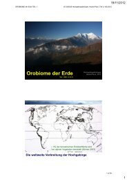
Fig. 8.1 <strong>The</strong> Multi-<br />
Summit sampling design<br />
shown on an example<br />
summit:<br />
(a) oblique view with<br />
schematic contour lines;<br />
(b) top view. <strong>The</strong><br />
3m x 3m quadrat<br />
clusters and <strong>the</strong> corner<br />
points <strong>of</strong> <strong>the</strong> summit<br />
areas are arranged in <strong>the</strong><br />
main geographical<br />
directions. Deviations<br />
from <strong>the</strong> exact direction<br />
(e.g. <strong>the</strong> W-direction in<br />
this example and in Fig.<br />
8.6) may be necessary in<br />
some cases (see<br />
subchapter 8.3.2). Each<br />
quadrat clusters can be<br />
arranged ei<strong>the</strong>r on <strong>the</strong><br />
left or on <strong>the</strong> right side<br />
<strong>of</strong> <strong>the</strong> principal<br />
measurement line,<br />
depending on <strong>the</strong> local<br />
terrain and habitat<br />
situation (this is<br />
independent <strong>of</strong> <strong>the</strong><br />
respective settings <strong>of</strong> <strong>the</strong><br />
o<strong>the</strong>r 3 quadrat clusters).<br />
As a general rule, left<br />
and right is always<br />
defined in <strong>the</strong> sight to<br />
<strong>the</strong> summit.<br />
a)<br />
7m<br />
8m<br />
9m<br />
10m<br />
b)<br />
S<br />
10 m<br />
6m<br />
4m<br />
5m<br />
3m<br />
2m<br />
Highest summit point<br />
1m<br />
Highest summit point<br />
1m<br />
2m<br />
3m<br />
4m<br />
5m<br />
6m<br />
7m<br />
8m<br />
9m<br />
SE<br />
10m<br />
E<br />
Contour line<br />
(referring to<br />
<strong>the</strong> highest summit<br />
point)<br />
Principal<br />
measurement line<br />
Measurement line<br />
for quadrat cluster<br />
corners<br />
3m x 3m<br />
quadrat cluster<br />
with four<br />
permanent quadrats<br />
Boundary <strong>of</strong><br />
summit areas<br />
Upper summit area<br />
= 5-m summit area<br />
Lower summit area<br />
= 10-m summit area<br />
Intersection line<br />
dividing <strong>the</strong><br />
summit area into<br />
sections<br />
An illustration <strong>of</strong> <strong>the</strong> plot arrangements is shown in Fig. 8.1 with an oblique and a top view on an<br />
example summit. Fig. 8.2 shows <strong>the</strong> scheme <strong>of</strong> <strong>the</strong> sampling design with <strong>the</strong> code numbers <strong>of</strong> all<br />
measurement points and sampling plots.<br />
This design was first applied in <strong>the</strong> Nor<strong>the</strong>astern Limestone Alps, Austria (in 1998) and in <strong>the</strong> Sierra<br />
Nevada, Spain (in 1999, PAULI et al. 2003). In 2001, 72 summits throughout Europe were established in<br />
18 target regions along this design as long-term observation sites. Ten years later (2011), <strong>the</strong> number <strong>of</strong><br />
active <strong>GLORIA</strong> target regions has increased to > 90 regions distributed over five continents.<br />
<strong>The</strong> full setup and recording procedure requires between 2 days and about 5 days per summit for a team<br />
<strong>of</strong> four investigators (dependent on vegetation density, species richness and site accessibility). This<br />
estimation includes <strong>the</strong> sampling <strong>of</strong> vascular plants, but excludes <strong>the</strong> recording <strong>of</strong> bryophytes and lichens<br />
on <strong>the</strong> species level.<br />
Note that at least two field workers are absolutely necessary for establishing <strong>the</strong> permanent recording<br />
areas and settings, but a team <strong>of</strong> at least four persons is highly recommended.<br />
3
<strong>GLORIA</strong> <strong>Field</strong> <strong>Manual</strong> <strong>The</strong> Multi-Summit approach (REVISED DRAFT 2011-06)<br />
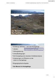
Position <strong>of</strong> <strong>the</strong> corner points<br />
HSP (Highest summit point)<br />
p10m-N<br />
10 m<br />
10-m contour line<br />
Principal<br />
measurement lines<br />
N-10m-SA<br />
p5m-N11<br />
p5m-N31<br />
Measurement lines<br />
from <strong>the</strong> HSP to<br />
3 corner points <strong>of</strong> each<br />
quadrat clusters<br />
pNW-10<br />
p-N33<br />
N31<br />
N33<br />
N11<br />
N13<br />
p-N13<br />
pNE-10<br />
p10m-W<br />
W-10m-SA<br />
p-W13<br />
p5m-W11<br />
p5m-W31<br />
W11 W13<br />
W31 W33<br />
pNW-5<br />
p-W33<br />
W-5m-SA<br />
N-5m-SA<br />
HSP<br />
S-5m-SA<br />
5-m contour line<br />
E-5m-SA<br />
pNE-5<br />
p-E33<br />
p-E13<br />
E33 E31<br />
E13 E11<br />
p5m-E31<br />
p5m-E11<br />
E-10m-SA<br />
p10m-E<br />
N31<br />
N33<br />
N11<br />
N13<br />
pSW-10<br />
3m x 3m quadrat cluster:<br />
four quadrat clusters, each with<br />
four 1m x 1m quadrats =<br />
16 1m² sampling units<br />
(forming toge<strong>the</strong>r <strong>the</strong> 16-quadrat area)<br />
pSW-5<br />
p-S33<br />
p-S13<br />
pSE-5<br />
S13 S33<br />
S11<br />
S31<br />
p5m-S31<br />
p5m-S11<br />
S-10m-SA<br />
p10m-S<br />
pSE-10<br />
Boundary <strong>of</strong><br />
summit areas<br />
(which does not follow<br />
<strong>the</strong> contour line)<br />
Upper summit area<br />
= 5-m summit area<br />
Lower summit area<br />
= 10-m summit area<br />
Intersection lines:<br />
divide <strong>the</strong> summit areas into eight<br />
summit area sections (e.g.<br />
N-5m-SA, N-10m-SA)<br />
<strong>The</strong> corner points:<br />
p10m-N, p10m-E, p10m-S,p10m-W :<br />
<strong>the</strong> 4 corner points at <strong>the</strong> 10-m level; <strong>the</strong>y determine <strong>the</strong> lower<br />
limit <strong>of</strong> <strong>the</strong> 10-m summit area;<br />
<strong>The</strong> principal measurement line for each main direction starts at <strong>the</strong> HSP,<br />
runs through one <strong>of</strong> <strong>the</strong> points at <strong>the</strong> 5-m level (e.g. p5m-N11 or p5m-N31)<br />
and ends at <strong>the</strong> points at <strong>the</strong> 10-m level;<br />
pNE-5, pNE-10, pSE-5, pSE-10<br />
pSW-5, pSW-10, pNW-5,pNW-10 :<br />
<strong>the</strong> 8 corner points at <strong>the</strong> intersection lines<br />
(<strong>the</strong>se points usually lie above <strong>the</strong><br />
5-m level and <strong>the</strong> 10-m level, respectively)<br />
<strong>The</strong> summit area sections are delimited by <strong>the</strong>se points,<br />
by <strong>the</strong> HSP, and <strong>the</strong> points at p5m-… <strong>the</strong> 5-m and and p10m… 10-m levels;<br />
Fig. 8.2 Scheme <strong>of</strong> <strong>the</strong> Multi-Summit sampling design. <strong>The</strong> standard design comprises 16 1-m² quadrats and 8 summit area<br />
sections (SASs). Note that only <strong>the</strong> corner points in <strong>the</strong> cardinal directions (N, E, S, W) lie at <strong>the</strong> 5-m respectively 10-m contour<br />
line below <strong>the</strong> highest summit point, whereas <strong>the</strong> corner points at <strong>the</strong> intermediate directions (NE, SE, SW, NW) usually lie<br />
above <strong>the</strong> 5-m respectively <strong>the</strong> 10-m level. <strong>The</strong> latter points are determined only as <strong>the</strong> crossing points <strong>of</strong> summit area boundary<br />
lines (i.e. straight lines connecting <strong>the</strong> corner points in <strong>the</strong> cardinal directions) and <strong>the</strong> intersection lines.<br />
8.2 Materials and preparations<br />
Before field work, <strong>the</strong> following materials and tools should be prepared (see also <strong>the</strong> checklist in Annex I<br />
<strong>of</strong> <strong>the</strong> <strong>Field</strong> <strong>Manual</strong>, version 4):<br />
For measuring <strong>the</strong> position <strong>of</strong> plots and corner points <strong>of</strong> <strong>the</strong> summit area: two rolls <strong>of</strong> flexible 50-m<br />
measuring tapes (<strong>the</strong> use <strong>of</strong> shorter tapes is not recommendable); a compass (recommended: Suunto<br />
4
<strong>GLORIA</strong> <strong>Field</strong> <strong>Manual</strong> <strong>The</strong> Multi-Summit approach (REVISED DRAFT 2011-06)<br />
KB-14/360); a clinometer (recommended: Suunto PM-5/360PC); two small rolls <strong>of</strong> measuring tapes<br />
(e.g. <strong>of</strong> 3m length). An altimeter and a GPS may be useful supplementary devices.<br />
For delimiting <strong>the</strong> 1m x 1m permanent quadrats: four sampling grids <strong>of</strong> 3m x 3m with 1m x 1m cells.<br />
<strong>The</strong>se grids should be made <strong>of</strong> flexible measuring tapes fitted toge<strong>the</strong>r to a grid with small metal<br />
blanks or with a strong adhesive tape (for instructions see Fig. AI.1 in Annex I). About 100 pieces <strong>of</strong><br />
ordinary 100 mm nails and thin wire for mounting <strong>the</strong> sampling grids in <strong>the</strong> field. Adhesive tape to<br />
repair <strong>the</strong> grids in <strong>the</strong> field.<br />
For delimiting <strong>the</strong> summit area: two rolls <strong>of</strong> thin string (each about 500 m long) and four rolls <strong>of</strong> <strong>the</strong><br />
same type (about 100 m each); check if strings are on an easy to handle spool. <strong>The</strong> length <strong>of</strong> <strong>the</strong>se<br />
strings depends on <strong>the</strong> summit shape (<strong>the</strong> flatter <strong>the</strong> summit, <strong>the</strong> longer must be <strong>the</strong> strings). <strong>The</strong><br />
colour <strong>of</strong> <strong>the</strong> string should contrast with <strong>the</strong> surface colour (e.g. yellow).<br />
For permanent marking: per summit about 80 aluminium tubes (0.8 or 1 cm in diameter) in various<br />
lengths (between 10 and 25 cm) or o<strong>the</strong>r material appropriate for <strong>the</strong> relevant substrate (e.g. durable<br />
white or yellow paint) and a small chisel (cold cutter or marking rock). Markings should not be<br />
obvious to hill walkers.<br />
For photo documentation: a digital camera for high-resolution photos, wide-angle and standard lenses<br />
or a zoom wide-angle to standard lens (wide-angle for depicting a 1-m² area from a top-view position;<br />
a small blackboard (e.g., 15 x 20 cm) plus chalk for writing <strong>the</strong> plot number and date; a signal stick or<br />
rod (1.5 to 2 m) to mark <strong>the</strong> corner points on <strong>the</strong> photos.<br />
For <strong>the</strong> recording procedures: sampling sheets (see <strong>the</strong> Forms downloadable under<br />
http://www.gloria.ac.at/a=51); compass, clinometer or electronic spirit level (i.e. <strong>the</strong> same devices as<br />
used for plot positioning); transparent templates for cover estimations (see Fig. AI.3a & b in Annex I<br />
<strong>of</strong> <strong>the</strong> <strong>Field</strong> <strong>Manual</strong>); one wooden (or aluminium) grid frame <strong>of</strong> 1m x 1m inner width and 100<br />
crosshair points distributed regularly over <strong>the</strong> plot (see Fig. 8.8); a pin <strong>of</strong> 2 mm diameter for point<br />
recording (e.g. a knitting needle <strong>of</strong> 2 mm diameter).<br />
For permanent temperature measurements: Miniature temperature loggers (for details see chapter<br />
8.4.3), permanent markers, and adhesive tape to protect <strong>the</strong> loggers; this is not necessary for<br />
Geoprecision loggers.<br />
8.3 <strong>The</strong> set-up <strong>of</strong> <strong>the</strong> permanent plots<br />
8.3.1 <strong>The</strong> highest summit point (HSP): determination <strong>of</strong> <strong>the</strong> principal reference point<br />
<strong>The</strong> highest summit point (HSP) is <strong>the</strong> starting point <strong>of</strong> all measurements. <strong>The</strong> HSP is usually <strong>the</strong> middle<br />
<strong>of</strong> <strong>the</strong> summit area <strong>of</strong> moderately shaped summits. Rocky outcrops at one side <strong>of</strong> <strong>the</strong> summit area, which<br />
may exceed <strong>the</strong> elevation <strong>of</strong> <strong>the</strong> middle culmination point (compare Fig. 7.6), should be ignored.<br />
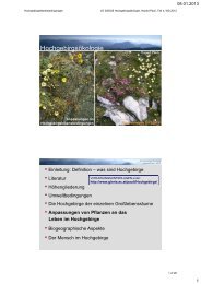
WORKINGSTEP a Marking <strong>the</strong> HSP: This point<br />
should be marked with a small cross cut into <strong>the</strong><br />
solid rock (Fig. 8.3). For sites lacking a solid rock to<br />
mark, metal stakes or o<strong>the</strong>r appropriate markers for<br />
permanent marking should be used. Note that this<br />
mark should persist for decades.<br />
Fig. 8.3 Permanent cross mark at <strong>the</strong> highest summit point<br />
(HSP).<br />
5
351°<br />
<strong>GLORIA</strong> <strong>Field</strong> <strong>Manual</strong> <strong>The</strong> Multi-Summit approach (REVISED DRAFT 2011-06)<br />
8.3.2 Establishing <strong>the</strong> 3m x 3m quadrat clusters and <strong>the</strong> summit area corner points<br />
THE DESIGN<br />
Quadrat clusters: In each <strong>of</strong> <strong>the</strong> four main directions (i.e. <strong>the</strong> true geographic N, E, S & W) a 3m x 3m<br />
quadrat cluster has to be positioned (see Fig. 8.1 and 8.2). Each quadrat cluster consists <strong>of</strong> nine 1m x 1m<br />
quadrats, delineated by a grid <strong>of</strong> flexible measuring tapes (as prepared before field work). <strong>The</strong> lower<br />
boundary <strong>of</strong> each quadrat cluster should lie at <strong>the</strong> 5-m contour line below <strong>the</strong> summit (with a tolerance <strong>of</strong><br />
+/- 0.5 m). <strong>The</strong> lower left or <strong>the</strong> lower right corner point <strong>of</strong> <strong>the</strong> quadrat clusters should be arranged in<br />
<strong>the</strong> main geographic direction (N, E, S, or W) as seen from <strong>the</strong> highest summit point. Thus, <strong>the</strong> quadrat<br />
cluster can ei<strong>the</strong>r lie to <strong>the</strong> right or to <strong>the</strong> left side <strong>of</strong> <strong>the</strong> line indicating <strong>the</strong> main geographic direction<br />
(compare Figs. 8.1 & 8.2) to be decided separately for each cardinal direction depending on <strong>the</strong> particular<br />
terrain and habitat situation.<br />
A deviation from <strong>the</strong> main geographic direction may be necessary if <strong>the</strong> 3m x 3m grid falls on:<br />
(1) too steep terrain to allow safe work or trampling would cause excessive damage, or<br />
(2) it falls on a bare outcrop or boulder field, where available area for plant establishment is negligible.<br />
In <strong>the</strong>se cases, <strong>the</strong> quadrat cluster should be shifted along <strong>the</strong> 5-m contour line to <strong>the</strong> nearest possible<br />
location from <strong>the</strong> original line (i.e. from <strong>the</strong> exact cardinal direction), but <strong>the</strong> 3m x 3m quadrat cluster<br />
always must be within <strong>the</strong> intersection lines (i.e. lines delimiting <strong>the</strong> summit area sections, e.g. <strong>the</strong> exact<br />
geographic SE and SW direction). Wherever possible, summit sites where shifts from <strong>the</strong> exact cardinal<br />
direction are necessary should be avoided. O<strong>the</strong>rwise, always comment on <strong>the</strong> rationale for such shifts.<br />
Summit area-corner points: <strong>The</strong> lower corner points <strong>of</strong><br />
<strong>the</strong> 3m x 3m quadrat clusters also mark <strong>the</strong> lower limit <strong>of</strong><br />
<strong>the</strong> upper summit area (= <strong>the</strong> 5-m summit area).<br />
<strong>The</strong> four lower corner points <strong>of</strong> <strong>the</strong> lower summit area (=<br />
<strong>the</strong> 10-m summit area) lie along <strong>the</strong> straight line connecting<br />
<strong>the</strong> HSP and <strong>the</strong> 5-m corner point (= <strong>the</strong> principal<br />
measurement line), at 10 m elevation below <strong>the</strong> HSP<br />
(compare Fig. 8.2).<br />
<strong>The</strong> suggested working sequence described in this<br />
subchapter must be repeated for each main geographical<br />
direction (N, E, S, & W) and is demonstrated here for <strong>the</strong><br />
N-direction with <strong>the</strong> following workingsteps b-d (compare<br />
with Figs. 8.2, 8.4 & 8.5; see also <strong>the</strong> measurement protocol<br />
sheet (Form 1):<br />
WORKINGSTEP b Determination <strong>of</strong> <strong>the</strong> principal<br />
measurement line (<strong>the</strong> compass direction, <strong>the</strong> vertical<br />
extension, and <strong>the</strong> length <strong>of</strong> this line): i.e. from <strong>the</strong><br />
HSP straight down through a point at <strong>the</strong> 5-m level to <strong>the</strong><br />
endpoint at <strong>the</strong> 10-m level.<br />
Person A stands with a compass and <strong>the</strong> measurement<br />
protocol (Form 1) at <strong>the</strong> HSP and fixes a 50-m<br />
measuring tape at this point. He/she points out <strong>the</strong><br />
geographic N-direction (see Figs. 8.4 & 8.5, and Box<br />
8.1).<br />
Person B begins walking in <strong>the</strong> indicated geographic<br />
N-direction unwinding <strong>the</strong> measuring tape and focusing at<br />
<strong>the</strong> highest summit point with a clinometer. On reaching<br />
an exact horizontal view <strong>of</strong> <strong>the</strong> HSP, a temporary marker<br />
is placed on <strong>the</strong> ground. <strong>The</strong> elevation difference between<br />
<strong>the</strong> marker and <strong>the</strong> HSP equals <strong>the</strong> eye-height (i.e. <strong>the</strong><br />
body length from feet to eyes) <strong>of</strong> person B. This process<br />
is repeated until <strong>the</strong> 5-m point is reached (see Fig. 8.5).<br />
6<br />
Lower boundary<br />
<strong>of</strong> <strong>the</strong><br />
10-m summit area<br />
marked with<br />
a thin string<br />
p5m-N31<br />
(5-m level<br />
below summit)<br />
p-N33<br />
Lower boundary<br />
<strong>of</strong> <strong>the</strong><br />
5-m summit area<br />
marked with<br />
a thin string<br />
(e.g.) 355°<br />
(e.g.) 355°<br />
p10m-N (corner point at <strong>the</strong><br />
10-m level below summit)<br />
Principal measurement line<br />
for <strong>the</strong> North direction<br />
meets one <strong>of</strong> <strong>the</strong> two 5-m corner points <strong>of</strong> <strong>the</strong><br />
quadrat cluster (in this example <strong>the</strong> p5m-N31) and<br />
<strong>the</strong> 10-m point p10m-N<br />
N31 N11<br />
N33 N13<br />
002°<br />
004°<br />
p-N13<br />
p5m-N11<br />
(5-m level<br />
below summit)<br />
Measurement lines<br />
for <strong>the</strong> o<strong>the</strong>r<br />
corner points <strong>of</strong> <strong>the</strong><br />
quadrat cluster<br />
HSP = Highest summit point<br />
(<strong>the</strong> principal reference point)<br />
10 m<br />
Fig. 8.4 Measurement <strong>of</strong> <strong>the</strong> compass<br />
direction from <strong>the</strong> HSP to <strong>the</strong> corner points <strong>of</strong><br />
<strong>the</strong> 3m x 3m quadrat cluster and to <strong>the</strong> 10-m<br />
point. If in our example, <strong>the</strong> magnetic<br />
declination was 5° E, it needs to be corrected<br />
in <strong>the</strong> following way: 355° on <strong>the</strong> compass<br />
(instead <strong>of</strong> 000°/360°) should be sighted on to<br />
give <strong>the</strong> true north for <strong>the</strong> principal<br />
measurement line (see also Box 8.1).<br />
In exceptional cases, deviations from <strong>the</strong> exact<br />
cardinal direction may be necessary if terrain<br />
or habitat is not appropriate for establishing<br />
<strong>the</strong> 3m x 3m plot cluster (compare text in<br />
workingstep b).
<strong>GLORIA</strong> <strong>Field</strong> <strong>Manual</strong> <strong>The</strong> Multi-Summit approach (REVISED DRAFT 2011-06)<br />
When reaching <strong>the</strong> 5-m level, person B decides if <strong>the</strong> location is appropriate for spreading <strong>the</strong><br />
3m x 3m quadrat cluster – if not, ano<strong>the</strong>r location at <strong>the</strong> 5-m level, positioned as close as possible to<br />
<strong>the</strong> exact geographical N-direction, is chosen (if a deviation is necessary, stay, in any case, within <strong>the</strong><br />
area delimited by <strong>the</strong> NW and <strong>the</strong> NE intersections lines which will be established later in workingstep<br />
g).<br />
<strong>The</strong> determined point at <strong>the</strong> 5-m level (this will be ei<strong>the</strong>r point p5m-N11 or p5m-N31, see<br />
workingstep c), will be marked with a small aluminium tube and with some stones to aid <strong>the</strong> fur<strong>the</strong>r<br />
set-up procedure (in workingstep c).<br />
From <strong>the</strong> point at <strong>the</strong> 5-m level, person B continues downward to <strong>the</strong> 10-m level, being guided by<br />
person A. Note that <strong>the</strong> HSP and <strong>the</strong> finally determined position <strong>of</strong> and <strong>the</strong> points at <strong>the</strong> 5-m and <strong>the</strong><br />
10-m levels (e.g. HSP, p5m-N and p10m-N) must lie on <strong>the</strong> same straight line. <strong>The</strong> 10-m point (p10m-<br />
N) will be marked again with a small aluminium tube and with some stones.<br />
Person B tightens <strong>the</strong> 50-m measuring tape (held by person A to ensure that <strong>the</strong> tape is straight<br />
through <strong>the</strong> marked 5-m point), and calls <strong>the</strong> distance read from <strong>the</strong> measuring tape at <strong>the</strong> 10-m point<br />
(see Box 8.3);<br />
person A enters <strong>the</strong> distance value into <strong>the</strong> protocol (Form 1);<br />
person A (standing on <strong>the</strong> HSP) focuses <strong>the</strong> compass on person B (standing on <strong>the</strong> 10-m point) and<br />
takes a reading <strong>of</strong> <strong>the</strong> magnetic compass direction. If person B is not visible to person A, person B<br />
holds up a signal rod perpendicularly;<br />
person A enters <strong>the</strong> magnetic compass direction into <strong>the</strong> protocol sheet (compare Box 8.1).<br />
7
<strong>GLORIA</strong> <strong>Field</strong> <strong>Manual</strong> <strong>The</strong> Multi-Summit approach (REVISED DRAFT 2011-06)<br />
Box 8.1: Compass measurements. <strong>The</strong> magnetic N-direction can deviate considerably from <strong>the</strong><br />
geographic N-direction in some regions and can change in comparatively short periods <strong>of</strong> time.<br />
<strong>The</strong>refore, <strong>the</strong> magnetic declination (i.e. <strong>the</strong> angle between <strong>the</strong> direction <strong>of</strong> <strong>the</strong> geographic North Pole<br />
and <strong>the</strong> magnetic North Pole) has to be identified and indicated on <strong>the</strong> measurement protocol sheet<br />
(Form 1). To fix a point in <strong>the</strong> geographic N-direction, for example, <strong>the</strong> measuring person defines:<br />
(a) <strong>the</strong> magnetic N-direction with <strong>the</strong> compass, (b) corrects it for <strong>the</strong> magnetic declination and<br />
(c) guides <strong>the</strong> person, who fixes <strong>the</strong> points, to <strong>the</strong> corrected geographic N-direction.<br />
This applies to all directions (N, E, S, W as well as to NE, SE, SW, NW; see also below in this box).<br />
However, in any case, only <strong>the</strong> measured magnetic compass directions has to be entered on <strong>the</strong><br />
sampling sheet (From 1), i.e. degrees on <strong>the</strong> 0-360° scale as indicated on <strong>the</strong> compass (see also Fig.<br />
8.4). This is relevant for all numeric indications <strong>of</strong> angles in <strong>the</strong> sampling protocols.<br />
For measuring compass directions, an accuracy <strong>of</strong> +/- 2° can be normally reached with an ordinary<br />
field compass or +/- 1° with a Suunto KB-14/360 compass.<br />
Magnetic declination: <strong>The</strong> magnetic declination should be indicated in degrees (360 ° scale) with its<br />
correct sign (+ or – ) at <strong>the</strong> top <strong>of</strong> <strong>the</strong> measurement protocol (Form 1).<br />
For example, – 6 ( = 6° W = 6° west <strong>of</strong> <strong>the</strong> geogr. North Pole), +20 (= 20° E = 20° east <strong>of</strong> <strong>the</strong> geogr.<br />
North Pole). In sou<strong>the</strong>rn Europe and in <strong>the</strong> European Alps, <strong>the</strong> magnetic declination is currently only<br />
between 1° and 3° E. <strong>The</strong>re are larger declinations, e.g., in N-Sweden (currently 5° E), Caucasus (6°<br />
E), Sou<strong>the</strong>rn Ural (about 13° E), Nor<strong>the</strong>rn Ural (23° E), Central Brooks Range, Alaska (about 25° E) or<br />
on central Ellesmere Island, N-Canada (about 77° W). <strong>The</strong>se examples show that it is important to<br />
consider <strong>the</strong> magnetic declination for establishing <strong>the</strong> permanent plots by using a field compass.<br />
<strong>The</strong> current magnetic declination <strong>of</strong> any place, globally, can be obtained from <strong>the</strong> web site <strong>of</strong> <strong>the</strong> US-<br />
National Geophysical Data Center, Boulder: http://www.ngdc.noaa.gov/geomagmodels/Declination.jsp<br />
<strong>The</strong> magnetic declination must be considered for <strong>the</strong> determination <strong>of</strong> all 4 principal<br />
measurement lines as well as for <strong>the</strong> 4 intersection lines. For example, <strong>the</strong> corrected compass<br />
readings at a given magnetic declination <strong>of</strong> +5 (5° E) are 355° for true/geographic N, 085° for E, 175°<br />
for S, 130° for SE; <strong>the</strong> corresponding values at a magnetic declination <strong>of</strong> –10 (10° W) are: 010° (N),<br />
100° (E), 190° (S), 145° (SE). That means, e.g. for <strong>the</strong> N-direction and a magnetic declination <strong>of</strong> +5:<br />
go towards <strong>the</strong> compass direction 355° to fix <strong>the</strong> principal measurement line and <strong>the</strong> N-cluster (see Fig.<br />
8.4).<br />
Person A with compass (and <strong>the</strong> protocol sheet) stays on <strong>the</strong> HSP<br />
50-m measuring tape<br />
1)<br />
HSP<br />
2)<br />
5.25m<br />
1.75m<br />
1.75m<br />
1.75m<br />
Person B steps downwards with a clinometer (or an<br />
electronic spirit level) and with a<br />
HSP<br />
5.25m<br />
0.25m<br />
determined by a<br />
small measuring<br />
tape<br />
5-m point<br />
Person B with<br />
spirit level and a<br />
small measuring tape<br />
3)<br />
HSP<br />
4)<br />
5-m point<br />
5m<br />
HSP<br />
5m<br />
5-m point<br />
5.25m<br />
1.75m<br />
1.75m<br />
1.75m<br />
5.25m<br />
0.25m<br />
determined by a<br />
small measuring<br />
tape<br />
10-m point<br />
Fig. 8.5 Measurement <strong>of</strong> <strong>the</strong> vertical distances: Person A signals <strong>the</strong> compass direction (see Box 8.1), Person B<br />
(with an eye-height <strong>of</strong>, e.g., 1.75m), measures <strong>the</strong> vertical distance. (1) Three eye-heights down to <strong>the</strong>, e.g., 5.25m<br />
level (depending on <strong>the</strong> actual eye-height <strong>of</strong> person B); (2) Measuring and fixing <strong>of</strong> <strong>the</strong> 5-m point; (3) Three eyeheights<br />
down to <strong>the</strong>, e.g., 10.25m level; (4) Measuring and fixing <strong>of</strong> <strong>the</strong> 10-m point (for tolerances see Box 8.3).<br />
8
<strong>GLORIA</strong> <strong>Field</strong> <strong>Manual</strong> <strong>The</strong> Multi-Summit approach (REVISED DRAFT 2011-06)<br />
WORKINGSTEP c Fixing <strong>the</strong> 3m x 3m quadrat clusters: After <strong>the</strong> principal measurement line with<br />
<strong>the</strong> positions at <strong>the</strong> 5-m and at <strong>the</strong> 10-m levels are determined, <strong>the</strong> 3m x 3m quadrat cluster can be<br />
placed at <strong>the</strong> 5-m level. (Fig. 8.7). This should be made by two persons. Particular care is required at<br />
this step to avoid trampling impacts in <strong>the</strong> plot area (see also Box 8.2).<br />
As indicated above, <strong>the</strong> measured 5-m point is ei<strong>the</strong>r <strong>the</strong> left lower (e.g., p5m-N11) or <strong>the</strong> right<br />
lower corner (e.g., p5m-N31) <strong>of</strong> <strong>the</strong> 3m x 3m grid (dependent on <strong>the</strong> terrain and habitat situation).<br />
Both points (p5m-N11 and p5m-N31) have to be on <strong>the</strong> 5-m level such that <strong>the</strong> left and right<br />
boundaries <strong>of</strong> <strong>the</strong> quadrat cluster are more or less parallel to <strong>the</strong> slope.<br />
<strong>The</strong> corner points <strong>of</strong> each 1m x 1m quadrat <strong>of</strong> <strong>the</strong> grid should be fixed at <strong>the</strong> surface as far as<br />
possible (some corners may stay above <strong>the</strong> surface). This can be done with ordinary 100 mm nails put<br />
through <strong>the</strong> hole <strong>of</strong> <strong>the</strong> blanks (eyelets at <strong>the</strong> crossing points <strong>of</strong> <strong>the</strong> 3m x 3m grid) or through <strong>the</strong> outer<br />
tape material, and/or with stones – a thin wire may be helpful.<br />
In addition, short aluminium tubes should be positioned at <strong>the</strong> corners <strong>of</strong> <strong>the</strong> quadrats as<br />
permanent marks, where applicable. Only <strong>the</strong> upper 1 to 2 cm <strong>of</strong> <strong>the</strong>se tubes should project above <strong>the</strong><br />
surface in order to avoid easy detection by tourists. Where aluminium markers cannot be mounted<br />
(e.g. on solid rock), a small white or yellow point can be painted with durable paint. Permanent<br />
marking with durable material is essential in taller-growing vegetation such as alpine meadows, where<br />
solid rock is absent.<br />
WORKINGSTEP d Measuring <strong>the</strong> distances and <strong>the</strong> magnetic compass directions from <strong>the</strong> HSP<br />
to <strong>the</strong> quadrat cluster corner points: After <strong>the</strong> 3m x 3m grid is fixed, person A, standing directly<br />
above <strong>the</strong> HSP, reads <strong>the</strong> compass directions for <strong>the</strong> 4 outer corner points <strong>of</strong> <strong>the</strong> 3m x 3m quadrat<br />
cluster, assisted by person B, who signals <strong>the</strong> position <strong>of</strong> each point and who measures <strong>the</strong> distance<br />
(see <strong>the</strong> measurement protocol sheet, Form 1 and Box 8.1).<br />
repeat <strong>the</strong> procedure for distance and compass measurements described in workingstep b for<br />
each corner point <strong>of</strong> each quadrat cluster;<br />
after entering <strong>the</strong> 4 distances and <strong>the</strong> 4 compass readings (<strong>of</strong> <strong>the</strong> cluster corner points) into <strong>the</strong><br />
protocol, <strong>the</strong> scribe (person A) should check <strong>the</strong> relevant box in <strong>the</strong> measurement protocol (Form 1) to<br />
indicate whe<strong>the</strong>r, e.g., point p5m-N11 or point p5m-N31 lies on <strong>the</strong> principal measurement line.<br />
Note: always write <strong>the</strong> magnetic compass directions (i.e. <strong>the</strong> degree as indicated on <strong>the</strong> compass).<br />
Box 8.2: Trampling impacts by <strong>the</strong> investigators. Trampling impacts during <strong>the</strong> set-up and<br />
removal <strong>of</strong> plot grids as well as during <strong>the</strong> sampling should be minimised. Particular care must be<br />
taken, e.g., in some lichen- or bryophyte-dominated communities, snowbed and tall meadow vegetation<br />
or in unstable scree fields.<br />
Sleeping pads, such as those commonly used by campers, may be useful during sampling where terrain<br />
is appropriate.<br />
Box 8.3:<br />
Measurement accuracy and tolerances.<br />
• Distances are to be measured to <strong>the</strong> nearest 1 cm (e.g. 13.63 m). Although this is "over-accurate" on<br />
most surfaces and with long distances, <strong>the</strong>re is no reason to round up to lower resolutions.<br />
Distances are always measured in <strong>the</strong> shortest straight line from <strong>the</strong><br />
HSP to a corner point with <strong>the</strong> measurement tape tightened.<br />
<strong>The</strong>refore, all measurement distances are surface distances<br />
and not top view distances.<br />
• Horizontal angles measured with <strong>the</strong> compass are to be indicated with an accuracy <strong>of</strong> +/- 2°. This<br />
can be reached with an ordinary field compass.<br />
• Vertical angles, i.e <strong>the</strong> average slope <strong>of</strong> <strong>the</strong> area <strong>of</strong> <strong>the</strong> 1m x 1m plot, as measured with an<br />
electronic spirit level or a clinometer should be indicated in degrees, using <strong>the</strong> 360° scale.<br />
• <strong>The</strong> corner points <strong>of</strong> <strong>the</strong> 5-m and <strong>the</strong> 10-m summit area are to be set up with a tolerance <strong>of</strong> +/- 0.5<br />
vertical metres.<br />
9
<strong>GLORIA</strong> <strong>Field</strong> <strong>Manual</strong> <strong>The</strong> Multi-Summit approach (REVISED DRAFT 2011-06)<br />
Box 8.4:<br />
Modification <strong>of</strong> <strong>the</strong> sampling design for flat summit areas.<br />
Some mountain ranges may be dominated by flat, plateau-shaped summits, and "moderately" shaped<br />
summits may be difficult to find. <strong>The</strong> sampling area at flat summits would be much larger when setting<br />
<strong>the</strong> 3m x 3m grid at <strong>the</strong> 5-m level below <strong>the</strong> highest summit point and <strong>the</strong> lower corner points <strong>of</strong> <strong>the</strong><br />
10-m summit area at <strong>the</strong> 10-m level. This would significantly leng<strong>the</strong>n <strong>the</strong> measurement work for<br />
setting <strong>the</strong> plots and <strong>the</strong> work for summit area sampling. Fur<strong>the</strong>rmore, <strong>the</strong>se large summits areas are<br />
not ideal for summit comparisons.<br />
Flat plateau summits should be avoided whenever possible, but in <strong>the</strong> absence <strong>of</strong> alternative sites, <strong>the</strong><br />
following modifications to <strong>the</strong> general protocol should be applied.<br />
As a rule <strong>of</strong> thumb, we suggest: if <strong>the</strong> 5-m level is not reached within 50-m surface distance from <strong>the</strong><br />
highest summit point (HSP), establish <strong>the</strong> 3m x 3m grid at <strong>the</strong> 50-m distance point. <strong>The</strong>refore, in <strong>the</strong>se<br />
flat terrain situations, <strong>the</strong> distance measurement with <strong>the</strong> measuring tape should be done immediately<br />
after measuring <strong>the</strong> vertical distances and before <strong>the</strong> 3m x 3m grid is established.<br />
Similarly, if <strong>the</strong> 10-m level is not reached within 100 m, put <strong>the</strong> 10-m point at <strong>the</strong> 100-m distance<br />
point.<br />
In cases where <strong>the</strong> lower boundary <strong>of</strong> <strong>the</strong> 3m x 3m grid has to be established above <strong>the</strong> 5-m level at <strong>the</strong><br />
50-m surface distance from <strong>the</strong> HSP, <strong>the</strong> 10-m point has to be established at <strong>the</strong> actual 10-m level if<br />
this can be reached within a 100-m surface distance from <strong>the</strong> HSP; this means more than 5 m in<br />
elevation below <strong>the</strong> 3m x 3m grid.<br />
8.3.3 Establishing <strong>the</strong> boundary lines <strong>of</strong> <strong>the</strong> summit areas and <strong>the</strong> summit area sections<br />
THE DESIGN<br />
Summit areas: A string around <strong>the</strong> summit, connecting <strong>the</strong> 8 corner points at <strong>the</strong> 5-m level, delimits <strong>the</strong><br />
upper summit area (= 5-m summit area). <strong>The</strong> corner points at <strong>the</strong> 5-m level will be connected around <strong>the</strong><br />
summit in straight surface lines. Thus, <strong>the</strong> 5-m summit area reaches <strong>the</strong> 5-m level below <strong>the</strong> highest<br />
summit point only at <strong>the</strong> 4 clusters, and lies usually above <strong>the</strong> 5-m contour line between <strong>the</strong> clusters<br />
(compare Fig. 8.1 and 8.2). This helps to keep <strong>the</strong> area to a reasonable size – particularly at elongated<br />
summits. Fur<strong>the</strong>rmore, it simplifies <strong>the</strong> procedure, because an exact marking along <strong>the</strong> 5-m contour line<br />
would multiply <strong>the</strong> time required, but without enhancing <strong>the</strong> quality <strong>of</strong> <strong>the</strong> data substantially.<br />
<strong>The</strong> corner points at <strong>the</strong> 10-m level, connected in <strong>the</strong> same manner, mark <strong>the</strong> lower limit <strong>of</strong> <strong>the</strong> lower<br />
summit area (= 10-m summit area), which forms a zone around <strong>the</strong> 5-m summit area. <strong>The</strong> 10-m summit<br />
area does not include (or overlap with) <strong>the</strong> 5-m summit area (see Fig. 8.6, compare Figs. 8.1 & 8.2).<br />
<strong>The</strong> distances between <strong>the</strong> corner points <strong>of</strong> <strong>the</strong> 5-m summit area and between <strong>the</strong> corner points <strong>of</strong> <strong>the</strong> 10-<br />
m summit area will not be measured.<br />
Summit area sections: Each <strong>of</strong> <strong>the</strong> two summit areas is to be divided into four summit area sections by<br />
straight lines running from <strong>the</strong> HSP to <strong>the</strong> summit area boundary lines, in <strong>the</strong> NE, SE, SW and NW<br />
directions (four intersection lines; see Fig. 8.6). <strong>The</strong> exact geographic direction is to be determined and<br />
<strong>the</strong> distance from <strong>the</strong> HSP to <strong>the</strong> points, where <strong>the</strong> two summit area boundary lines cross with <strong>the</strong><br />
intersection lines, is to be measured.<br />
WORKINGSTEP e Establishing <strong>the</strong> boundary line <strong>of</strong> <strong>the</strong> 5-m summit area: This must be done by<br />
at least two persons, but three are <strong>of</strong>ten recommendable in a more rugged terrain.<br />
Person A starts from one <strong>of</strong> <strong>the</strong> lower corners <strong>of</strong> a 3m x 3m quadrat cluster (e.g. <strong>the</strong> lower left <strong>of</strong> <strong>the</strong><br />
N-quadrat cluster: at point p5m-N11) where a string is fixed.<br />
Person A <strong>the</strong>n walks with <strong>the</strong> string to point p5m-E31 <strong>of</strong> <strong>the</strong> E-quadrat cluster. When this point is<br />
reached, <strong>the</strong> string should be tightened and fixed at this point to connect <strong>the</strong> two points (p5m-N11 and<br />
p5m-E31) in <strong>the</strong> shortest straight line possible.<br />
Person B helps person A to keep <strong>the</strong> straight line.<br />
This procedure continues by fixing <strong>the</strong> string also at p5m-E11 <strong>of</strong> <strong>the</strong> E-quadrat cluster and by<br />
heading fur<strong>the</strong>r to <strong>the</strong> S-quadrat cluster (an so on), where <strong>the</strong> same work is repeated until <strong>the</strong> N-<br />
quadrat cluster is reached again at its lower right corner (p5m-N31).<br />
10
<strong>GLORIA</strong> <strong>Field</strong> <strong>Manual</strong> <strong>The</strong> Multi-Summit approach (REVISED DRAFT 2011-06)<br />
WORKINGSTEP f Establishing <strong>the</strong> boundary line <strong>of</strong> <strong>the</strong> 10-m summit area: In <strong>the</strong> same manner,<br />
<strong>the</strong> 4 corner points at <strong>the</strong> 10-m level (from p10m-N to p10m-E, p10m-S, p10m-W, and back to p10m-<br />
N) will be connected with straight strings.<br />
10-m contour line<br />
N-10m-SA<br />
5-m summit area<br />
NW<br />
5-m contour line<br />
NE<br />
10-m summit area<br />
N-5m-SA<br />
10 m<br />
W-10m-SA<br />
W-5m-SA<br />
S-5m-SA<br />
E-5m-SA<br />
E-10m-SA<br />
NW<br />
N-10m-SA<br />
NE<br />
10-m contour line<br />
5-m contour line<br />
SW<br />
S-10m-SA<br />
W<br />
W-10m-SA<br />
W-5m-SA<br />
N-5m-SA<br />
S-5m-SA<br />
E-5m-SA<br />
E-10m-SA<br />
SE<br />
Two examples for a summit area<br />
with <strong>the</strong> summit area sections:<br />
above left: <strong>the</strong> “ideal” case from<br />
an evenly shaped summit;<br />
right: a more common situation.<br />
Principal<br />
measurement<br />
line<br />
SW<br />
S-10m-SA<br />
SE<br />
Fig. 8.6 Eight summit area sections (= 4 subdivisions <strong>of</strong> <strong>the</strong> 5-m summit area and 4 subdivisions <strong>of</strong> <strong>the</strong> 10-m<br />
summit area). <strong>The</strong> area <strong>of</strong> <strong>the</strong> sections depends <strong>of</strong> <strong>the</strong> shape <strong>of</strong> <strong>the</strong> summit. Thus, it is usually different among <strong>the</strong><br />
main directions (see <strong>the</strong> right sketch). <strong>The</strong> sections <strong>of</strong> <strong>the</strong> 10-m summit area are usually larger. <strong>The</strong> intersection<br />
lines always point from <strong>the</strong> HSP exactly to <strong>the</strong> geographic NE, SE, SW, NW directions, respectively.<br />
In contrast, <strong>the</strong> principal measurement lines (from <strong>the</strong> HSP to N, E, S, W, respectively) may, in exceptional cases,<br />
deviate from <strong>the</strong>ir geographic direction, dependent on <strong>the</strong> terrain and habitat situation (e.g. see W-direction in <strong>the</strong><br />
right sketch; see also workingstep b in subchapter 8.3.2).<br />
WORKINGSTEP g Dividing <strong>the</strong> summit areas into sections:<br />
Person A takes position at <strong>the</strong> HSP and indicates <strong>the</strong> appropriate compass bearing that runs in<br />
between two neighbouring corner points, i.e. NE for <strong>the</strong> corner points p10m-N and p10m-E. <strong>The</strong> same<br />
correction for magnetic declination should be taken into account as used for setting up <strong>the</strong> summit area<br />
corner points (see Fig. 8.6 and Box 8.1).<br />
After attaching one end <strong>of</strong> a roll <strong>of</strong> string to <strong>the</strong> HSP, Person B follows <strong>the</strong> direction indicated<br />
by person A. Where <strong>the</strong> tightened string crosses <strong>the</strong> boundaries <strong>of</strong> <strong>the</strong> summits areas (e.g. pNE-5 and<br />
pNE-10), a marker is placed (e.g. a small aluminium tube and some stones). <strong>The</strong> procedure is repeated<br />
for <strong>the</strong> remaining three directions. This results in a N, E, S, & W section <strong>of</strong> <strong>the</strong> 5-m summit area as<br />
well as <strong>of</strong> <strong>the</strong> 10-m summit area (see Fig. 8.6).<br />
Finally, person A takes a compass reading from <strong>the</strong> HSP to <strong>the</strong> marked points (consider <strong>the</strong><br />
magnetic declination, see Box 8.1), and person B, supported by person A, measures <strong>the</strong> surface<br />
distance between <strong>the</strong> HSP and <strong>the</strong> two marked crossing points along each <strong>of</strong> <strong>the</strong> 4 intersection lines<br />
(e.g., from <strong>the</strong> HSP to pNE-5 and from HSP to pNE-10).<br />
On completing this step, <strong>the</strong> summit areas and quadrats are ready for recording. Before starting <strong>the</strong><br />
recording, check that all entries have been completed on <strong>the</strong> measurement protocol (Form 1). <strong>The</strong><br />
"checkboxes" on Form 1 for photo documentation <strong>of</strong> <strong>the</strong> 1m x 1m quadrats and <strong>the</strong> corner points (see<br />
chapter 8.4.4 with <strong>the</strong> workingsteps o to r and t) are usually filled later on by <strong>the</strong> person responsible<br />
11
<strong>GLORIA</strong> <strong>Field</strong> <strong>Manual</strong> <strong>The</strong> Multi-Summit approach (REVISED DRAFT 2011-06)<br />
for <strong>the</strong> photo documentation. For measurement tolerances, see Box 8.3; for <strong>the</strong> reasoning behind <strong>the</strong>se<br />
measurements, see Box 8.10.<br />
If all measurements were made correctly, <strong>the</strong> size <strong>of</strong> <strong>the</strong> summit area sections is calculated<br />
automatically by <strong>the</strong> <strong>GLORIA</strong> data input tool. Sketches <strong>of</strong> <strong>the</strong> actual summit design will be produced<br />
by <strong>the</strong> <strong>GLORIA</strong> co-ordination group once data are uploaded to <strong>the</strong> central <strong>GLORIA</strong> data base.<br />
<strong>The</strong>refore, it is crucial that <strong>the</strong> measurement protocol (Form 1) is complete in <strong>the</strong> field, without any<br />
missing measurements.<br />
8.4 <strong>The</strong> required recording procedures<br />
This chapter describes all recording methods and working steps that are considered as obligatory and<br />
standard components <strong>of</strong> <strong>the</strong> Multi-Summit approach, applied by all teams in all target regions.<br />
8.4.1 Recording in <strong>the</strong> 1m x 1m quadrats<br />
Each 3m x 3m quadrat cluster consists <strong>of</strong> nine 1m x 1m quadrats, as set out by <strong>the</strong> grid <strong>of</strong> flexible<br />
measuring tapes. Vegetation is recorded in <strong>the</strong> four corner quadrats only (see Fig. 8.7), as <strong>the</strong> o<strong>the</strong>rs may<br />
become damaged through trampling by <strong>the</strong> investigators during recording. This yields vegetation data for<br />
16 quadrats <strong>of</strong> 1m x 1m per summit, defined as <strong>the</strong> 16-quadrat area.<br />
In each <strong>of</strong> <strong>the</strong> 16 1m x 1m quadrats, <strong>the</strong> top cover <strong>of</strong> surface types (vascular plant cover, solid rock,<br />
scree, etc.) and species cover <strong>of</strong> each vascular plant species are recorded. <strong>The</strong> aim is to provide a baseline<br />
for detecting changes in species composition and in vegetation cover.<br />
Two methods <strong>of</strong> cover recording are to be applied for <strong>the</strong> required <strong>GLORIA</strong> standard:<br />
1.visual cover estimation (to be done first) and<br />
2. pointing with a grid frame (after completion <strong>of</strong> <strong>the</strong> visual cover estimation).<br />
Note: Frequency counting in 1m²-quadrats is now considered as an optional method that may be applied<br />
supplementary.<br />
8.4.1.1 Visual cover estimation in 1m x 1m quadrats<br />
Both percentage cover <strong>of</strong> surface types and percentage cover <strong>of</strong> each vascular plant species are to be<br />
recorded by means <strong>of</strong> visual cover estimation. This is an effective method for recording all species<br />
occurring within <strong>the</strong> plot, including those with cover values <strong>of</strong> less than one percent. For general<br />
considerations on cover recording in 1-m² quadrats see Box 8.5.<br />
For <strong>the</strong> sampling sheet see Form 2.<br />
WORKINGSTEP h Recording <strong>of</strong> habitat characteristics:<br />
In each quadrat, <strong>the</strong> top cover <strong>of</strong> each surface type is visually estimated. Top cover is <strong>the</strong> vertical<br />
projection (perpendicular to <strong>the</strong> slope angle) <strong>of</strong> each surface type and adds up to 100%, whilst cover,<br />
or species cover (see below) takes into account overlaps between layers. In closed vegetation <strong>the</strong> latter<br />
is usually > than 100% (GREIG-SMITH 1983).<br />
Surface types and <strong>the</strong> estimation <strong>of</strong> <strong>the</strong>ir top cover (%):<br />
- vascular plants: top cover <strong>of</strong> vascular plant vegetation;<br />
- solid rock: rock outcrops – rock which is fixed in <strong>the</strong> ground and does not move even slightly (e.g.<br />
when pushing with <strong>the</strong> boot); large boulders which do not move should be considered as solid rock<br />
and not as scree (if you are in doubt whe<strong>the</strong>r a boulder is scree or solid rock, add it to solid rock);<br />
- scree: debris material – this includes unstable or stable scree fields, as well as single stones <strong>of</strong><br />
various size, lying on <strong>the</strong> surface or +/- fixed in <strong>the</strong> soil substrate; <strong>the</strong> grain size is bigger than <strong>the</strong><br />
sand fraction (as opposed to bare ground);<br />
- lichens on soil: lichens growing on soil not covered by vascular plants;<br />
12
<strong>GLORIA</strong> <strong>Field</strong> <strong>Manual</strong> <strong>The</strong> Multi-Summit approach (REVISED DRAFT 2011-06)<br />
- bryophytes on soil: bryophytes growing on soil not covered by vascular plants;<br />
- bare ground: open soil (organic or mineral), i.e. <strong>the</strong> earthy or sandy surface which is not covered<br />
by plants;<br />
- litter: dead plant material.<br />
Each <strong>of</strong> <strong>the</strong>se types represents a fraction <strong>of</strong> <strong>the</strong> 1m²-area; this means that <strong>the</strong> sum <strong>of</strong> <strong>the</strong> top cover<br />
values <strong>of</strong> all present surface types adds up to 100%.<br />
Subtypes estimated for top cover:<br />
- lichens below vascular plants: lichens growing below <strong>the</strong> vascular plant layer;<br />
- bryophytes below vascular plants: bryophytes growing below <strong>the</strong> vascular plant layer;<br />
- lichens on solid rock: epilithic lichens on rock outcrops;<br />
- bryophytes on solid rock: bryophytes on rock growing in micro-fissures where soil material is not<br />
visible (as opposed to bryophytes on soil);<br />
- lichens on scree: epilithic lichens growing on scree or on single stones;<br />
- bryophytes on scree: bryophytes on scree or stones growing in micro-fissures where soil is not<br />
visible.<br />
Each <strong>of</strong> <strong>the</strong>se subtypes represents a fraction <strong>of</strong> one <strong>of</strong> <strong>the</strong> following surface types: vascular plants,<br />
solid rock, or scree. <strong>The</strong> subtype cover is to be estimated as a percentage <strong>of</strong> <strong>the</strong> surface type cover. For<br />
example, in a quadrat where 40% is covered by solid rock and half <strong>of</strong> <strong>the</strong> rock is covered by lichens,<br />
enter <strong>the</strong> value 50% for <strong>the</strong> subtype "lichens on solid rock" into <strong>the</strong> sampling form (and not 20%,<br />
which would be <strong>the</strong> percentage referring to <strong>the</strong> whole quadrat).<br />
<strong>The</strong> average aspect <strong>of</strong> <strong>the</strong> quadrat (in <strong>the</strong> categories N, NE, E, SE, S, SW, W, or NW) is<br />
recorded by using a compass. For <strong>the</strong> average slope (in degrees, 360° scale) use a clinometer.<br />
WORKINGSTEP i Recording <strong>of</strong> <strong>the</strong> species composition and cover:<br />
<strong>The</strong> cover value <strong>of</strong> each vascular plant species is visually determined. <strong>The</strong> recording <strong>of</strong><br />
bryophytes and lichens on <strong>the</strong> species level is optional. Cover values are estimated by using a<br />
percentage scale relative to <strong>the</strong> total quadrat area <strong>of</strong> 1m². <strong>The</strong> percentage cover should be estimated as<br />
precisely as possible for monitoring purposes, particularly for <strong>the</strong> less abundant species; to calibrate<br />
yourself, use transparent templates that show different area sizes (see Figs. AI.3a/b in Annex I <strong>of</strong> <strong>the</strong><br />
<strong>Field</strong> <strong>Manual</strong>).<br />
Please note that <strong>the</strong> total cover sum <strong>of</strong> all vascular plant species may exceed <strong>the</strong> top cover estimated<br />
for vascular plants in workingstep h due to overlapping vegetation layers.<br />
See Box 8.5 for general considerations on this method. For considerations concerning <strong>the</strong><br />
determination <strong>of</strong> vascular plants with regard to <strong>the</strong> taxonomic level and concerning cryptogam species<br />
see Box 8.6.<br />
Box 8.5:<br />
Vegetation records in <strong>the</strong> 1m x 1m quadrats – general considerations.<br />
Top cover <strong>of</strong> surface types<br />
<strong>The</strong> surface types defined under workingstep h characterise <strong>the</strong> habitat situation <strong>of</strong> <strong>the</strong> plot, based on<br />
easily distinguishable surface patterns.<br />
Species cover sampling<br />
A key advantage <strong>of</strong> cover as a measure <strong>of</strong> vegetation or <strong>of</strong> a species occurrence is that it does not<br />
require <strong>the</strong> identification <strong>of</strong> <strong>the</strong> individual (as density does), yet it is an easily visualized and intuitive<br />
measure and, compared to density and frequency, it is <strong>the</strong> most directly related to biomass (Elzinga et<br />
al. 1998). <strong>The</strong> main general disadvantage <strong>of</strong> cover measures is that cover might fluctuate over <strong>the</strong><br />
course <strong>of</strong> a growing season. This, however, is <strong>of</strong> inferior relevance in most types <strong>of</strong> high mountain<br />
vegetation which are predominantly composed <strong>of</strong> long-lived and slow-growing species. Recording<br />
during <strong>the</strong> peak growing season (at least outside <strong>of</strong> humid tropical regions) will potentially capture <strong>the</strong><br />
13
<strong>GLORIA</strong> <strong>Field</strong> <strong>Manual</strong> <strong>The</strong> Multi-Summit approach (REVISED DRAFT 2011-06)<br />
large majority <strong>of</strong> species and species cover <strong>of</strong> most species is not expected to markedly change until<br />
<strong>the</strong> end <strong>of</strong> <strong>the</strong> season.<br />
Visual cover estimation<br />
<strong>The</strong> visual estimation is <strong>the</strong> most effective method for detecting all vascular plant species. Particularly<br />
in low-stature high mountain vegetation it is easily applicable and works fairly rapid.<br />
In <strong>GLORIA</strong> permanent quadrats, species cover should be estimated as precisely as possible on <strong>the</strong><br />
percentage scale. Cover-abundance scales used for vegetation relevés (e.g. BRAUN-BLANQUET, 1964)<br />
are too coarse for this purpose. For example, low cover values <strong>of</strong> species (< 1%), which are <strong>of</strong>ten put<br />
into one class, still show large differences, in alpine environments in particular. Even adult or<br />
flowering individuals <strong>of</strong> a species can cover less than 0.01% <strong>of</strong> a quadrat (i.e. < 1 cm²), whereas o<strong>the</strong>r<br />
species with <strong>the</strong> same number <strong>of</strong> individuals may cover 100 times more or even larger areas.<br />
<strong>The</strong> visual estimation <strong>of</strong> species percentage cover involves a degree <strong>of</strong> inaccuracy and may be<br />
criticised as being too subjective for long-term monitoring where fieldworkers change over time. At<br />
<strong>GLORIA</strong> quadrats, however, <strong>the</strong> scale on <strong>the</strong> measuring tapes delimiting <strong>the</strong> plot and <strong>the</strong> unvarying<br />
size <strong>of</strong> 1m² increase <strong>the</strong> precision <strong>of</strong> <strong>the</strong> percentage cover estimation. A particular area covered by a<br />
species can easily be transformed into percentage cover values (e.g. an area <strong>of</strong> 10 x 10 cm equals 1%, 1<br />
x 1 cm equals 0.01%). Transparent templates, showing <strong>the</strong> area <strong>of</strong> 1%, 0.5% 0.1% etc., facilitate <strong>the</strong><br />
estimation process and should be used particularly when starting to make records <strong>of</strong> a new vegetation<br />
type (see Figs. AI.3a/b in Annex I <strong>of</strong> <strong>the</strong> <strong>Field</strong> <strong>Manual</strong>). Species cover estimation for broad-leaved<br />
species and cushions works well, especially in open vegetation, while <strong>the</strong> estimation <strong>of</strong> graminaceous<br />
species and <strong>of</strong> species in multi-layered and dense vegetation requires experience. Working in observer<br />
pairs is recommended, as it was found that this reduces <strong>the</strong> proportion <strong>of</strong> overlooked species (VITTOZ<br />
& GUISAN 2007).<br />
<strong>The</strong> reproducibility <strong>of</strong> a method among different observers is <strong>of</strong> importance for monitoring changes in<br />
species composition and cover. Previous studies showed that changes less than circa 20% are usually<br />
attributable to variation between observers (SYKES et al. 1983; KENNEDY & ADDISON 1987; NAGY et<br />
al. 2002); <strong>the</strong>refore only changes larger than that may be attributed to causal factors. For comparisons<br />
<strong>of</strong> monitoring data, however, it is crucial to know if we have to deal with a systematic or with a<br />
random observer error. Systematic errors arise when a particular person is notoriously over- or underestimating<br />
<strong>the</strong> cover <strong>of</strong> species, i.e. an error that is invariant within an observer, but varies between<br />
observers, as opposed to random errors deriving from one and <strong>the</strong> same observer from one estimate to<br />
<strong>the</strong> next. Recent field trials with 14 persons independently recording <strong>the</strong> same <strong>GLORIA</strong> test plots <strong>of</strong> 1<br />
m² in different types <strong>of</strong> alpine vegetation showed that random errors contribute by far more to <strong>the</strong><br />
overall observer variance (~ 95%) than systematic errors (~ 5%), (GOTTFRIED et al. 2011, in prep.).<br />
This suggests that different plots can be considered as being sampled independently, irrespective<br />
whe<strong>the</strong>r being recorded by <strong>the</strong> same or by different observers. Consequently, a continuity <strong>of</strong> <strong>the</strong><br />
observing person across two or more monitoring cycles is <strong>of</strong> minor importance. Fur<strong>the</strong>r, <strong>the</strong> power for<br />
change detection much depends on <strong>the</strong> number <strong>of</strong> samples.<br />
Cover recording with point-framing<br />
Point-framing (LEVY & MADDEN 1933) is considered to be an objective method for measuring species<br />
cover (Everson et al. 1990). A key disadvantage <strong>of</strong> point-framing, however, is that points rarely<br />
intersect <strong>the</strong> less common species (compare SORRELLS & GLENN 1991; MEESE & TOMICH 1992;<br />
BRAKENHIELM & LIU 1995; VANHA-MAJAMAA et al. 2000). This is intuitively obvious: a species with<br />
1% cover would likely only be intercepted once or twice (or not at all) in a sample <strong>of</strong> 100 points. A<br />
comparison <strong>of</strong> point-framing and visual cover estimation in open low-stature subnival vegetation<br />
(vegetation top cover <strong>of</strong> ~ 50% or less) showed that, at cover values above 0.7%, <strong>the</strong> two methods did<br />
not show significantly different results (FRIEDMANN et al. 2011); consensus, however, may decrease in<br />
14
<strong>GLORIA</strong> <strong>Field</strong> <strong>Manual</strong> <strong>The</strong> Multi-Summit approach (REVISED DRAFT 2011-06)<br />
more complex vegetation. Yet, point-framing missed 40% <strong>of</strong> <strong>the</strong> species found by visual cover<br />
recording (FRIEDMANN et al. 2011). Point-framing, never<strong>the</strong>less, is considered to yield reliable<br />
reference cover value for <strong>the</strong> more common species and is a rapid method when just making 100<br />
points.<br />
Box 8.6:<br />
<strong>The</strong> required level <strong>of</strong> taxonomic identification and herbarium material.<br />
Vascular plants should be identified in <strong>the</strong> field as accurately as possible and at least to <strong>the</strong> species<br />
level (or in taxonomically complex cases to <strong>the</strong> species aggregate level); if applicable and possible<br />
plants should be identified down to <strong>the</strong> subspecies or variety level.<br />
Given <strong>the</strong> long-term perspective <strong>of</strong> alpine plant monitoring (surveillance) with 5 to 10 year intervals <strong>of</strong><br />
resurvey, it is advisable to make herbarium vouchers for each <strong>of</strong> your species found within <strong>the</strong> four<br />
summit sites <strong>of</strong> your target region. In any cases <strong>of</strong> doubtful identification, a herbarium documentation<br />
is crucial. Herbarium material, archived as a <strong>GLORIA</strong> collection at <strong>the</strong> respective institution, would<br />
facilitate <strong>the</strong> work <strong>of</strong> future field teams and reduces possible observer errors caused by<br />
misidentification. Use standard herbarium labelling with accurate geographic indications.<br />
Please strictly avoid collecting plant specimen from inside <strong>the</strong> 1m x 1m permanent plots or even from<br />
inside <strong>the</strong> 3m x 3m quadrat clusters.<br />
Cryptogam species. <strong>The</strong> identification <strong>of</strong> bryophytes and lichens would be desirable to <strong>the</strong> species<br />
level. However, as identification <strong>of</strong> some cryptogams may not be possible in <strong>the</strong> field, and <strong>the</strong><br />
estimation <strong>of</strong> individual species cover values is very time-consuming, <strong>the</strong> sampling <strong>of</strong> bryophytes and<br />
lichens is not obligatory for <strong>the</strong> standard data set <strong>of</strong> <strong>the</strong> Multi-Summit approach.<br />
In some mountain regions, where cryptogam species contribute substantially to <strong>the</strong> phytomass, <strong>the</strong>ir<br />
recording on a species level is recommended if experts are available. In <strong>the</strong> case that somebody decides<br />
to record cryptogam species, he/she should be aware <strong>of</strong> a significant extension <strong>of</strong> <strong>the</strong> field work period<br />
and <strong>of</strong> <strong>the</strong> risk <strong>of</strong> additional trampling impacts caused by <strong>the</strong> investigators.<br />
Boundary line <strong>of</strong> <strong>the</strong><br />
5-m summit area<br />
S31<br />
S11<br />
S13<br />
S33<br />
Towards <strong>the</strong> summit<br />
p-S13<br />
(Row 3)<br />
(Row 2)<br />
(Row 1)<br />
(Column 3)<br />
(Column 2)<br />
(Column 1)<br />
S13<br />
Not to be sampled<br />
Not to be sampled<br />
(S12) (S22) (S32)<br />
S11<br />
(S23)<br />
(S21)<br />
S33<br />
S31<br />
p-S33<br />
3m<br />
Towards <strong>the</strong> summit<br />
p5m-S11<br />
p5m-S31<br />
Fig. 8.7 <strong>The</strong> 3m x 3m quadrat cluster. Left, example from <strong>the</strong> NE-Alps (2250m), quadrat cluster in <strong>the</strong> S-direction;<br />
right, scheme <strong>of</strong> <strong>the</strong> quadrat cluster with <strong>the</strong> quadrat codes and numbers <strong>of</strong> <strong>the</strong> measurement points (corner points).<br />
<strong>The</strong> quadrat codes consist <strong>of</strong> 3 digits: 1st digit: a letter which denotes to <strong>the</strong> main compass direction, 2nd digit: a<br />
number referring to <strong>the</strong> column <strong>of</strong> <strong>the</strong> cluster numbered from left to right (left and right always defined in <strong>the</strong> sight<br />
to <strong>the</strong> summit), 3rd digit: a number referring to <strong>the</strong> row <strong>of</strong> <strong>the</strong> cluster numbered from bottom to top (in <strong>the</strong> sight to<br />
<strong>the</strong> summit). For example, S31 is <strong>the</strong> quadrat in <strong>the</strong> sou<strong>the</strong>rn quadrat cluster positioned in <strong>the</strong> third column (i.e. <strong>the</strong><br />
right side) and in <strong>the</strong> first row (i.e. <strong>the</strong> lower side; see also Box 9.2 in <strong>the</strong> <strong>Field</strong> <strong>Manual</strong> for coding).<br />
15
<strong>GLORIA</strong> <strong>Field</strong> <strong>Manual</strong> <strong>The</strong> Multi-Summit approach (REVISED DRAFT 2011-06)<br />
8.4.1.2 Pointing with a grid frame in 1m x 1m quadrats<br />
In each <strong>of</strong> <strong>the</strong> 16 1m x 1m quadrats (see Fig. 8.7), a point intercept method (point-framing) is applied,<br />
using a grid frame <strong>of</strong> 1m x 1m inner width and 100 crosshair points distributed regularly over <strong>the</strong> plot.<br />
<strong>The</strong> aim is to provide a baseline for detecting changes in <strong>the</strong> cover <strong>of</strong> <strong>the</strong> more common species. See also<br />
Box 8.5 for general considerations on cover recording.<br />
<strong>The</strong> sampling sheet is combined with that for visual cover estimation so that <strong>the</strong>re is no need to list <strong>the</strong><br />
species names again (see Form 2).<br />
Please note that point recording must be made after <strong>the</strong> visual cover estimation to avoid any bias when<br />
estimating <strong>the</strong> percentage cover.<br />
For <strong>the</strong> construction <strong>of</strong> <strong>the</strong> grid frame see Fig. 8.8 (note that <strong>the</strong> arrangement <strong>of</strong> strings deviates from <strong>the</strong><br />
design used for frequency counts, <strong>the</strong> latter now being considered as an optional supplementary method).<br />
WORKINGSTEP j Pointing <strong>of</strong> surface types and<br />
vascular plant species: Use a wooden (or aluminium)<br />
grid frame <strong>of</strong> 1m x 1m inner width and 10 strings<br />
tightened in each direction. <strong>The</strong> resulting 100 crosshair<br />
intersections (see Fig. 8.8 for construction) will be used<br />
for <strong>the</strong> point recording.<br />
Mount <strong>the</strong> frame above <strong>the</strong> plot so that <strong>the</strong> inner<br />
edges optimally lie above <strong>the</strong> measuring tapes that<br />
delimit <strong>the</strong> plot.<br />
Use a sampling pin <strong>of</strong> 2mm diameter (e.g. a thin<br />
knitting needle) for <strong>the</strong> point recording.<br />
Lower <strong>the</strong> pin perpendicularly to <strong>the</strong> slope (i.e.<br />
perpendicularly to <strong>the</strong> plane <strong>of</strong> <strong>the</strong> grid frame) at each<br />
crosshair intersection.<br />
Hits are tallied (noted with a stroke) when <strong>the</strong> pin<br />
makes contact with a plant or with <strong>the</strong> ground:<br />
- When you hit a vascular plant, make a stroke in <strong>the</strong><br />
respective line on your sampling sheet.<br />
- Continue to lower down <strong>the</strong> pin if <strong>the</strong>re is a second<br />
vascular plant layer below; also make a stroke for any<br />
Fig. 8.8. Grid frame <strong>of</strong> 1m x 1m (inner width)<br />
for point recording at 100 crosshair<br />
intersections; 5 cm string distance from inner<br />
margin, 10 cm distance between strings.<br />
o<strong>the</strong>r vascular plant species that are hit below <strong>the</strong> uppermost one. However, never note <strong>the</strong> surface at<br />
points where you hit a vascular plant.<br />
- Where no vascular plant is present, make a stroke for <strong>the</strong> surface type that you hit below <strong>the</strong> crosshair<br />
intersection (<strong>the</strong>se are already listed on your recording sheet: solid rock, scree, lichens on soil,<br />
bryophytes on soil, bare ground, litter).<br />
<strong>The</strong> recording <strong>of</strong> any vascular plant that is hit by <strong>the</strong> pin (including those growing in <strong>the</strong> lower layers),<br />
enables to calculate <strong>the</strong> percentage species cover that can be compared with <strong>the</strong> cover determined<br />
through visual estimation. Total top cover <strong>of</strong> vascular plant vegetation can be calculated as 100 minus<br />
<strong>the</strong> sum <strong>of</strong> hits <strong>of</strong> surface types.<br />
16
<strong>GLORIA</strong> <strong>Field</strong> <strong>Manual</strong> <strong>The</strong> Multi-Summit approach (REVISED DRAFT 2011-06)<br />
8.4.2 Recording in <strong>the</strong> summit area sections<br />
<strong>The</strong> four sections <strong>of</strong> <strong>the</strong> 5-m summit area toge<strong>the</strong>r with <strong>the</strong> four sections <strong>of</strong> <strong>the</strong> 10-m summit area form a<br />
set <strong>of</strong> eight plots covering <strong>the</strong> total summit area (compare Fig. 8.6). <strong>The</strong> required standard method to be<br />
applied in each <strong>of</strong> <strong>the</strong> eight summit area sections (SASs) includes:<br />
(1) a complete species list plus <strong>the</strong> estimation <strong>of</strong> <strong>the</strong> abundance <strong>of</strong> each species along an ordinal scale<br />
(see below under workingstep k for details).<br />
(2) <strong>the</strong> visual estimation <strong>of</strong> percentage top cover <strong>of</strong> surface types.<br />
Any more detailed recording in summit area sections, such as <strong>the</strong> percentage cover estimation <strong>of</strong> each<br />
species and pointing in 10m x 10m squares are considered as optional and may be applied supplementary<br />
(see chapter 8.5).<br />
<strong>The</strong> main focus lies on data <strong>of</strong> <strong>the</strong> species pool <strong>of</strong> a summit site and in detecting changes in species<br />
richness.<br />
Cover records on top cover surface types characterise <strong>the</strong> habitat situation and <strong>the</strong> vegetation coverage<br />
within <strong>the</strong> summit area. Complete species lists <strong>of</strong> vascular plants (bryophytes and lichens optional) are<br />
crucial for assessing species invasions into and disappearances from <strong>the</strong> summit area. For general<br />
considerations concerning species recording in <strong>the</strong> summit area sections see Box 8.7.<br />
For <strong>the</strong> sampling sheet see Form 3.<br />
WORKINGSTEP k Complete species list with an estimated abundance <strong>of</strong> each species along an<br />
ordinal scale:<br />
Make a careful observation in each entire summit area section in order to record all occurring<br />
vascular plant species. It is important to capture each species in order to provide a baseline to detect<br />
changes <strong>of</strong> species richness, <strong>the</strong> disappearance and immigration <strong>of</strong> species.<br />
Once you have completed <strong>the</strong> species list, make a rough estimation <strong>of</strong> <strong>the</strong> abundance <strong>of</strong> each<br />
vascular plant species.<br />
<strong>The</strong> abundance classes are defined as:<br />
r! (very rare): one or a few small individuals;<br />
r (rare):<br />
s (scattered):<br />
c (common):<br />
d (dominant):<br />
some individuals at several locations, can hardly be overlooked in a careful observation;<br />
widespread within <strong>the</strong> section, species can hardly be overlooked, but <strong>the</strong> presence is not<br />
obvious at first glance; individuals not necessarily an evenly dispersed distribution over <strong>the</strong><br />
entire summit area section;<br />
occurring frequently and widespread within <strong>the</strong> section – presence is obvious at first<br />
glance (cover is less than 50%);<br />
very abundant, making up a high portion <strong>of</strong> <strong>the</strong> phytomass, <strong>of</strong>ten forming more or less<br />
patchy or dense vegetation layers; species covers more than 50% <strong>of</strong> <strong>the</strong> area <strong>of</strong> <strong>the</strong> SAS<br />
(this is <strong>the</strong> only abundance class which is entirely related to cover).<br />
Please note: <strong>The</strong> species lists <strong>of</strong> <strong>the</strong> upper summit area sections (SASs) also must contain all species<br />
found in <strong>the</strong> quadrats that lie within in this section. Crosscheck your sampling sheets <strong>of</strong> <strong>the</strong> quadrats<br />
and respective <strong>the</strong> SAS already during fieldwork, so that you are able to properly enter up missing<br />
abundance values for possibly overlooked species.<br />
WORKINGSTEP l Percentage top cover estimation <strong>of</strong> surface types (all surface types toge<strong>the</strong>r<br />
should sum up to 100%):<br />
Vascular plants<br />
Solid rock<br />
17
<strong>GLORIA</strong> <strong>Field</strong> <strong>Manual</strong> <strong>The</strong> Multi-Summit approach (REVISED DRAFT 2011-06)<br />
Scree<br />
Lichens (excluding epilithic lichens)<br />
Bryophytes<br />
Bare ground<br />
Litter<br />
<strong>The</strong>se surface types are <strong>the</strong> same as used in <strong>the</strong> 1m x 1m quadrats (for definitions see workingstep h in<br />
subchapter 8.4.1.1). In SASs, we suggest to do <strong>the</strong> top cover estimation <strong>of</strong> surface types after having<br />
completed <strong>the</strong> species and species abundance recording.<br />
Box 8.7:<br />
General considerations for recording in summit area sections.<br />
Top cover values <strong>of</strong> surface types, species lists and species abundance data obtained from <strong>the</strong> summit<br />
area are used to compare <strong>the</strong> altitudinal differences <strong>of</strong> habitats and vegetation cover across <strong>the</strong> different<br />
target regions. <strong>The</strong> subdivisions into sections allow for analyses <strong>of</strong> exposure effects on species and<br />
vegetation patterning. <strong>The</strong> most important purpose, however, is to provide a baseline to monitor<br />
changes in species richness in order to assess <strong>the</strong> disappearance and invasion <strong>of</strong> species. Thus, it is<br />
crucial to detect all species.<br />
A precise recording <strong>of</strong> species abundance or <strong>of</strong> species cover potentially can be very time consuming<br />
because, depending on <strong>the</strong> topography <strong>of</strong> <strong>the</strong> summit terrain, SASs can strongly vary in size. <strong>The</strong>refore,<br />
<strong>the</strong> obligatory basic standard method only requires a rough estimation <strong>of</strong> <strong>the</strong> abundance <strong>of</strong> each<br />
vascular plant species along <strong>the</strong> verbally defined five abundance classes described above. This was<br />
decided after a thorough discussion at <strong>the</strong> <strong>GLORIA</strong> Conference in Perth/Scotland in September 2010.<br />
This rapid method <strong>of</strong> abundance estimation is <strong>the</strong>refore reconsidered as <strong>the</strong> current global standard – it<br />
is by far more rapid and less trampling-intensive than visual percentage cover estimations <strong>of</strong> species in<br />
<strong>the</strong> SASs.<br />
Optionally, supplementary recording methods may be applied in SASs, where personnel capacities are<br />
available and vegetation patterns are suitable. <strong>The</strong>se may include:<br />
- a visual estimation <strong>of</strong> percentage species cover (such as <strong>the</strong> obligatory standard method applied in <strong>the</strong><br />
1m x 1m plots),<br />
- a combined cover recording method using point intercept recording along several lines placed in <strong>the</strong><br />
SASs for <strong>the</strong> more common species and <strong>the</strong> estimation <strong>of</strong> absolute cover for <strong>the</strong> rarer species (Halloy et<br />
al. 2010) as widely applied at <strong>GLORIA</strong> sites in South America,<br />
- a pointing method in 10m x 10m squares as first applied at <strong>GLORIA</strong> sites in California.<br />
See chapter 8.5 for a detailed description <strong>of</strong> <strong>the</strong>se optional/additional methods for SASs (chapter not yet<br />
completed).<br />
18
<strong>GLORIA</strong> <strong>Field</strong> <strong>Manual</strong> <strong>The</strong> Multi-Summit approach (REVISED DRAFT 2011-06)<br />
8.4.3 Continuous temperature measurements<br />
8.4.3.1 Temperature data loggers<br />
Among <strong>the</strong> main climatic features shaping an ecosystem, high mountain biota are particularly controlled<br />
by temperature and snow cover. Parameters related to <strong>the</strong>ir regimes are relatively easy to measure<br />
(directly for temperature, indirectly for snow) by using miniature temperature data loggers (T-loggers)<br />
buried in <strong>the</strong> substrate. Whe<strong>the</strong>r a distinct location is covered by snow or not can be inferred from <strong>the</strong><br />
shape <strong>of</strong> <strong>the</strong> diurnal temperature oscillation (GOTTFRIED et al. 1999, GOTTFRIED et al. 2002), even when<br />
measured at 10 cm substrate depth (Fig. 8.9).<br />
20<br />
substrate surface<br />
10 cm below substrate surface<br />
diurnal T oscillation<br />
Temperature<br />
10<br />
0<br />
1 day<br />
snowcover no snowcover snowcover<br />
Fig. 8.9 Temperature series as measured at <strong>the</strong><br />
substrate surface and 10 cm below <strong>the</strong> surface.<br />
<strong>The</strong> series from <strong>the</strong> buried T-logger match <strong>the</strong><br />
surface series with a time lag <strong>of</strong> only a few<br />
hours. Data from Schrankogel, Tyrol, Austria, at<br />
3108 m a.s.l.<br />
In <strong>the</strong> <strong>GLORIA</strong> process such data will be used (a) to compare summits along <strong>the</strong> altitudinal gradient<br />
within and between target regions according to <strong>the</strong>ir temperature and snow regimes and (b) to<br />
detect mid- to long-term climate changes.<br />
8.4.3.2 Devices currently in use<br />
Currently 2 instrument types are used by <strong>the</strong> majority <strong>of</strong> <strong>GLORIA</strong> groups, Geo-Precision MLog5W<br />
(www.geoprecision.com) and Onset TidBit v2 (www.onsetcomp.com).<br />
<strong>The</strong> first having <strong>the</strong> benefit <strong>of</strong> wireless data access, so after installation measuring is possible for years<br />
without disturbance <strong>of</strong> <strong>the</strong> covering soil column. <strong>The</strong>se loggers <strong>of</strong>fer a user replaceable battery good for<br />
at least 5 years <strong>of</strong> hourly measurement, so on <strong>the</strong> long run this is a very cost effective device. As <strong>the</strong><br />
frequency <strong>of</strong> 433 MHz is not free everywhere (e.g. not in <strong>the</strong> USA), <strong>the</strong> Onset TidBit v2 logger is an<br />
alternative. This logger is connected via USB to a computer, thus needs to be excavated for data access.<br />
This logger has a producer-stated lifetime <strong>of</strong> 5 years, but experience showed that many devices died after<br />
2 ½ years in <strong>the</strong> cold environment <strong>of</strong> <strong>GLORIA</strong> summits. So <strong>the</strong> safe time for <strong>the</strong>se loggers in field is 2<br />
years. See Table 1 for specifications.<br />
19
<strong>GLORIA</strong> <strong>Field</strong> <strong>Manual</strong> <strong>The</strong> Multi-Summit approach (REVISED DRAFT 2011-06)<br />
Table 1. Comparison <strong>of</strong> technical specifications <strong>of</strong> Geo-Precision MLog-5W and Onset TidBit v2<br />
Geo-Precision Mlog-5W<br />
Onset TidBit v2<br />
Temperature<br />
Sensor<br />
Range -40°C to +85°C<br />
-20° to +70°C<br />
Accuracy +/- 0.1°C at 0°C 0.2°C above 0° to 50°C<br />
Resolution 0.01°C<br />
0.02°C<br />
Memory<br />
512 or 2048kB non volatile, depending on<br />
version. Up to 8 or 32 years <strong>of</strong> hourly<br />
measurement<br />
64kB non volatile, 42.000 or ~4.5 years<br />
<strong>of</strong> hourly measurement<br />
Data Access<br />
Battery<br />
Shape<br />
Wireless access – no hardware connection<br />
to <strong>the</strong> computer required at 433MHz for<br />
Europe (including Russia), Africa and<br />
China. For o<strong>the</strong>r countries check local<br />
regulations<br />
2400 mAh Lithium, user replaceable, good<br />
for 5-8 years.<br />
dimensions: 14 cm x 2 cm<br />
Hardware connection to <strong>the</strong> computer<br />
via optic couple and USB required<br />
3 Volt lithium, non-replaceable,<br />
producer stated lifetime <strong>of</strong> 5 years, but<br />
usually less in <strong>GLORIA</strong> environments.<br />
diameter: 3 cm<br />
sonde<br />
8.4.3.3 Positioning <strong>of</strong> temperature data loggers in <strong>the</strong> <strong>GLORIA</strong> Multi-Summit design<br />
Four T-loggers are positioned on each summit, one in each 3m x 3m quadrat cluster (see Fig. 8.11). This<br />
design should provide information on <strong>the</strong> climatic situations in <strong>the</strong> four cardinal directions (e.g., on<br />
different snow accumulation patterns).<br />
<strong>The</strong> T-loggers should be installed in <strong>the</strong> substrate (at -10 cm; see Fig. 8.12) for two reasons:<br />
a) <strong>the</strong>y are shaded from direct solar insolation and surface winds and <strong>the</strong>refore microsite-specific errors<br />
are minimised;<br />
b) <strong>the</strong>y are hidden from tourists and animals.<br />
Fig 8.11 T logger positioning: in each cardinal direction <strong>of</strong><br />
a summit site, one T-logger is position within <strong>the</strong> central<br />
quadrat <strong>of</strong> <strong>the</strong> 3m x 3m quadrat cluster (see workingstep n,<br />
where alternative logger positioning is necessary).<br />
See also chapter 8.4.3.3 and Box 8.9; for <strong>the</strong> full-lengthloggercodes<br />
see Box 9.2 in <strong>the</strong> <strong>Field</strong> <strong>Manual</strong>.<br />
20
<strong>GLORIA</strong> <strong>Field</strong> <strong>Manual</strong> <strong>The</strong> Multi-Summit approach (REVISED DRAFT 2011-06)<br />
WORKINGSTEP m Logger settings and preparations<br />
Temperature loggers must be programmed/launched for <strong>the</strong> correct sampling rate and date/time. <strong>The</strong><br />
<strong>GLORIA</strong> standard is 24 measurements per day, i.e., a sampling rate <strong>of</strong> 1 hour at <strong>the</strong> full hour.<br />
<strong>GLORIA</strong>-wide, loggers are set to measure in UTC (Coordinated Universal Time). For analysis<br />
purposes, this can later be easily transformed to ‘true solar time’ by your target region's longitude for<br />
calculating temperature indices like mean nightly temperatures and so on.<br />
In contrast to <strong>the</strong> UTC-setting <strong>of</strong> <strong>the</strong> logger's internal time: when filling Form 4 in <strong>the</strong> field, <strong>the</strong> local<br />
time is used to determine start/stop times. <strong>The</strong> difference to UTC at <strong>the</strong> moments <strong>of</strong> installing and<br />
deinstalling <strong>the</strong> loggers has to be given to extract <strong>the</strong> meaningful part <strong>of</strong> <strong>the</strong> resulting series. Consult<br />
<strong>the</strong> internet for deviations between your local time and UTC; whereever applicable, consider <strong>the</strong><br />
daylight saving time in your country.<br />
Logger settings:<br />
1) VERY IMPORTANT: Set <strong>the</strong> clock <strong>of</strong> your computer to UTC (Universal Coordinated Time,<br />
that is GMT/Greewich Mean Time without daylight saving time). Do this as exactly as possible.<br />
2) Launch <strong>the</strong> appropriate s<strong>of</strong>tware for <strong>the</strong> device used and synchronise <strong>the</strong> logger's clock with your<br />
computer.<br />
3) Set <strong>the</strong> logging interval to 1 hour, measured at <strong>the</strong> full hour.<br />
<br />
WORKINGSTEP n Positioning <strong>of</strong> <strong>the</strong> data logger<br />
Within each 3m x 3m quadrat cluster, look for a suitable logger position within <strong>the</strong> central quadrat<br />
(e.g. N22), where a logger can be buried 10 cm below <strong>the</strong> substrate surface. This position should<br />
represent an average surface and habitat situation <strong>of</strong> <strong>the</strong> 3m x 3m area. <strong>The</strong>refore, avoid deviating<br />
locations, e.g., such as directly aside a steep rock). Where <strong>the</strong> logger cannot be positioned in <strong>the</strong><br />
central quadrat, choose a proper position in ano<strong>the</strong>r quadrat (e.g., in <strong>the</strong> quadrats N12, N21, N23, or<br />
N32, for quadrat numbers compare Fig. 8.7 and Box 8.9), but never put a logger inside <strong>the</strong> four corner<br />
quadrats. Generally, <strong>the</strong> logger position should represent <strong>the</strong> presumed average microclimate situation<br />
<strong>of</strong> <strong>the</strong> 3m x 3m quadrat cluster.<br />
Follow <strong>the</strong> instructions in Box 8.9. For <strong>the</strong> protocol (see Form 4) measure <strong>the</strong> logger's distance<br />
relative to both lower corner points <strong>of</strong> <strong>the</strong> quadrat cluster (e.g., p5m-N11 and p5m-N31; see Box<br />
8.9).<br />
Box 8.9:<br />
How to install a temperature data logger.<br />
Instructions for workingstep n:<br />
Dig a small, 10-cm-deep hole, taking care to not destroy <strong>the</strong> surrounding substrate texture.<br />
Write <strong>the</strong> full-length-code for <strong>the</strong> logger (depending on its installation position you have chosen;<br />
see Box 9.2 in <strong>the</strong> <strong>Field</strong> <strong>Manual</strong>) on both in <strong>the</strong> protocol (Form 4) and on <strong>the</strong> back side <strong>of</strong> <strong>the</strong> logger<br />
body (use a waterpro<strong>of</strong> marker).<br />
Enter <strong>the</strong> logger serial number on <strong>the</strong> logger body into <strong>the</strong> protocol.<br />
At Onset Tidbit loggers, fix a short string (approx. 10 cm) onto <strong>the</strong> T-logger (this will help to find<br />
<strong>the</strong> device again in <strong>the</strong> future). This is not necessary at Geoprecision loggers, where <strong>the</strong> rear end<br />
usually reaches close <strong>the</strong> soil surface (ca. 2-3 cm below).<br />
Put <strong>the</strong> logger into <strong>the</strong> hole. Make sure that <strong>the</strong> logger's sonde lies approximately 10cm below <strong>the</strong><br />
surface level.<br />
Measure <strong>the</strong> distance from <strong>the</strong> centre <strong>of</strong> <strong>the</strong> logger's hole to <strong>the</strong> lower corner points <strong>of</strong> <strong>the</strong> 3m x 3m<br />
quadrat cluster (see <strong>the</strong> figure below in this box) and enter <strong>the</strong> data into <strong>the</strong> protocol (From 4).<br />
Make two or more photos <strong>of</strong> <strong>the</strong> open hole (one including <strong>the</strong> plot boundary, and one more<br />
detailed close-up). Check <strong>the</strong> photo checkbox on <strong>the</strong> field form (Form 4). See Fig. 8.12 and also<br />
chapter 8.4.4 for general remarks on photo documentation.<br />
Carefully refill <strong>the</strong> hole. Make sure that <strong>the</strong> short string tied to <strong>the</strong> logger (as used in <strong>the</strong> case <strong>of</strong><br />
Tidbit loggers) does not extend to <strong>the</strong> surface. It should aid in finding <strong>the</strong> logger again after digging 2-3<br />
centimetres into <strong>the</strong> substrate, but an easy detection by animals or by tourists must be avoided.<br />
21
<strong>GLORIA</strong> <strong>Field</strong> <strong>Manual</strong> <strong>The</strong> Multi-Summit approach (REVISED DRAFT 2011-06)<br />
Make two or more photos <strong>of</strong> <strong>the</strong> closed hole; always put a marker (such as a pencil) that points to<br />
<strong>the</strong> exact logger position.<br />
Photos will be crucial for retrieving <strong>the</strong> loggers with<br />
minimal damage to <strong>the</strong> plot substrate structure. Check <strong>the</strong> photo<br />
p-S13<br />
p-S33<br />
checkbox on <strong>the</strong> field form. Write <strong>the</strong> installation date and time<br />
(in local time) into <strong>the</strong> protocol and note <strong>the</strong> current difference<br />
(Row 3)<br />
S13 S33<br />
(S23)<br />
to UTC.<br />
Example for a T-logger position<br />
<strong>The</strong> distance values 'Dist-11' and 'Dist-31' must be<br />
entered in Form 4.<br />
(Row 2)<br />
(Row 1)<br />
p5m-S11<br />
(Column 1)<br />
(S12)<br />
S11<br />
Dist-11<br />
(Column 2)<br />
(S22)<br />
(S21)<br />
Example for<br />
logger position<br />
(Column 3)<br />
(S32)<br />
S31<br />
Towards <strong>the</strong> summit<br />
Dist-31<br />
p5m-S31<br />
Fig. 8.12<br />
T-loggers are buried in<br />
<strong>the</strong> substrate<br />
at –10 cm.<br />
Left, logger position<br />
opened. Centre: logger<br />
position closed. Right,<br />
Geoprecision M-<br />
Log5W logger.<br />
8.4.4 <strong>The</strong> photo documentation<br />
<strong>The</strong> photo documentation is crucial for <strong>the</strong> accurate reassignment <strong>of</strong> <strong>the</strong> plots and for documenting<br />
<strong>the</strong> whole visual situation <strong>of</strong> <strong>the</strong> quadrat (see also Box 8.10). For <strong>the</strong> photo documentation it is vital to<br />
keep exactly on <strong>the</strong> <strong>GLORIA</strong> coding scheme (see Box 9.2 in <strong>the</strong> <strong>Field</strong> <strong>Manual</strong>).<br />
WORKINGSTEP o Photo documentation <strong>of</strong> <strong>the</strong> highest summit point (HSP): Although this point<br />
will be marked permanently, this principal measurement point must be carefully documented with<br />
photos (detail photos, see Fig. 8.3, as well as photos showing its position from <strong>the</strong> distance; see<br />
workingstep p for coding; item code = HSP).<br />
WORKINGSTEP p Photo documentation <strong>of</strong> <strong>the</strong> 1m x 1m quadrats: Photographs must be taken <strong>of</strong><br />
all 16 quadrats from a top view position (perpendicular to <strong>the</strong> slope angle, as far as possible). Highresolution<br />
digital cameras can now be considered as standard. Check your camera for its focal length<br />
so that you can depict an area <strong>of</strong> 1-m² from a top-view position even in irregular terrain (see also Box<br />
8.10). It is highly recommendable to take <strong>the</strong> photos in diffuse light under clouded sky, because direct<br />
sun light causes extreme contrasts, which is unfavourable for depicting surface structure and texture.<br />
One high-quality top-view photo <strong>of</strong> each 1m x 1m quadrat is required. Plot delimitations (flexible<br />
measuring tapes) must be completely visible on <strong>the</strong> photo on all four sides. <strong>The</strong> pointing frame should<br />
not be mounted when taking <strong>the</strong> photo. (see Fig. 8.13). <strong>The</strong> photo will be crucial for a rapid and<br />
precise reinstallation <strong>of</strong> <strong>the</strong> plot delimitations for future monitoring investigations.<br />
<strong>The</strong> following information has to be included in <strong>the</strong> photograph (best on a small blackboard positioned<br />
near <strong>the</strong> left or <strong>the</strong> right side <strong>of</strong> <strong>the</strong> quadrat; do not position <strong>the</strong> blackboard within <strong>the</strong> plot area): all<br />
obligatory code elements (see Box 9.2 and Annex III 2 in <strong>the</strong> <strong>GLORIA</strong> <strong>Field</strong> <strong>Manual</strong>), i.e.: Date,<br />
country code, target region code, summit code, item code (e.g., N31, S11, etc.), and an arrow pointing<br />
towards <strong>the</strong> north direction or towards <strong>the</strong> HSP. White boards are not recommended because writing<br />
may not be visible on <strong>the</strong> photo.<br />
22
<strong>GLORIA</strong> <strong>Field</strong> <strong>Manual</strong> <strong>The</strong> Multi-Summit approach (REVISED DRAFT 2011-06)<br />
Optionally, detail photos (e.g. each quarter <strong>of</strong> a quadrat) may be made additionally for a photomonitoring<br />
<strong>of</strong> easily visible species such as cushion plants.<br />
Fig. 8.13 Top-view plot photo (1m x 1m quadrat) taken<br />
under clouded sky.<br />
WORKINGSTEP q Photo documentation <strong>of</strong> <strong>the</strong> 3m x 3m quadrat clusters: overview photos should<br />
be taken <strong>of</strong> each 3m x 3m quadrat cluster from various sides (see <strong>the</strong> example in Fig. 8.7). Do not<br />
forget <strong>the</strong> blackboard with <strong>the</strong> codes (coding as in workingstep p; item codes = N, E, S, or W,<br />
respectively) and an arrow towards <strong>the</strong> north direction or towards <strong>the</strong> HSP.<br />
WORKINGSTEP r Photo documentation <strong>of</strong> <strong>the</strong> corner points <strong>of</strong> <strong>the</strong> summit area sections: <strong>The</strong><br />
following items have to be documented:<br />
(1) <strong>the</strong> highest summit point (HSP) made in workingstep o;<br />
(2) <strong>of</strong> <strong>the</strong> four 10-m points: coding as in workingstep p; item codes = p10m-N, p10m-E, p10m-S,<br />
p10m-W;<br />
(3) and <strong>of</strong> <strong>the</strong> eight summit area points: coding as in workingstep p; item codes = pNE-5, pNE-10,<br />
pSE-5, pSE-10, pSW-5, pSW-10, pNW-5, pNW-10;<br />
<strong>The</strong>se points should be marked with a signal stick or rod (1 to 1.5 m length) to make <strong>the</strong>m visible on<br />
<strong>the</strong> photo: <strong>the</strong> small aluminium tubes and/or stones used as permanent markers may be insufficient for<br />
this purpose (Fig. 8.14). An overview as well as a detailed photo should be made <strong>of</strong> each point, always<br />
with <strong>the</strong> blackboard included with <strong>the</strong> relevant codes and an arrow pointing towards <strong>the</strong> north<br />
direction or towards <strong>the</strong> HSP.<br />
Fig. 8.14 <strong>The</strong> 10mpoint<br />
(p10m-W) on<br />
Pulpitito (Sierra<br />
Nevada/Spain,<br />
2760m), marked with<br />
a signal rod for photo<br />
documentation.<br />
23
<strong>GLORIA</strong> <strong>Field</strong> <strong>Manual</strong> <strong>The</strong> Multi-Summit approach (REVISED DRAFT 2011-06)<br />
WORKINGSTEP s Photo documentation <strong>of</strong> <strong>the</strong> position <strong>of</strong> <strong>the</strong> temperature logger(s): (see Fig. 8.12<br />
and Box 8.9). Use <strong>the</strong> codes as in workingstep p, but write a prefix LOG- in front <strong>of</strong> <strong>the</strong> item code. Do<br />
not forget <strong>the</strong> arrow towards <strong>the</strong> north direction or towards <strong>the</strong> HSP.<br />
Example: 2002/07/29 AT-HSW-GHK-LOG-N22;<br />
WORKINGSTEP t Photo from <strong>the</strong> entire summit: Take a photo <strong>of</strong> <strong>the</strong> summit (e.g., from a<br />
neighbouring hump) to show <strong>the</strong> geomorphologic shape and <strong>the</strong> general situation (compare Fig. 7.2).<br />
Use <strong>the</strong> blackboard including <strong>the</strong> codes, if possible (use SU-OV as item code; see Annex III for<br />
codes). Do not forget <strong>the</strong> arrow towards <strong>the</strong> north direction or towards <strong>the</strong> HSP.<br />
OPTIONAL WORKINGSTEP u O<strong>the</strong>r detail photos: If you think that it might be important to do more<br />
detailed photo documentation, e.g., on <strong>the</strong> position <strong>of</strong> intersection lines and o<strong>the</strong>r lines, such photos<br />
are highly appreciable. For coding <strong>of</strong> <strong>the</strong>se details use <strong>the</strong> next-lying obligatory item (compare<br />
workingsteps o-r). If this item is not seen on <strong>the</strong> photo view, add an arrow on <strong>the</strong> blackboard pointing<br />
from <strong>the</strong> written code in <strong>the</strong> direction <strong>of</strong> <strong>the</strong> item to which <strong>the</strong> code belongs. Also do not forget <strong>the</strong><br />
north or HSP arrow.<br />
Box 8.10: Photo documentation – general considerations. Paper copies <strong>of</strong> <strong>the</strong> photographs have<br />
proven to be <strong>the</strong> most important reference for a fast and accurate reassignment <strong>of</strong> plots. Photos allow<br />
<strong>the</strong> plots to be re-established without repeating <strong>the</strong> time-consuming measurements.<br />
• Moreover, photos are much more than instruments to relocate <strong>the</strong> plots. <strong>The</strong>y document <strong>the</strong> entire<br />
visual situation <strong>of</strong> <strong>the</strong> permanent plots in ways that are <strong>of</strong> great comparative value, e.g. for tracing <strong>of</strong><br />
local distribution patterns <strong>of</strong> particular species over many years or decades.<br />
• For both <strong>the</strong> above reasons, photos must be repeated at each monitoring cycle.<br />
• <strong>The</strong> photo documentation should be made carefully and, whenever possible, under clouded sky to<br />
avoid hard contrasts.<br />
• Use <strong>the</strong> camera's high-resolution adjustment.<br />
• Ensure that each photograph is labelled with its full-length-photocode (see Box 9.2 in <strong>the</strong> <strong>Field</strong><br />
<strong>Manual</strong>) written on a blackboard which is to be included in <strong>the</strong> view wherever applicable.<br />
• Mark <strong>the</strong> "photo checkboxes" in <strong>the</strong> Forms 1 and 4 to control whe<strong>the</strong>r all obligatory photos were<br />
taken.<br />
Focal length <strong>of</strong> lens:<br />
For depicting <strong>the</strong> full 1m x 1m quadrats a wide-angle lens is required. Please check before fieldwork if<br />
your camera is suitable for decipting an area <strong>of</strong> 1-m² from a top-view position in different terrain<br />
conditions – also check if this fits to <strong>the</strong> body size <strong>of</strong> <strong>the</strong> person in charge <strong>of</strong> <strong>the</strong> photo documentation.<br />
Photos <strong>of</strong> <strong>the</strong> corner points and loggers may be made with a standard or any appropriate focal length.<br />
8.4.5 Removal <strong>of</strong> plot delimitations and considerations for future<br />
reassignment<br />
WORKINGSTEP v Removal <strong>of</strong> plot delimitations: all 3m x 3m grids and all strings delimiting <strong>the</strong><br />
summit area sections have to be removed after all previous steps <strong>of</strong> chapter 8 are finalised. Only <strong>the</strong><br />
small aluminium tubes (or o<strong>the</strong>r appropriate markings) and <strong>the</strong> temperature data logger remain at <strong>the</strong><br />
summit site. Before you remove <strong>the</strong> delimitations, check Forms 1 and 4 to ensure that all<br />
plots/items have been documented with photographs!<br />
For future reassignment see Box 8.11.<br />
Box 8.11:<br />
Considerations for future reassignment.<br />
<strong>The</strong> fast and accurate reassignment <strong>of</strong> <strong>the</strong> plots for monitoring investigations usually will be<br />
accomplished only by using photographs <strong>of</strong> <strong>the</strong> quadrats and <strong>the</strong> corner points <strong>of</strong> <strong>the</strong> summit area<br />
24
<strong>GLORIA</strong> <strong>Field</strong> <strong>Manual</strong> <strong>The</strong> Multi-Summit approach (REVISED DRAFT 2011-06)<br />
sections. Thus, <strong>the</strong> time-consuming measuring work, as described in chapter 8.3, usually need not be<br />
repeated for future monitoring investigations.<br />
Measurements <strong>of</strong> plot positions during <strong>the</strong> first site setup, never<strong>the</strong>less, are essential for:<br />
(a) <strong>the</strong> determination <strong>of</strong> cardinal directions and <strong>the</strong> 5-m and 10-m levels;<br />
(b) a detailed outline <strong>of</strong> <strong>the</strong> sampling design that aids to find <strong>the</strong> plot areas again and to calculate <strong>the</strong><br />
area <strong>of</strong> <strong>the</strong> summit area sections;<br />
(c) <strong>the</strong> re-establishment <strong>of</strong> plots in cases where this is not possible by photographs (e.g. due to severe<br />
disturbance events, in uniform and closed grassland, or due to unexpectedly pronounced vegetation<br />
changes). In <strong>the</strong>se cases, repeating <strong>the</strong> measurements may be necessary.<br />
8.4.6 General information on <strong>the</strong> target region<br />
This chapter focuses on information concerning <strong>the</strong> entire target region, i.e. <strong>the</strong> area within that all four<br />
summit sites are situated. It should describe <strong>the</strong> overall altitudinal zonation <strong>of</strong> vegetation belts, bedrock<br />
material, and <strong>the</strong> land use history. We suggest to complete <strong>the</strong> respective sampling form when you are<br />
still in <strong>the</strong> field, as far this is suitable.<br />
See <strong>the</strong> sampling sheet Form 5.<br />
WORKINGSTEP w Provide information about <strong>the</strong> target region:<br />
<br />
Estimates <strong>of</strong> <strong>the</strong> altitudinal position in metres above sea level <strong>of</strong>:<br />
- <strong>the</strong> forest line (i.e., <strong>the</strong> line where <strong>the</strong> closed forest ends, as seen from a distance); enter both <strong>the</strong><br />
potential natural and <strong>the</strong> current forest line.<br />
- <strong>the</strong> treeline (i.e., <strong>the</strong> line where closed groups <strong>of</strong> trees taller than 3m ends); enter both <strong>the</strong> potential<br />
natural and <strong>the</strong> current treeline.<br />
- <strong>the</strong> alpine-nival ecotone (i.e., <strong>the</strong> transition between <strong>the</strong> upper alpine zone and <strong>the</strong> nival zone) in<br />
your target region.<br />
- Where required, make comments on <strong>the</strong>se major ecotonal zones, e.g. deviations from <strong>the</strong> average<br />
altitude and make a note if a boundary line does not exist in <strong>the</strong> target region and on any reason for its<br />
absence.<br />
Bedrock material <strong>of</strong> <strong>the</strong> summit sites <strong>of</strong> <strong>the</strong> target region, which should be consistent throughout<br />
<strong>the</strong> four summits (consistent regarding <strong>the</strong> influence <strong>of</strong> <strong>the</strong> bedrock on <strong>the</strong> species composition); in<br />
addition, make a rough estimate on <strong>the</strong> average soil pH (e.g. acid: 4.5-6.5,<br />
neutral/alkaline: >6.5).<br />
Provide a short description <strong>of</strong> <strong>the</strong> target region, particularly regarding <strong>the</strong> land use history and <strong>the</strong><br />
current land use situation. Indicate if <strong>the</strong> situation is pristine or in a near natural state. If this is not <strong>the</strong><br />
case, indicate what kind <strong>of</strong> human land use have or had an impact on <strong>the</strong> present vegetation; wherever<br />
possible, comment on <strong>the</strong> extent <strong>of</strong> land use impacts and provide information on <strong>the</strong> long-term and<br />
recent land use history. Of particular interest are more recent changes (e.g. within <strong>the</strong> past 50 years) in<br />
<strong>the</strong> grazing/landuse regime that may still continue to have an effect on current vegetation changes (see<br />
also Box 8.12).<br />
Enter <strong>the</strong> vegetation zone or ecotone in which <strong>the</strong> summit is located: only <strong>the</strong> following entries are<br />
possible: (1) treeline ecotone, (2) lower alpine, (3) lower /upper alpine ecotone, (4) upper alpine, (5)<br />
alpine/nival ecotone, (6) nival (see NAGY & GRABHERR 2009 for definitions).<br />
Make comments on <strong>the</strong> situation <strong>of</strong> <strong>the</strong> particular summit if <strong>the</strong> above zonation scheme is not<br />
properly applicable and describe <strong>the</strong> deviations. Fur<strong>the</strong>r comment on any o<strong>the</strong>r pronounced deviation<br />
from an ‘ideal’ standard summit situation (compare chapter 7.2 on summit selection and Box 7.1 on<br />
definitions <strong>of</strong> vegetation zones in <strong>the</strong> <strong>Field</strong> <strong>Manual</strong>).<br />
25
<strong>GLORIA</strong> <strong>Field</strong> <strong>Manual</strong> <strong>The</strong> Multi-Summit approach (REVISED DRAFT 2011-06)<br />
Box 8.12: Human land use and grazing impacts. As mentioned in subchapter 7.2.3 <strong>of</strong> <strong>the</strong> <strong>Field</strong><br />
<strong>Manual</strong>, human trampling or grazing by livestock and wild living mammals may mask possible<br />
climate-related changes. Thus, sites being strongly affected by human land use should be avoided. In<br />
many mountain regions, however, it is difficult to find grazing-free 'pristine' summit habitats.<br />
<strong>The</strong>refore, it is important to take landuse impacts and particularly any pronounced changes in landuse<br />
practices under consideration when analysing climate-induced vegetation changes.<br />
<strong>Field</strong> recording <strong>of</strong> landuse/grazing impacts, however, is not part <strong>of</strong> <strong>the</strong> standard protocol, except <strong>the</strong><br />
comments requested in <strong>the</strong> general region description (Form 5) and on <strong>the</strong> form for <strong>the</strong> summit area<br />
sections (From 3). A difficulty in recording landuse features is that <strong>the</strong>se may be very region-specific<br />
and likely may not be sensitive in detecting changes in landuse practices. Information on such landuse<br />
changes, however, appears to be more relevant than an indication <strong>of</strong> <strong>the</strong> current landuse intensity.<br />
Traditional grazing continued over centuries is expected to produce less background noise than<br />
pronounced changes, e.g., within <strong>the</strong> past 50 or 100 years. A high grazing intensity, fur<strong>the</strong>r, may be<br />
assessed by particular species that indicate grazing impacts.<br />
26
<strong>GLORIA</strong> <strong>Field</strong> <strong>Manual</strong> <strong>The</strong> Multi-Summit approach (REVISED DRAFT 2011-06)<br />
8.5. Optional recording procedures<br />
[PLEASE NOTE THAT CHAPTER 8.5 IS STILL IMCOMPLETE]<br />
Various extended methods were applied at some <strong>GLORIA</strong> summit sites supplementary to <strong>the</strong> standard<br />
Multi-Summit approach. Some <strong>of</strong> <strong>the</strong>se were previously used as <strong>GLORIA</strong> standard methods and were<br />
recently shifted to <strong>the</strong> optional level. All <strong>the</strong>se optional methods considered here are directly related to<br />
<strong>the</strong> basic <strong>GLORIA</strong> sampling design and follow various foci ranging from changes in <strong>the</strong> local vascular<br />
plant species patterns to organism groups o<strong>the</strong>r than vascular plants that may have a different indicative<br />
value or to an extended number <strong>of</strong> permanent plots per summit site in order to enhance <strong>the</strong> power <strong>of</strong><br />
statistical change detection.<br />
Whenever you plan to apply optional methods on your monitoring summit, consider that this may be a<br />
source <strong>of</strong> additional disturbance through enhanced trampling impacts. This particularly applies for<br />
steeper terrain with unstable scree habitats or for vegetation dominated by cryptogamic species. Fur<strong>the</strong>r,<br />
consider <strong>the</strong> additional time effort that should not be on <strong>the</strong> cost <strong>of</strong> a carefully recorded standard<br />
approach.<br />
Overview on optional supplementary recording<br />
8.5.1 1m x 1m quadrats<br />
8.5.1.1 Recording <strong>of</strong> bryophytes and lichens in 1m²-plots<br />
8.5.1.2 Frequency counts in 1m²-plots (100 cells <strong>of</strong> 0.1m x 0.1m)<br />
8.5.1.3 Supplementary 1m x 1m quadrats at <strong>the</strong> 10-m level<br />
8.5.2 Summit area sections<br />
8.5.2.1 Recording <strong>of</strong> bryophytes and lichens in SASs<br />
8.5.2.2 Estimation <strong>of</strong> species cover in SASs<br />
8.5.2.3 Arthropod samples in SASs using pitfall traps<br />
8.5.3 10m x 10m square in each cardinal direction<br />
8.5.3.1 Line-pointing <strong>of</strong> vascular plants in 100m² squares<br />
Apart from optional methods to be applied within <strong>the</strong> summit area, several additional activities have<br />
started as fur<strong>the</strong>r components <strong>of</strong> <strong>the</strong> <strong>GLORIA</strong> network. <strong>The</strong>se additional activities are directly related to<br />
a <strong>GLORIA</strong> target region, ra<strong>the</strong>r than to a <strong>GLORIA</strong> summit site, and partly have an interdisciplinary<br />
focus. Additional activities range from vegetation transect approaches downslope from <strong>GLORIA</strong> summit<br />
sites (applied in California, Austria and as "Mountain Slope Approach" in Norway and recently in<br />
Bolivia), amphibian surveys (South America), various approaches <strong>of</strong> insect recording (California), soil<br />
studies below <strong>GLORIA</strong> summits (Spain), ethnobotany and traditional knowledge <strong>of</strong> alpine plants<br />
(Himalaya region, Alps), as well as socio-economic and landuse studies in <strong>GLORIA</strong> target regions<br />
(Andes in Bolivia and Peru). It is planned to include <strong>the</strong>se activities in a separate chapter <strong>of</strong> <strong>the</strong> final<br />
revised version <strong>of</strong> <strong>the</strong> <strong>GLORIA</strong> <strong>Field</strong> <strong>Manual</strong>.<br />
8.5.1 Optional recording in 1m x 1m quadrats<br />
8.5.1.1 Recording <strong>of</strong> bryophytes and lichens in 1m²-plots<br />
Both bryophytes and lichens are considered as entire organism groups in <strong>the</strong> top-cover sampling <strong>of</strong> <strong>the</strong><br />
obligatory recording procedure. Recording <strong>of</strong> cryptogam species (bryophytes and lichens) on a species,<br />
however, is only treated as an optional supplementary because <strong>of</strong> <strong>the</strong> following considerations:<br />
Cryptogam recording on <strong>the</strong> species level <strong>of</strong>ten is hampered by <strong>the</strong> very low number <strong>of</strong> experts;<br />
bryologists and lichenologists who may be able to identify <strong>the</strong> bulk <strong>of</strong> species already in <strong>the</strong> field are<br />
hardly available. Intentions to do lichen and bryophyte species recording in <strong>the</strong> 1-m² plots fur<strong>the</strong>r<br />
depends on <strong>the</strong> importance <strong>of</strong> cryptogams in terms <strong>of</strong> biomass and vegetation cover. Finally,<br />
considerable extra time or a larger team and associated increase <strong>of</strong> trampling impacts have to be taken<br />
into account.<br />
27
<strong>GLORIA</strong> <strong>Field</strong> <strong>Manual</strong> <strong>The</strong> Multi-Summit approach (REVISED DRAFT 2011-06)<br />
For cryptogam species recording in 1-m² plots <strong>the</strong> same field sheet (Form 2) can be as for vascular<br />
plants.<br />
8.5.1.2 Frequency counts in <strong>the</strong> 1m x 1m quadrats<br />
Subplot frequency counts, previously a standard method <strong>of</strong> <strong>the</strong> Multi-Summit approach, is now only<br />
considered as an optional supplementary. <strong>The</strong> main reason for this is <strong>the</strong> extensive time and labour and<br />
<strong>the</strong> associated trampling impact. In a global context, where many sites lie in remote areas, <strong>the</strong> timeconsuming<br />
method hardly can be considered as a feasible component <strong>of</strong> <strong>the</strong> basic approach.<br />
Frequency counts <strong>of</strong> vascular plant species (and <strong>of</strong> obvious grazing impacts) are made in all 16 1m x 1m<br />
quadrats. <strong>The</strong> aim is to detect changes <strong>of</strong> vegetation patterns on a fine-scaled level (compare Box<br />
8.13).<br />
As a general rule, frequency counting should not be made in individual quadrats where <strong>the</strong> grid frame<br />
cannot be mounted, to avoid inexact results. This can be <strong>the</strong> case on summits within <strong>the</strong> treeline ecotone,<br />
where small trees or shrubs may occur within <strong>the</strong> quadrats (compare Box 7.1 in <strong>the</strong> <strong>Field</strong> <strong>Manual</strong>).<br />
In addition, features indicating <strong>the</strong> presence <strong>of</strong> grazing mammals will be recorded. Three grazing-related<br />
features will be distinguished: (1) faeces/droppings, (2) browsing damage (clipped shoots and leaves),<br />
and (3) trampling (e.g. ho<strong>of</strong> marks, foot prints, broken lichens, and scuffed tussocks).<br />
For <strong>the</strong> sampling sheet see Form ##.<br />
Column 0<br />
Column 9<br />
Column 8<br />
Column 7<br />
Column 6<br />
Column 5<br />
Column 4<br />
Column 3<br />
Column 2<br />
Column 1<br />
Row 1<br />
Row 2<br />
Row 3<br />
Row 4<br />
Row 5<br />
Row 6<br />
Row 7<br />
Row 8<br />
Row 9<br />
Row 0<br />
Quadrat size: 1 m<br />
Towards <strong>the</strong> summit ( HSP )<br />
Fig. 8.8 Grid frame for frequency counts <strong>of</strong> species. Left, grid frame mounted in rugged, steep terrain; right,<br />
scheme <strong>of</strong> <strong>the</strong> 1m x 1m grid frame, subdivided into 0.1m x 0.1m cells for recording species presence and grazingrelated<br />
features in each cell. Please note that <strong>the</strong> frequency frame is different from that used for point recording.<br />
RECORDING PROCEDURE Frequency counts with <strong>the</strong> grid frame: A wooden (or aluminium) grid frame<br />
with 100 cells <strong>of</strong> 0.1m x 0.1m, delimited by thin white strings (see Fig. 8.8 and Fig. AI.2 in Annex I<br />
for construction details) will be used for <strong>the</strong> frequency counts.<br />
In each cell, presence <strong>of</strong> vascular plant species and <strong>of</strong> grazing features will be recorded. All<br />
species seen inside a grid cell must be recorded as present for that particular cell. Thus, a species is<br />
considered as present when showing plant parts within <strong>the</strong> boundary strings <strong>of</strong> <strong>the</strong> 0.1m x 0.1m grid<br />
cell, regardless <strong>of</strong> where it is rooted.<br />
Note that recording must always be made perpendicular to <strong>the</strong> slope angle (i.e. perpendicular to <strong>the</strong><br />
grid frame plane). Particular care should be taken on uneven relief, where <strong>the</strong> grid frame cannot be<br />
positioned flat on <strong>the</strong> surface.<br />
See also Box 8.13 for general considerations.<br />
28
<strong>GLORIA</strong> <strong>Field</strong> <strong>Manual</strong> <strong>The</strong> Multi-Summit approach (REVISED DRAFT 2011-06)<br />
Box 13: Frequency counts – general considerations. Records on <strong>the</strong> presence <strong>of</strong> species obtained<br />
by <strong>the</strong> 100-cells grid frame are used to monitor changes in vegetation patterns on a fine-scaled level.<br />
An accurate relocation <strong>of</strong> <strong>the</strong> grid frame at each successive recording is a precondition for reliable<br />
monitoring records. <strong>The</strong>refore, when you apply subplot frequency recording make an additional photo<br />
<strong>of</strong> <strong>the</strong> 1m x 1m quadrat with <strong>the</strong> grid frame mounted.<br />
Subplot frequency counts are sensitive for clustered species distribution patterns (e.g. for cushion<br />
plants and for compact tussocks) and less so for scattered or highly dispersed occurrences. Timeconsuming<br />
counts <strong>of</strong> species with large numbers <strong>of</strong> small-sized and dispersed individuals (as this is<br />
typical for many bryophyte but also for a number <strong>of</strong> vascular species) usually result in high frequency<br />
values, even if <strong>the</strong>ir species cover is low.<br />
8.5.1.3 Supplementary 1m x 1m quadrats at <strong>the</strong> 10-m level<br />
<strong>The</strong> intention <strong>of</strong> increasing <strong>the</strong> number <strong>of</strong> 1-m² plots per summit site from <strong>the</strong> originally 16 to 32 and<br />
fur<strong>the</strong>r to 48 quadrats is to enhance <strong>the</strong> power <strong>of</strong> statistical change detection. <strong>The</strong> first level (plus 16:<br />
total 32) would be at <strong>the</strong> 10-m level in <strong>the</strong> four cardinal directions, <strong>the</strong> second level (fur<strong>the</strong>r 16 plots:<br />
total 48) at <strong>the</strong> intermediate directions (NE, SE, SW, NW) just above <strong>the</strong> lower boundary line <strong>of</strong> <strong>the</strong><br />
lower summit area sections.<br />
INPUT REQUESTED from Jean-Paul <strong>The</strong>urillat et al.<br />
8.5.2 Optional recording in summit area sections<br />
8.5.2.1 Recording <strong>of</strong> bryophytes and lichens in SASs<br />
See <strong>the</strong> considerations under 8.5.1.1.<br />
For cryptogam species recording in summit area sections <strong>the</strong> same field sheet (Form 3) can be as for<br />
vascular plants.<br />
8.5.2.2 Estimation <strong>of</strong> species cover in SASs<br />
Summit area sections vary in size, depending on <strong>the</strong> topography <strong>of</strong> <strong>the</strong> summit terrain. In large SASs on<br />
flat summits or where terrain is rugged and <strong>of</strong> high habitat diversity and species, <strong>the</strong> visual percentage<br />
cover estimation <strong>of</strong> each species can be very time-consuming and time required for cover estimation may<br />
go on <strong>the</strong> costs <strong>of</strong> capturing 'all' species. <strong>The</strong>refore, cover estimation <strong>of</strong> species in summit area sections<br />
had to be shifted from <strong>the</strong> 'obligatory' level (as in <strong>the</strong> 4th version <strong>of</strong> <strong>the</strong> <strong>Field</strong> <strong>Manual</strong>) to <strong>the</strong> optional<br />
supplementary level.<br />
Cover data, however, would enable for fur<strong>the</strong>r analysis options, compared to <strong>the</strong> five abundance classes<br />
in <strong>the</strong> standard protocol. <strong>The</strong>refore, attempts were made to advance methods <strong>of</strong> cover recording in areas<br />
or irregular size, such as <strong>the</strong> South American PAF method that combines line transects for capturing <strong>the</strong><br />
more common species and <strong>the</strong> estimation and calculation <strong>of</strong> absolute cover for <strong>the</strong> rarer species.<br />
INPUT REQUESTED from Stephan Halloy et al.<br />
8.5.2.3 Arthropod samples in SASs using pitfall traps<br />
A sampling design was developed and applied in <strong>the</strong> Ural mountains <strong>of</strong> Russia.<br />
INPUT REQUESTED from Yuri Mikhailov<br />
8.5.3 10m x 10m square in each cardinal direction<br />
8.5.3.1 Line-pointing <strong>of</strong> vascular plants in four 100m²-squares<br />
TO BE COMPLETED<br />
29
<strong>GLORIA</strong> <strong>Field</strong> <strong>Manual</strong> <strong>The</strong> Multi-Summit approach (REVISED DRAFT 2011-06)<br />
References cited<br />
Brakenhielm, S. & Liu, Q.H. (1995): Comparison <strong>of</strong> field methods in vegetation monitoring. - Water Air and Soil Pollution 79<br />
(1-4): 75-87.<br />
Braun-Blanquet, J. (1964). Pflanzensoziologie. Springer, Wien, 865 pp.<br />
Friedmann, B., Pauli, H., Gottfried, M. & Grabherr, G. 2011. Suitability <strong>of</strong> methods for recording species numbers and cover in<br />
alpine long-term vegetation monitoring. Phytocoenologia, 41 (1), doi: 10.1127/0340 - 269X/2011/0041 – 0480.<br />
Gottfried, M., Pauli, H., Reiter, K. & Grabherr, G. (1999). A fine-scaled predictive model for changes in species distribution<br />
patterns <strong>of</strong> high mountain plants induced by climate warming. Diversity and Distributions 5: 241-251.<br />
Gottfried, M., Pauli, H., Reiter, K. & Grabherr, G. (2002). Potential effects <strong>of</strong> climate change on alpine and nival plants in <strong>the</strong><br />
Alps. In: Körner, C. & Spehn, E.M. (eds.) Mountain Biodiversity – A <strong>Global</strong> Assessment. Par<strong>the</strong>non, London, New York,<br />
pp. 213-223.<br />
Halloy, S., Ibáñez, M. & Yager, K. (2010). Puntos y áreas flexibles para inventarios rápidos de estado de biodiversidad.<br />
Unpublished manual.<br />
Kennedy, K.A. & Addison, P.A. (1987). Some considerations for <strong>the</strong> use <strong>of</strong> visual estimates <strong>of</strong> plant cover in biomonitoring.<br />
Journal <strong>of</strong> Ecology 75: 151-157.<br />
Levy, E.B. & Madden, E.A. (1933): <strong>The</strong> point method <strong>of</strong> pasture analysis. - New Zealand Journal <strong>of</strong> Agriculture 46: 267-269.<br />
Meese, R.J. & Tomich, P.A. (1992). Dots on <strong>the</strong> rocks: a comparison <strong>of</strong> percent cover estimation methods. J. Exp. Mar. Biol.<br />
Ecol., 165 (1992) 59-73.<br />
Nagy, L. & Grabherr, G. (2009). Biology <strong>of</strong> alpine habitats. Oxford University Press, 376 pp.<br />
Nagy, L., Nagy, J., Legg, C.J., Sales, D.I. & Horsfield, D. (2002). Monitoring vegetation change caused by trampling: a study<br />
from <strong>the</strong> Cairngorms, Scotland. Botanical Journal <strong>of</strong> Scotland 54: 191-207.<br />
Pauli, H., Gottfried, M., Dirnböck, T., Dullinger, S. & Grabherr, G. (2003). Assessing <strong>the</strong> long-term dynamics <strong>of</strong> endemic plants<br />
at summit habitats. In: Nagy, L., Grabherr, G., Körner, C. & Thompson, D.B.A. (eds.). Alpine Biodiversity in Europe - A<br />
Europe-wide Assessment <strong>of</strong> Biological Richness and Change. Ecological Studies 167: 195-207, Springer, Heidelberg.<br />
Sorrells, L. & Glenn, S. (1991): Review <strong>of</strong> sampling techniques used in studies <strong>of</strong> grassland plant communities. - Proceedings <strong>of</strong><br />
<strong>the</strong> Oklahoma Academy <strong>of</strong> Science 71: 43-45.<br />
Sykes, J.M., Horrill, A.D. & Mountford, M.D. (1983). Use <strong>of</strong> visual cover assessments as quantitative estimators <strong>of</strong> some British<br />
woodlands. Journal <strong>of</strong> Ecology 71: 437-450.<br />
Vanha-Majamaa, I., Salemaa, M., Tuominen, S. & Mikkola, K. (2000): Digitized photographs in vegetation analysis-a<br />
comparison <strong>of</strong> cover estimates. - Applied Vegetation Science 3: 89-94.<br />
Vittoz, P. & Guisan, A. (2007): How reliable is <strong>the</strong> monitoring <strong>of</strong> permanent vegetation plots A test with multiple observers. -<br />
Journal <strong>of</strong> Vegetation Science 18 (3): 413-422.<br />
30