SUSY Dark Matter and Colliders - whepp-9
SUSY Dark Matter and Colliders - whepp-9
SUSY Dark Matter and Colliders - whepp-9

Create successful ePaper yourself
Turn your PDF publications into a flip-book with our unique Google optimized e-Paper software.
<strong>SUSY</strong> <strong>Dark</strong> <strong>Matter</strong> <strong>and</strong><br />
<strong>Colliders</strong><br />
by<br />
Ben Allanach (DAMTP, Cambridge University)<br />
BCA, Lester, hep-ph/0507283; BCA, Belanger, Boudjema, Pukhov,<br />
JHEP 0412 (2004) 020, hep-ph/0410091<br />
Talk outline<br />
• <strong>SUSY</strong> dark matter<br />
• Constraints on <strong>SUSY</strong> models<br />
• Collider measurements<br />
<strong>SUSY</strong> <strong>Dark</strong> <strong>Matter</strong> <strong>and</strong> <strong>Colliders</strong><br />
B.C. Allanach – p.1/53
H − 1<br />
Electroweak Breaking<br />
Both Higgs get vacuum expectation values:<br />
( ) ( ) ( ) ( )<br />
H<br />
0<br />
1 v1 H<br />
+<br />
→<br />
2 0<br />
0 H2<br />
0 →<br />
v 2<br />
<strong>and</strong> to get M W correct, match with v SM = 246 GeV:<br />
β<br />
v SM<br />
v 2<br />
tan β = v 2<br />
v 1<br />
v 1<br />
L = h t¯t L H 0 2 t R + h b¯bL H 0 1 b R + h τ ¯τ L H 0 1 τ R<br />
⇒<br />
m t<br />
sin β = h tv SM<br />
√<br />
2<br />
,<br />
m b,τ<br />
cos β = h b,τv SM<br />
√<br />
2<br />
.<br />
<strong>SUSY</strong> <strong>Dark</strong> <strong>Matter</strong> <strong>and</strong> <strong>Colliders</strong><br />
B.C. Allanach – p.2/53
The Supersymmetric St<strong>and</strong>ard<br />
Model<br />
St<strong>and</strong>ard Model particle<br />
quark, spin 1/2<br />
lepton, spin 1/2<br />
higgs, spin 0<br />
gluon, spin 1<br />
Weak bosons, spin 1<br />
graviton, spin 2<br />
<strong>SUSY</strong> <strong>Dark</strong> <strong>Matter</strong> <strong>and</strong> <strong>Colliders</strong><br />
B.C. Allanach – p.3/53
The Supersymmetric St<strong>and</strong>ard<br />
Model<br />
For every particle present in The St<strong>and</strong>ard Model, we<br />
have a heavier supersymmetric copy with the same<br />
quantum numbers <strong>and</strong> couplings to forces but spin<br />
differing by 1/2 ¯h.<br />
St<strong>and</strong>ard Model particle Supersymmetric copy(s)<br />
quark, spin 1/2 2squarks, spin 0<br />
lepton, spin 1/2 2sleptons, spin 0<br />
2× higgs, spin 0 higgsinos, spin 1/2<br />
gluon, spin 1 gluinos, spin 1/2<br />
Weak bosons, spin 1 gauginos, spin 1/2<br />
graviton, spin 2 gravitino, spin 3/2<br />
<strong>SUSY</strong> <strong>Dark</strong> <strong>Matter</strong> <strong>and</strong> <strong>Colliders</strong><br />
B.C. Allanach – p.3/53
Broken Symmetry<br />
3 components of the Higgs particles are eaten by<br />
W ± , Z 0 , leaving us with 5 physical states:<br />
h 0 , H 0 (CP+), A 0 (CP-), H ±<br />
<strong>SUSY</strong> breaking <strong>and</strong> electroweak breaking imply<br />
particles with identical quantum numbers mix:<br />
(ũ L , ũ R ) → ũ 1,2<br />
( ˜d L , ˜d R ) → ˜d 1,2<br />
(ẽ L , ẽ R ) → ẽ 1,2<br />
( ˜B, ˜W3 , ˜H 0 1, ˜H 0 2) → χ 0 1,2,3,4<br />
( ˜W ± , ˜H ± ) → χ ± 1,2<br />
<strong>SUSY</strong> <strong>Dark</strong> <strong>Matter</strong> <strong>and</strong> <strong>Colliders</strong><br />
B.C. Allanach – p.4/53
<strong>SUSY</strong> <strong>Dark</strong> <strong>Matter</strong><br />
• Galactic rotation curves<br />
• Gravitational lensing effects<br />
• WMAP + large scale structure<br />
Imposing R P , the neutralino is a good c<strong>and</strong>idate.<br />
Must take into account annihilation in the early<br />
universe into ordinary matter:<br />
χ 0 1<br />
p<br />
σ<br />
χ 0 1<br />
p ′<br />
<strong>SUSY</strong> <strong>Dark</strong> <strong>Matter</strong> <strong>and</strong> <strong>Colliders</strong><br />
B.C. Allanach – p.5/53
WMAP Results<br />
<strong>SUSY</strong> <strong>Dark</strong> <strong>Matter</strong> <strong>and</strong> <strong>Colliders</strong><br />
B.C. Allanach – p.6/53
WMAP Results<br />
0.094 < Ω DM h 2 < 0.129@2σ<br />
ΛCDM fit<br />
<strong>SUSY</strong> <strong>Dark</strong> <strong>Matter</strong> <strong>and</strong> <strong>Colliders</strong><br />
B.C. Allanach – p.6/53
<strong>SUSY</strong> Prediction of Ωh 2<br />
• Assume relic in thermal equilibrium with<br />
n eq ∝ (MT ) 3/2 exp(−M/T ).<br />
• Freeze-out with T f ∼ M f /25 once interaction<br />
rate < expansion rate (t eq critical)<br />
• We use microMEGAs : Ωh 2 ∝ 1/< σv > to<br />
solve coupled Boltzmann equations<br />
• Generate <strong>SUSY</strong> spectrum with SOFT<strong>SUSY</strong><br />
linked with SLHA<br />
Belanger et al, CPC 149 (2002) 103<br />
BCA, CPC 143 (2002) 305<br />
BCA et al, JHEP0407 (2004) 036<br />
<strong>SUSY</strong> <strong>Dark</strong> <strong>Matter</strong> <strong>and</strong> <strong>Colliders</strong><br />
B.C. Allanach – p.7/53
Additional observables<br />
δ (g − 2) µ<br />
2<br />
∼ 13 × 10 −10 ( 100 GeV<br />
M <strong>SUSY</strong><br />
) 2<br />
tan β<br />
χ ± i<br />
µ ˜ν µ<br />
γ<br />
˜µ γ<br />
χ 0 1<br />
µ µ<br />
BR[b → sγ] ∝ tan β(M W /M <strong>SUSY</strong> ) 2<br />
χ ± i<br />
γ<br />
H ±<br />
γ<br />
b<br />
˜t i<br />
s<br />
b<br />
t<br />
s<br />
<strong>SUSY</strong> <strong>Dark</strong> <strong>Matter</strong> <strong>and</strong> <strong>Colliders</strong><br />
B.C. Allanach – p.8/53
Universality<br />
Reduces number of <strong>SUSY</strong> breaking parameters from<br />
100 to 3:<br />
• tan β ≡ v 2 /v 1<br />
• m 0 , the common scalar mass (flavour).<br />
• M 1/2 , the common gaugino mass (GUT/string).<br />
• A 0 , the common trilinear coupling (flavour).<br />
These conditions should be imposed at<br />
M X ∼ O(10 16−18 ) GeV <strong>and</strong> receive radiative<br />
corrections<br />
∝ 1/(16π 2 ) ln(M X /M Z ).<br />
Also, Higgs potential parameter sgn(µ)=±1.<br />
<strong>SUSY</strong> <strong>Dark</strong> <strong>Matter</strong> <strong>and</strong> <strong>Colliders</strong><br />
B.C. Allanach – p.9/53
mSUGRA Regions<br />
After WMAP+LEP2, bulk region diminished. Need<br />
specific mechanism to reduce overabundance:<br />
• ˜τ coannihilation: small m 0 , m˜τ1 ≈ m χ<br />
0<br />
1<br />
.<br />
Boltzmann factor exp(−∆M/T f ) controls ratio<br />
of species. ˜τ 1 χ 0 1 → τγ, ˜τ 1˜τ 1 → τ ¯τ.<br />
• Higgs Funnel: χ 0 1 χ0 1 → A → b¯b/τ ¯τ at large<br />
tan β. Also via h at large m 0 small M 1/2 .<br />
• Focus region: Higgsino LSP at large m 0 :<br />
χ 0 1χ 0 1 → W W/ZZ/Zh/t¯t.<br />
• ˜t coannihilation: high −A 0 , m˜t 1<br />
≈ m χ<br />
0<br />
1<br />
.<br />
˜t 1 χ 0 1 → gt, ˜t˜t → tt<br />
<strong>SUSY</strong> <strong>Dark</strong> <strong>Matter</strong> Datta, <strong>and</strong> <strong>Colliders</strong> Djouadi, Drees, hep-ph/0504090<br />
B.C. Allanach – p.10/53
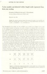
Constraints on <strong>SUSY</strong> Models<br />
mSUGRA well-studied in literature: eg Ellis, Olive et al PLB565<br />
(2003) 176; Roszkowski et al JHEP 0108 (2001) 024; Baltz, Gondolo, JHEP 0410 (2004) 052;. . .<br />
800<br />
tan β = 10 , µ > 0<br />
700<br />
m h = 114 GeV<br />
m 0 (GeV)<br />
600<br />
500<br />
400<br />
m χ ± = 104 GeV<br />
300<br />
200<br />
100<br />
0<br />
100 200 300 400 500 600 700 800 900 1000<br />
m 1/2 (GeV)<br />
<strong>SUSY</strong> <strong>Dark</strong> <strong>Matter</strong> <strong>and</strong> <strong>Colliders</strong><br />
B.C. Allanach – p.11/53
Shortcomings<br />
• Really, would like to combine likelihoods from<br />
different measurements<br />
• Typically only 2d scans, but in general we have<br />
α s (M Z ), m t , m b , m 0 , M 1/2 , A 0 , tan β to vary<br />
• Effective 3d type scan done which<br />
parameterises a 2d surface of correct Ωh 2<br />
• Baltz et al managed to perform a 4d scan, but lost<br />
the likelihood interpretation. They used the<br />
impressive Markov Chain Monte Carlo<br />
technique.<br />
Done in 2d in Ellis et al, hep-ph/0310356<br />
Ellis et al, hep-ph/0411218<br />
<strong>SUSY</strong> <strong>Dark</strong> <strong>Matter</strong> <strong>and</strong> <strong>Colliders</strong><br />
B.C. Allanach – p.12/53
Markov-Chain Monte Carlo<br />
Markov chain consists of list of parameter points x ( t)<br />
<strong>and</strong> associated likelihoods L (t)<br />
1. Pick a point at r<strong>and</strong>om for x (1)<br />
2. Pick a point around x (t) (say with a Gaussian<br />
width) as the potential new point.<br />
3. If L (t+1) > L (t) , the new point is appended onto<br />
the chain. Otherwise, the proposed point is<br />
accepted with probability L (t+1) /L (t) . If not<br />
accepted, a copy of x (t) is added on to the chain.<br />
Final density of x points ∝ L. Required number of<br />
points goes linearly with number of dimensions.<br />
<strong>SUSY</strong> <strong>Dark</strong> <strong>Matter</strong> <strong>and</strong> <strong>Colliders</strong><br />
B.C. Allanach – p.13/53
Implementation<br />
Input parameters are: m 0 , A 0 , M 1/2 , tan β<br />
• m t = 172.7 ± 2.9 GeV<br />
• m b (m b ) MS = 4.2 ± 0.2 GeV,<br />
• α s (M Z ) MS = 0.1187 ± 0.002.<br />
For the likelihood, we also use<br />
• Ω DM h 2 = 0.1125 +0.0081<br />
−0.0091<br />
• δ(g − 2) µ /2 = (19 ± 8.4) × 10 −10<br />
• BR[b → sγ] = (3.52 ± 0.42) × 10 −5<br />
<strong>SUSY</strong> <strong>Dark</strong> <strong>Matter</strong> <strong>and</strong> <strong>Colliders</strong><br />
ln L = − 1 2<br />
∑<br />
i<br />
(p i − m i ) 2<br />
2σ 2 i<br />
+ c<br />
B.C. Allanach – p.14/53
Convergence<br />
We run 9×1 000 000 points. By comparing the 9<br />
independent chains with r<strong>and</strong>om starting points, we<br />
can provide a statistical measure of convergence: an<br />
upper bound r on the excepted variance decrease for<br />
infinite statistics.<br />
2<br />
upper bound<br />
1.8<br />
1.6<br />
r<br />
1.4<br />
1.2<br />
<strong>SUSY</strong> <strong>Dark</strong> <strong>Matter</strong> <strong>and</strong> <strong>Colliders</strong><br />
1<br />
10 20 30 40 50 60 70 80 90 100<br />
step/10000<br />
B.C. Allanach – p.15/53
m 0 (TeV)<br />
2<br />
1.8<br />
1.6<br />
1.4<br />
1.2<br />
1<br />
0.8<br />
0.6<br />
0.4<br />
0.2<br />
0<br />
L/L(max)<br />
0 0.5 1 1.5 2<br />
M 1/2 (TeV)<br />
1<br />
0.9<br />
0.8<br />
0.7<br />
0.6<br />
0.5<br />
0.4<br />
0.3<br />
0.2<br />
0.1<br />
0<br />
m 0 (TeV)<br />
2<br />
1.8<br />
1.6<br />
1.4<br />
1.2<br />
1<br />
0.8<br />
0.6<br />
0.4<br />
0.2<br />
0<br />
L/L(max)<br />
0 10 20 30 40 50 60<br />
tan β<br />
1<br />
0.9<br />
0.8<br />
0.7<br />
0.6<br />
0.5<br />
0.4<br />
0.3<br />
0.2<br />
0.1<br />
0<br />
m 1/2 (TeV)<br />
2<br />
1.8<br />
1.6<br />
1.4<br />
1.2<br />
1<br />
0.8<br />
0.6<br />
0.4<br />
0.2<br />
0<br />
L/L(max)<br />
0 10 20 30 40 50 60<br />
1<br />
0.9<br />
0.8<br />
0.7<br />
0.6<br />
0.5<br />
0.4<br />
0.3<br />
0.2<br />
0.1<br />
0<br />
A 0 (TeV)<br />
2<br />
1.5<br />
1<br />
0.5<br />
0<br />
-0.5<br />
-1<br />
-1.5<br />
-2<br />
L/L(max)<br />
0 10 20 30 40 50 60<br />
1<br />
0.9<br />
0.8<br />
0.7<br />
0.6<br />
0.5<br />
0.4<br />
0.3<br />
0.2<br />
0.1<br />
0<br />
tan β<br />
tan β<br />
<strong>SUSY</strong> <strong>Dark</strong> <strong>Matter</strong> <strong>and</strong> <strong>Colliders</strong><br />
B.C. Allanach – p.16/53
Annihilation Mechanism<br />
Define stau co-annihilation when m˜τ is within 10% of<br />
m χ<br />
0<br />
1<br />
<strong>and</strong> Higgs pole when m h,A is within 10% of<br />
2m χ<br />
0<br />
1<br />
.<br />
Region likelihood<br />
h 0 pole 0.02±0.01<br />
A 0 pole 0.41±0.03<br />
˜τ co-an 0.27±0.04<br />
˜t co-an (2.1 ± 4.8) × 10 −4<br />
Table 0: Likelihood of being in a certain region of<br />
mSUGRA parameter space.<br />
Likelihood of chain ˜q L → χ 0 2 → ˜l R → χ 0 1 is 24±4%<br />
<strong>SUSY</strong> <strong>Dark</strong> <strong>Matter</strong> <strong>and</strong> <strong>Colliders</strong><br />
B.C. Allanach – p.17/53
m χ1<br />
0 (TeV)<br />
0.9<br />
0.8<br />
0.7<br />
0.6<br />
0.5<br />
0.4<br />
0.3<br />
0.2<br />
0.1<br />
0<br />
80 90 100 110 120 130 140<br />
m h (GeV)<br />
L/L(max)<br />
1<br />
0.9<br />
0.8<br />
0.7<br />
0.6<br />
0.5<br />
0.4<br />
0.3<br />
0.2<br />
0.1<br />
0<br />
m χ1<br />
0 (TeV)<br />
0.9<br />
0.8<br />
0.7<br />
0.6<br />
0.5<br />
0.4<br />
0.3<br />
0.2<br />
0.1<br />
0<br />
0 0.5 1 1.5 2 2.5<br />
m A (TeV)<br />
L/L(max)<br />
1<br />
0.9<br />
0.8<br />
0.7<br />
0.6<br />
0.5<br />
0.4<br />
0.3<br />
0.2<br />
0.1<br />
0<br />
m χ1<br />
0 (TeV)<br />
0.9<br />
0.8<br />
0.7<br />
0.6<br />
0.5<br />
0.4<br />
0.3<br />
0.2<br />
0.1<br />
0<br />
0 0.5 1 1.5 2<br />
m τ (TeV)<br />
L/L(max)<br />
1<br />
0.9<br />
0.8<br />
0.7<br />
0.6<br />
0.5<br />
0.4<br />
0.3<br />
0.2<br />
0.1<br />
0<br />
L per bin<br />
0.06<br />
0.05<br />
0.04<br />
0.03<br />
0.02<br />
0.01<br />
0<br />
RH slepton<br />
gluino<br />
LH squark<br />
light stop<br />
0 0.5 1 1.5 2 2.5 3 3.5 4<br />
m (TeV)<br />
<strong>SUSY</strong> <strong>Dark</strong> <strong>Matter</strong> <strong>and</strong> <strong>Colliders</strong><br />
B.C. Allanach – p.18/53
0.0015<br />
0.03<br />
0.08<br />
L/GeV<br />
0.001<br />
0.0005<br />
0.02<br />
0.01<br />
0<br />
20%<br />
0 10 20 30<br />
L/bin<br />
0.07<br />
0.06<br />
0.05<br />
0.04<br />
0.03<br />
0.02<br />
0.01<br />
29%<br />
tanβ<br />
60<br />
50<br />
40<br />
30<br />
20<br />
10<br />
0<br />
0<br />
37<br />
400<br />
800 1200<br />
m τ - m 0 χ1<br />
(GeV)<br />
0 0.5 1 1.5 2<br />
m A (TeV)<br />
1600<br />
L/L(max)<br />
2000<br />
1<br />
0.9<br />
0.8<br />
0.7<br />
0.6<br />
0.5<br />
0.4<br />
0.3<br />
0.2<br />
0.1<br />
0<br />
log 10 [BR(B s -> µµ)]<br />
-4<br />
-5<br />
-6<br />
-7<br />
-8<br />
-9<br />
0<br />
-9 -8.5 -8 -7.5 -7 -6.5 -6<br />
log 10 (BR[B s ->µµ])<br />
-10.5 -10 -9.5 -9 -8.5<br />
log 10 [δ(g-2) µ /2]<br />
L/L(max)<br />
1<br />
0.9<br />
0.8<br />
0.7<br />
0.6<br />
0.5<br />
0.4<br />
0.3<br />
0.2<br />
0.1<br />
0<br />
<strong>SUSY</strong> <strong>Dark</strong> <strong>Matter</strong> <strong>and</strong> <strong>Colliders</strong><br />
B.C. Allanach – p.19/53
Caveats<br />
• Implicitly assumed that LSP constitutes all of<br />
dark matter<br />
• Assumed radiation domination in post-inflation<br />
era. No clear evidence between freeze-out+BBN<br />
that this is the case (t eq changes).<br />
• Examples of non-st<strong>and</strong>ard cosmology that would<br />
change the prediction:<br />
• Extra degrees of freedom<br />
• Low reheating temperature<br />
• Extra dimensional models<br />
• Anisotropic cosmologies<br />
• Non-thermal production of neutralinos (late<br />
decays)<br />
<strong>SUSY</strong> <strong>Dark</strong> <strong>Matter</strong> <strong>and</strong> <strong>Colliders</strong><br />
B.C. Allanach – p.20/53
LHC (ATLAS)<br />
<strong>SUSY</strong> <strong>Dark</strong> <strong>Matter</strong> <strong>and</strong> <strong>Colliders</strong><br />
B.C. Allanach – p.21/53
Collider <strong>SUSY</strong> <strong>Dark</strong> <strong>Matter</strong><br />
Production<br />
Strong sparticle production <strong>and</strong> decay to dark matter<br />
particles.<br />
7 TeV<br />
p<br />
q<br />
q<br />
q<br />
q<br />
p<br />
7 TeV<br />
q,g<br />
q,g<br />
q<br />
Interaction<br />
q<br />
~ q<br />
~<br />
q<br />
χ 0 1<br />
χ 0 1<br />
Q: Can we measure enough to predict σ<br />
<strong>SUSY</strong> <strong>Dark</strong> <strong>Matter</strong> <strong>and</strong> <strong>Colliders</strong><br />
B.C. Allanach – p.22/53
Collider <strong>SUSY</strong> <strong>Dark</strong> <strong>Matter</strong><br />
Production<br />
Strong sparticle production <strong>and</strong> decay to dark matter<br />
particles.<br />
7 TeV<br />
p<br />
q<br />
q<br />
q<br />
q<br />
p<br />
7 TeV<br />
q,g<br />
q,g<br />
q<br />
Interaction<br />
q<br />
~ q<br />
~<br />
q<br />
χ 0 1<br />
Any dark matter c<strong>and</strong>idate that couples to hadrons can<br />
be produced at the LHC<br />
χ 0 1<br />
<strong>SUSY</strong> <strong>Dark</strong> <strong>Matter</strong> <strong>and</strong> <strong>Colliders</strong><br />
B.C. Allanach – p.22/53
LHC vs LC in <strong>SUSY</strong><br />
Measurement<br />
• LHC (start date 2007) produces strongly<br />
interacting particles up to a few TeV. Precision<br />
measurements of mass differences possible if the<br />
decay chains exist: possibly per mille for leptons,<br />
several percent for jets.<br />
• ILC has several energy options: 500-1000 GeV,<br />
CLIC up to 3 TeV. Linear colliders produce less<br />
strong particles but much easier to make<br />
precision measurements of masses/couplings.<br />
Q: What energy for LC<br />
Q: What do we get from LHC <br />
LHC/ILC Working Group Report: hep-ph/0410364<br />
<strong>SUSY</strong> <strong>Dark</strong> <strong>Matter</strong> <strong>and</strong> <strong>Colliders</strong><br />
B.C. Allanach – p.23/53
Coannihilation Slope<br />
annihilation (%)<br />
70<br />
60<br />
50<br />
40<br />
30<br />
20<br />
0 0<br />
χ 1 χ1<br />
0 ~<br />
χ 1 τ<br />
~ ~<br />
τ τ<br />
0 ~<br />
χ 1 l<br />
~ ~<br />
l~ (τ /l )<br />
~ ~<br />
l =µ or<br />
~<br />
e<br />
10<br />
0<br />
100 150 200 250 300 350 400<br />
m~ (GeV)<br />
τ<br />
m 2˜lR ≈ m 2 0 + 0.15M 2 1/2 , M χ 0 1 ≈ 0.4M 1/2<br />
Low enough M 1/2 ⇒ quasi-deegenerate ˜τ, M χ<br />
0<br />
1<br />
<strong>SUSY</strong> <strong>Dark</strong> <strong>Matter</strong> <strong>and</strong> <strong>Colliders</strong><br />
B.C. Allanach – p.24/53
Coannihilation Slope<br />
annihilation (%)<br />
70<br />
60<br />
50<br />
40<br />
30<br />
20<br />
0 0<br />
χ 1 χ1<br />
0 ~<br />
χ 1 τ<br />
~ ~<br />
τ τ<br />
0 ~<br />
χ 1 l<br />
~ ~<br />
l~ (τ /l )<br />
~ ~<br />
l =µ or<br />
~<br />
e<br />
10<br />
0<br />
100 150 200 250 300 350 400<br />
m~ (GeV)<br />
τ<br />
m 2˜lR ≈ m 2 0 + 0.15M 2 1/2 , M χ 0 1 ≈ 0.4M 1/2<br />
If we do not assume mSUGRA, we will also have to<br />
measure selectron <strong>and</strong> smuon properties.<br />
<strong>SUSY</strong> <strong>Dark</strong> <strong>Matter</strong> <strong>and</strong> <strong>Colliders</strong><br />
B.C. Allanach – p.24/53
Coannihilation Theory<br />
Uncertainties<br />
Ωh 2<br />
0.145<br />
0.14<br />
0.135<br />
0.13<br />
0.125<br />
0.12<br />
0.115<br />
Ωh 2<br />
Scale variation<br />
Ωh 2<br />
0.18<br />
0.16<br />
0.14<br />
0.12<br />
0.1<br />
0.08<br />
0.06<br />
0.04<br />
-1 loop tau Yukawa<br />
full calculation<br />
-1 loop neutralino<br />
-2 loop gaugino RGEs<br />
0.11<br />
100 150 200 250 300 350 400<br />
M~ (GeV)<br />
τ<br />
0.02<br />
100 150 200 250 300 350 400 450<br />
M~ (GeV)<br />
τ<br />
Expect higher orders to be 100 times smaller than these<br />
differences: 3-loop terms could possibly be important!<br />
<strong>SUSY</strong> <strong>Dark</strong> <strong>Matter</strong> <strong>and</strong> <strong>Colliders</strong><br />
B.C. Allanach – p.25/53
Coannihilation Theory<br />
Uncertainties<br />
Ωh 2<br />
0.145<br />
0.14<br />
0.135<br />
0.13<br />
0.125<br />
0.12<br />
0.115<br />
Ωh 2<br />
Scale variation<br />
Ωh 2<br />
0.18<br />
0.16<br />
0.14<br />
0.12<br />
0.1<br />
0.08<br />
0.06<br />
0.04<br />
-1 loop tau Yukawa<br />
full calculation<br />
-1 loop neutralino<br />
-2 loop gaugino RGEs<br />
0.11<br />
100 150 200 250 300 350 400<br />
M~ (GeV)<br />
τ<br />
0.02<br />
100 150 200 250 300 350 400 450<br />
M~ (GeV)<br />
τ<br />
Effect of 2-loop RGE terms suggest a possible effect<br />
from 3 loops. Jack <strong>and</strong> Jones find that it’s not significant<br />
for the neutralino.<br />
<strong>SUSY</strong> <strong>Dark</strong> <strong>Matter</strong> <strong>and</strong> <strong>Colliders</strong><br />
B.C. Allanach – p.25/53
Iterative Procedure<br />
What change in a parameter produces a 10% change<br />
in Ωh 2 <br />
Take a parameter point with ω −1 ≡ Ωh 2 . Change one<br />
parameter at a time by fraction a 0 . Result is ω 0 , then<br />
iterate<br />
a i+1 = a i ω −1<br />
10%<br />
w i − ω −1<br />
.<br />
Small accuracy a ≡ a ∞ means the parameter has to<br />
be known very accurately in order to predict Ωh 2 to<br />
10%.<br />
For parameters that are zero, we take the absolute value<br />
as a rather than the fractional value.<br />
<strong>SUSY</strong> <strong>Dark</strong> <strong>Matter</strong> <strong>and</strong> <strong>Colliders</strong><br />
B.C. Allanach – p.26/53
Uncertainties<br />
We use two approaches to determine what variation of<br />
parameters produce a 10% variation in Ωh 2 :<br />
• PmSUGRA - variation of weak scale parameters<br />
(not on mSUGRA trajectory): m χ<br />
0<br />
1<br />
, M A , m b etc.<br />
• mSUGRA - simple variation of mSUGRA<br />
parameters <strong>and</strong> experimental inputs:<br />
m 0 , M 1/2 , α s (M Z ), m t etc.<br />
mSUGRA theory uncertainties estimated by varying<br />
scale at which radiative corrections added to sparticle<br />
masses:<br />
0.5 < x ≡ M <strong>SUSY</strong><br />
√ m˜t 1<br />
m˜t 2<br />
< 2, M <strong>SUSY</strong> > M Z<br />
<strong>SUSY</strong> <strong>Dark</strong> <strong>Matter</strong> <strong>and</strong> <strong>Colliders</strong><br />
B.C. Allanach – p.27/53
mSUGRA Coannihilation<br />
Uncertainties<br />
a<br />
0.16<br />
0.14<br />
0.12<br />
0.1<br />
0.08<br />
0.06<br />
0.04<br />
0.02<br />
a(M 1/2 )<br />
a(m 0 )<br />
∆A 0<br />
-<br />
a(tanβ)<br />
180<br />
160<br />
140<br />
120<br />
100<br />
80<br />
0<br />
60<br />
100 150 200 250 300 350 400 450<br />
m~ (GeV)<br />
τ<br />
∆A 0<br />
- (GeV)<br />
a(m 0 ) ≈ a(M 1/2 ) comes from the sensitivity to<br />
exp[−(m˜τ − M χ<br />
0<br />
1<br />
)]<br />
<strong>SUSY</strong> <strong>Dark</strong> <strong>Matter</strong> <strong>and</strong> <strong>Colliders</strong><br />
B.C. Allanach – p.28/53
mSUGRA Coannihilation<br />
Uncertainties<br />
a<br />
0.16<br />
0.14<br />
0.12<br />
0.1<br />
0.08<br />
0.06<br />
0.04<br />
0.02<br />
a(M 1/2 )<br />
a(m 0 )<br />
∆A 0<br />
-<br />
a(tanβ)<br />
180<br />
160<br />
140<br />
120<br />
100<br />
80<br />
0<br />
60<br />
100 150 200 250 300 350 400 450<br />
m~ (GeV)<br />
τ<br />
∆A 0<br />
- (GeV)<br />
Unknown whether accuracies can be reached - but it<br />
looks difficult<br />
region.<br />
Polesello, Tovey, JHEP05 (2004) 071<br />
<strong>SUSY</strong> <strong>Dark</strong> <strong>Matter</strong> <strong>and</strong> <strong>Colliders</strong><br />
: ∆Ωh 2 ∼ .03 in diminished bulk<br />
B.C. Allanach – p.28/53
PmSUGRA Coannihilation<br />
a(tanβ, µ)<br />
0.6<br />
0.007<br />
1400<br />
tanβ<br />
χ 0 2<br />
µ<br />
0.5<br />
M 1<br />
1200<br />
χ 0 3<br />
0.006<br />
χ 0 4<br />
1000<br />
~<br />
0.4<br />
eR<br />
0.005<br />
~<br />
e<br />
800<br />
L<br />
~<br />
0.3<br />
τ 2<br />
0.004<br />
600<br />
0.2<br />
400<br />
0.003<br />
0.1<br />
200<br />
0.002<br />
100 150 200 250 300 350 400<br />
100 150 200 250 300 350 400 450<br />
m~ (GeV) M<br />
τ χ<br />
0 (GeV)<br />
1<br />
a(M 1 )<br />
mass (GeV)<br />
RHS: Spectrum useful for optimal energy of linear collider.<br />
ẽ R , ˜µ R also possible. Cascade ˜q L → χ 0 2 → ẽ R →<br />
χ 0 1 available.<br />
<strong>SUSY</strong> <strong>Dark</strong> <strong>Matter</strong> <strong>and</strong> <strong>Colliders</strong><br />
B.C. Allanach – p.29/53
PmSUGRA Coannihilation<br />
a(tanβ, µ)<br />
0.6<br />
0.007<br />
1400<br />
tanβ<br />
χ 0 2<br />
µ<br />
0.5<br />
M 1<br />
1200<br />
χ 0 3<br />
0.006<br />
χ 0 4<br />
1000<br />
~<br />
0.4<br />
eR<br />
0.005<br />
~<br />
e<br />
800<br />
L<br />
~<br />
0.3<br />
τ 2<br />
0.004<br />
600<br />
0.2<br />
400<br />
0.003<br />
0.1<br />
200<br />
0.002<br />
100 150 200 250 300 350 400<br />
100 150 200 250 300 350 400 450<br />
m~ (GeV) M<br />
τ χ<br />
0 (GeV)<br />
1<br />
a(M 1 )<br />
LHS: Dependences in left-h<strong>and</strong> plot all come from the<br />
effect on LSP mass.<br />
Need to know M χ<br />
0<br />
1<br />
very accurately.<br />
mass (GeV)<br />
<strong>SUSY</strong> <strong>Dark</strong> <strong>Matter</strong> <strong>and</strong> <strong>Colliders</strong><br />
B.C. Allanach – p.29/53
PmSUGRA Dependencies<br />
∆M (GeV)<br />
10<br />
1<br />
0.4<br />
∆M<br />
9<br />
cos2θ τ 0.99 0.35<br />
8<br />
0.98<br />
7<br />
0.3<br />
6<br />
0.97<br />
0.25<br />
5<br />
0.96<br />
4<br />
0.2<br />
0.95<br />
3<br />
0.15<br />
0.94<br />
2<br />
1<br />
0.93<br />
0.1<br />
0<br />
0.92 0.05<br />
100 150 200 250 300 350 400 450<br />
m~ (GeV) τ<br />
cos2θ τ<br />
-<br />
∆cos2θ τ required, a(M)<br />
∆cos2θ τ<br />
- required<br />
δM required<br />
a(M χ )<br />
1.3<br />
1.2<br />
1.1<br />
0.9<br />
0.8<br />
0.7<br />
0.6<br />
100 150 200 250 300 350 400 450<br />
m~<br />
τ (GeV)<br />
1<br />
δM required (GeV)<br />
LHS: plots of quantities along mSUGRA slope. Below<br />
∆M = 1.78 GeV, no two-body stau decay. LC studies<br />
indicate ∆M > 5 GeV is OK.<br />
<strong>SUSY</strong> <strong>Dark</strong> <strong>Matter</strong> <strong>and</strong> <strong>Colliders</strong><br />
B.C. Allanach – p.30/53
PmSUGRA Dependencies<br />
∆M (GeV)<br />
10<br />
1<br />
0.4<br />
∆M<br />
9<br />
cos2θ τ 0.99 0.35<br />
8<br />
0.98<br />
7<br />
0.3<br />
6<br />
0.97<br />
0.25<br />
5<br />
0.96<br />
4<br />
0.2<br />
0.95<br />
3<br />
0.15<br />
0.94<br />
2<br />
1<br />
0.93<br />
0.1<br />
0<br />
0.92 0.05<br />
100 150 200 250 300 350 400 450<br />
m~ (GeV) τ<br />
cos2θ τ<br />
-<br />
∆cos2θ τ required, a(M)<br />
∆cos2θ τ<br />
- required<br />
δM required<br />
a(M χ )<br />
1.3<br />
1.2<br />
1.1<br />
0.9<br />
0.8<br />
0.7<br />
0.6<br />
100 150 200 250 300 350 400 450<br />
m~<br />
τ (GeV)<br />
1<br />
δM required (GeV)<br />
˜τ 1 χ 0 1 → τγ ∝ 3 cos 2θ τ + 5 from coupling of neutralino<br />
to ˜τ L/R .<br />
<strong>SUSY</strong> <strong>Dark</strong> <strong>Matter</strong> <strong>and</strong> <strong>Colliders</strong><br />
B.C. Allanach – p.30/53
PmSUGRA Dependencies<br />
∆M (GeV)<br />
10<br />
1<br />
0.4<br />
∆M<br />
9<br />
cos2θ τ 0.99 0.35<br />
8<br />
0.98<br />
7<br />
0.3<br />
6<br />
0.97<br />
0.25<br />
5<br />
0.96<br />
4<br />
0.2<br />
0.95<br />
3<br />
0.15<br />
0.94<br />
2<br />
1<br />
0.93<br />
0.1<br />
0<br />
0.92 0.05<br />
100 150 200 250 300 350 400 450<br />
m~ (GeV) τ<br />
cos2θ τ<br />
-<br />
∆cos2θ τ required, a(M)<br />
∆cos2θ τ<br />
- required<br />
δM required<br />
a(M χ )<br />
1.3<br />
1.2<br />
1.1<br />
0.9<br />
0.8<br />
0.7<br />
0.6<br />
100 150 200 250 300 350 400 450<br />
m~<br />
τ (GeV)<br />
1<br />
δM required (GeV)<br />
a(M χ ) found by keeping ∆M constant, δM by just<br />
varying stau mass. mẽ, m˜µ needed to about 1.5%<br />
<strong>SUSY</strong> <strong>Dark</strong> <strong>Matter</strong> <strong>and</strong> <strong>Colliders</strong><br />
B.C. Allanach – p.30/53
Slepton Dependence<br />
7<br />
δ - (∆M)<br />
6<br />
GeV<br />
5<br />
4<br />
3<br />
2<br />
150 200 250 300 350 400 450<br />
m~ (GeV)<br />
e<br />
Accuracy required on m˜l<br />
− m χ<br />
0<br />
1<br />
for WMAP precision.<br />
LC studies say this is acheivable, but need more work<br />
for cos θ τ (=0.987±0.06 at lower end of slope).<br />
<strong>SUSY</strong> <strong>Dark</strong> <strong>Matter</strong> <strong>and</strong> <strong>Colliders</strong><br />
B.C. Allanach – p.31/53
Summary<br />
• Markov chains bring out the multi-dimensionality<br />
of the space: is a lot less constrained than in 2d<br />
• Still, current data is constraining<br />
• LHC could produce copious amounts of <strong>SUSY</strong><br />
dark matter<br />
• Want to measure σ in order to predict Ωh 2 <strong>and</strong><br />
test cosmological assumptions<br />
• 10% accuracy will require ILC+LHC data<br />
• Can control many uncertainties by measuring<br />
additional quantities: Γ A , m˜τ − M χ<br />
0<br />
1<br />
, . . .<br />
• Non mSUGRA case could well be easier.<br />
• Have not discussed direct detection yet<br />
<strong>SUSY</strong> <strong>Dark</strong> <strong>Matter</strong> <strong>and</strong> <strong>Colliders</strong><br />
B.C. Allanach – p.32/53
Supplementary Material<br />
<strong>SUSY</strong> <strong>Dark</strong> <strong>Matter</strong> <strong>and</strong> <strong>Colliders</strong><br />
B.C. Allanach – p.33/53
Likelihood<br />
L ≡ p(d|m) is pdf of reproducing data d assuming<br />
mSUGRA model m (which depends on parameters).<br />
p(m|d) = p(d|m) p(m)<br />
p(d)<br />
p(m 1 |d)<br />
p(m 2 |d)<br />
= p(d|m 1)p(m 1 )<br />
p(d|m 2 )p(m 2 )<br />
Thus, you can interpret the likelihood distribution as<br />
relative probabilities if your ratio of priors is 1. Otherwise,<br />
convolute it with YOUR priors!<br />
<strong>SUSY</strong> <strong>Dark</strong> <strong>Matter</strong> <strong>and</strong> <strong>Colliders</strong><br />
B.C. Allanach – p.34/53
Funnel Slope<br />
GeV<br />
1400<br />
1200<br />
1000<br />
800<br />
600<br />
m(χ 1 )<br />
m(χ 3 )<br />
Γ A<br />
µ<br />
m(l R )<br />
m(l L )<br />
m(χ 2 )<br />
35<br />
30<br />
25<br />
20<br />
Γ A (GeV)<br />
~<br />
400<br />
200<br />
15<br />
0<br />
300 400 500 600 700 800 900 1000 10<br />
M A (GeV)<br />
< σv > −1 ∼ 4m χ 0Γ ( ( ) )<br />
A MA − 2m 2<br />
1 χ<br />
0<br />
g 2 4 1<br />
+ 1<br />
m χ 0 ˜χ 0 1 A Γ A<br />
1<br />
.<br />
<strong>SUSY</strong> <strong>Dark</strong> <strong>Matter</strong> <strong>and</strong> <strong>Colliders</strong><br />
B.C. Allanach – p.35/53
Funnel Slope<br />
GeV<br />
1400<br />
1200<br />
1000<br />
800<br />
600<br />
m(χ 1 )<br />
m(χ 3 )<br />
Γ A<br />
µ<br />
m(l R )<br />
m(l L )<br />
m(χ 2 )<br />
35<br />
30<br />
25<br />
20<br />
Γ A (GeV)<br />
~<br />
400<br />
200<br />
15<br />
0<br />
300 400 500 600 700 800 900 1000 10<br />
M A (GeV)<br />
Notice that spectrum is quite heavy: need a high energy<br />
ILC! Γ A will be important.<br />
<strong>SUSY</strong> <strong>Dark</strong> <strong>Matter</strong> <strong>and</strong> <strong>Colliders</strong><br />
B.C. Allanach – p.35/53
Funnel Theory Uncertainties<br />
Ωh 2<br />
0.5<br />
0.45<br />
0.4<br />
0.35<br />
0.3<br />
0.25<br />
0.2<br />
0.15<br />
0.1<br />
0.05<br />
full calculation<br />
no m b resummation<br />
1 loop Higgs RGEs<br />
1 loop gaugino RGEs<br />
-2 loop QCD mt correction<br />
Ωh 2<br />
0.145<br />
0.14<br />
0.135<br />
0.13<br />
0.125<br />
0.12<br />
0.115<br />
Ωh 2<br />
(M A - 2M χ1<br />
0)/Γ A<br />
1.65<br />
1.6<br />
1.55<br />
1.5<br />
1.45<br />
1.4<br />
(M A - 2M χ1<br />
0)/Γ A<br />
0<br />
300 400 500 600 700 800 900 10001100<br />
M A (GeV)<br />
0.11<br />
0.6 0.8 1 1.2 1.4<br />
x<br />
1.35<br />
LHS: Γ A affected by large m SM<br />
b<br />
/(1 + ∆ <strong>SUSY</strong> ) corrections<br />
since A → b¯b ∝ Ab¯b coupling ∝ m b tan β, <strong>and</strong><br />
tan β = 50.<br />
<strong>SUSY</strong> <strong>Dark</strong> <strong>Matter</strong> <strong>and</strong> <strong>Colliders</strong><br />
B.C. Allanach – p.36/53
Funnel Theory Uncertainties<br />
Ωh 2<br />
0.5<br />
0.45<br />
0.4<br />
0.35<br />
0.3<br />
0.25<br />
0.2<br />
0.15<br />
0.1<br />
0.05<br />
full calculation<br />
no m b resummation<br />
1 loop Higgs RGEs<br />
1 loop gaugino RGEs<br />
-2 loop QCD mt correction<br />
Ωh 2<br />
0.145<br />
0.14<br />
0.135<br />
0.13<br />
0.125<br />
0.12<br />
0.115<br />
Ωh 2<br />
(M A - 2M χ1<br />
0)/Γ A<br />
1.65<br />
1.6<br />
1.55<br />
1.5<br />
1.45<br />
1.4<br />
(M A - 2M χ1<br />
0)/Γ A<br />
0<br />
300 400 500 600 700 800 900 10001100<br />
M A (GeV)<br />
0.11<br />
0.6 0.8 1 1.2 1.4<br />
x<br />
1.35<br />
RHS: x > 1.5 yielded MA 2 < 0 ie no EWSB. Strong<br />
correlation of theory error with its effect on (M A −<br />
2M χ<br />
0<br />
1<br />
)/Γ A - could measure it!<br />
<strong>SUSY</strong> <strong>Dark</strong> <strong>Matter</strong> <strong>and</strong> <strong>Colliders</strong><br />
B.C. Allanach – p.36/53
Funnel Accuracies<br />
LHS: mSUGRA. a(m b ) worrying. α s (M Z )<br />
dependence comes about through its effect on<br />
m b (m b ). m 0 , M 1/2 might be feasible at LHC, m t<br />
possible at ILC. tan β looks impossible.<br />
a<br />
10<br />
1<br />
0.1<br />
0.01<br />
0.001<br />
M 1/2<br />
-<br />
m t<br />
α s (M Z )<br />
m b<br />
m 0<br />
∆A 0<br />
tanβ<br />
0<br />
50 100 150 200 250 300 350 400 450 500<br />
m 0 χ1<br />
(GeV)<br />
200<br />
150<br />
100<br />
50<br />
∆A 0 (GeV)<br />
a<br />
100<br />
10<br />
1<br />
0.1<br />
0.01<br />
a(Γ A )<br />
a(M χ1<br />
0)<br />
a(M A )<br />
a(2M χ1<br />
0 - M A )<br />
a(µ)<br />
2M χ1<br />
0 - M A<br />
-20<br />
-40<br />
-60<br />
-80<br />
-100<br />
-120<br />
50 100 150 200 250 300 350 400 450 500<br />
M 0 χ1<br />
(GeV)<br />
0<br />
2M χ1<br />
0 - M A (GeV)<br />
<strong>SUSY</strong> <strong>Dark</strong> <strong>Matter</strong> <strong>and</strong> <strong>Colliders</strong><br />
B.C. Allanach – p.37/53
Funnel Accuracies<br />
SM inputs <strong>and</strong> tan β uncertainties can be controlled<br />
by measuring M A , Γ A . Aχ 0 1χ 0 1 coupling ∼ 1/µ.<br />
Γ A ∝ M A tan 2 β(m 2 b + m2 τ) (γγ option of LC,<br />
A → µµ at LHC).<br />
a<br />
10<br />
1<br />
0.1<br />
0.01<br />
0.001<br />
M 1/2<br />
-<br />
m t<br />
α s (M Z )<br />
m b<br />
m 0<br />
∆A 0<br />
tanβ<br />
0<br />
50 100 150 200 250 300 350 400 450 500<br />
m 0 χ1<br />
(GeV)<br />
200<br />
150<br />
100<br />
50<br />
∆A 0 (GeV)<br />
a<br />
100<br />
10<br />
1<br />
0.1<br />
0.01<br />
a(Γ A )<br />
a(M χ1<br />
0)<br />
a(M A )<br />
a(2M χ1<br />
0 - M A )<br />
a(µ)<br />
2M χ1<br />
0 - M A<br />
-20<br />
-40<br />
-60<br />
-80<br />
-100<br />
-120<br />
50 100 150 200 250 300 350 400 450 500<br />
M 0 χ1<br />
(GeV)<br />
0<br />
2M χ1<br />
0 - M A (GeV)<br />
<strong>SUSY</strong> <strong>Dark</strong> <strong>Matter</strong> <strong>and</strong> <strong>Colliders</strong><br />
B.C. Allanach – p.37/53
Funnel Accuracies<br />
Mass of χ 0 1 is important, but not mixing (see a(µ)).<br />
a<br />
10<br />
1<br />
0.1<br />
0.01<br />
0.001<br />
M 1/2<br />
-<br />
m t<br />
α s (M Z )<br />
m b<br />
m 0<br />
∆A 0<br />
tanβ<br />
0<br />
50 100 150 200 250 300 350 400 450 500<br />
m 0 χ1<br />
(GeV)<br />
200<br />
150<br />
100<br />
50<br />
∆A 0 (GeV)<br />
a<br />
100<br />
10<br />
1<br />
0.1<br />
0.01<br />
a(Γ A )<br />
a(M χ1<br />
0)<br />
a(M A )<br />
a(2M χ1<br />
0 - M A )<br />
a(µ)<br />
2M χ1<br />
0 - M A<br />
-20<br />
-40<br />
-60<br />
-80<br />
-100<br />
-120<br />
50 100 150 200 250 300 350 400 450 500<br />
M 0 χ1<br />
(GeV)<br />
0<br />
2M χ1<br />
0 - M A (GeV)<br />
<strong>SUSY</strong> <strong>Dark</strong> <strong>Matter</strong> <strong>and</strong> <strong>Colliders</strong><br />
B.C. Allanach – p.37/53
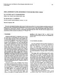
Focus Point Slope<br />
mass (GeV)<br />
1000<br />
900<br />
800<br />
700<br />
600<br />
500<br />
400<br />
300<br />
200<br />
M χ1<br />
0<br />
χ 2<br />
0<br />
χ 3<br />
0<br />
µ<br />
χ 4<br />
0<br />
M 1<br />
M 2<br />
100<br />
150 200 250 300 350 400 450<br />
M 0 χ1<br />
(GeV)<br />
Heavy sfermions <strong>and</strong> A 0 . M 1 < µ < M 2 , ie significant<br />
Higgsino component ∼ 25%.<br />
<strong>SUSY</strong> <strong>Dark</strong> <strong>Matter</strong> <strong>and</strong> <strong>Colliders</strong><br />
B.C. Allanach – p.38/53
Focus Channels <strong>and</strong> Theory<br />
annihilation (%)<br />
100<br />
80<br />
60<br />
40<br />
20<br />
coannihilation30<br />
annihilation<br />
tt -<br />
bb -<br />
WW/ZZ<br />
Zh,hh<br />
Ωh 2<br />
35<br />
25<br />
20<br />
15<br />
10<br />
-neutralinos<br />
-2 loop QCD<br />
-EW/Higgs<br />
-charginos<br />
non re-summed mb<br />
Full calculation<br />
-2 loop Higgs RGEs<br />
0<br />
150 200 250 300 350 400 450<br />
M χ<br />
0 (GeV)<br />
1<br />
5<br />
0<br />
1 2 3 4 5 6 7<br />
m 0 (TeV)<br />
t¯t annihilation predominantly through Z. Coannihilation<br />
≡ χ 0 1χ 0 i or χ0 1χ ± 1<br />
. Several competing channels.<br />
<strong>SUSY</strong> <strong>Dark</strong> <strong>Matter</strong> <strong>and</strong> <strong>Colliders</strong><br />
B.C. Allanach – p.39/53
Focus mSUGRA Accuracies<br />
a<br />
0.0003<br />
0.05<br />
45<br />
α s (M Z )<br />
∆A 0<br />
m t 0.045<br />
a(m 0 )<br />
a(M<br />
0.00025<br />
0.04<br />
1/2 )<br />
40<br />
a(tanβ)<br />
0.035<br />
35<br />
0.0002<br />
0.03<br />
0.06<br />
0.06<br />
0.05<br />
0.05 0.025<br />
30<br />
0.00015<br />
0.04<br />
0.04<br />
0.02<br />
0.03<br />
0.03<br />
25<br />
0.02<br />
0.02<br />
0.015<br />
0.0001<br />
0.01<br />
0.01 0.01<br />
m 20<br />
0<br />
b<br />
200 300 400 0 0.005<br />
5e-05<br />
0<br />
150 200 250 300 350 400 450 100 200 300 400 500 15<br />
M 0 χ1<br />
(GeV)<br />
M 0 χ1<br />
(GeV)<br />
a<br />
∆A 0 (GeV)<br />
∆A 0 (GeV)<br />
δm t = 30 MeV might be possible at future ILC but<br />
a(m 0 ) < 0.5% looks completely unfeasible.<br />
<strong>SUSY</strong> <strong>Dark</strong> <strong>Matter</strong> <strong>and</strong> <strong>Colliders</strong><br />
B.C. Allanach – p.40/53
Focus PmSUGRA Accuracies<br />
0.25<br />
0.2<br />
0.15<br />
m t<br />
M 2<br />
tanβ<br />
M 1<br />
µ<br />
M χ3<br />
0<br />
a<br />
0.1<br />
0.05<br />
0<br />
150 200 250 300 350 400 450<br />
M 0 χ1<br />
(GeV)<br />
Easier outside of mSUGRA, eg µ no longer sensitive<br />
to m t (∝ coupling to neutral goldstone).<br />
<strong>SUSY</strong> <strong>Dark</strong> <strong>Matter</strong> <strong>and</strong> <strong>Colliders</strong><br />
B.C. Allanach – p.41/53
LHC <strong>SUSY</strong> Measurements<br />
q l + l −<br />
˜q L χ 0 2 ˜l χ 0 1<br />
m 2 ll<br />
= (p l1 + p l2 ) 2 edge<br />
position measures<br />
√<br />
(m<br />
2<br />
χ 0 2−m 2˜l )(m 2˜l −m 2 χ 0 )<br />
1<br />
m 2˜l<br />
Events/0.5 GeV/100 fb -1<br />
400<br />
300<br />
200<br />
100<br />
205.7 / 197<br />
P1 2209.<br />
P2 108.7<br />
P3 1.291<br />
0<br />
0 50 100 150<br />
M ll<br />
(GeV)<br />
BCA, C Lester, A Parker, B Webber, JHEP 09 (2000) 004<br />
<strong>SUSY</strong> <strong>Dark</strong> <strong>Matter</strong> <strong>and</strong> <strong>Colliders</strong><br />
B.C. Allanach – p.42/53
Edge Fitting at S5 <strong>and</strong> O1<br />
200<br />
150<br />
100<br />
50<br />
400<br />
300<br />
200<br />
100<br />
200<br />
150<br />
100<br />
50<br />
300<br />
200<br />
100<br />
dσ/dmll (Events/100fb-1 /0.375GeV)<br />
dσ/dmllq (Events/100fb-1 /5GeV)<br />
0<br />
0<br />
0<br />
0<br />
0 50 100 150<br />
0 200 400 600 800 1000<br />
0 50 100 150<br />
0 200 400 600 800 1000<br />
(a) m ll (GeV)<br />
(b) m llq (GeV)<br />
(a) m ll (GeV)<br />
(b) m llq (GeV)<br />
400<br />
300<br />
200<br />
600<br />
400<br />
dσ/dmlq (Events/100fb-1 /5GeV)<br />
dσ/dmlq (Events/100fb-1 /5GeV)<br />
100<br />
200<br />
0<br />
0<br />
0<br />
0<br />
0 200 400 600 800 1000<br />
0 200 400 600 800 1000<br />
0 200 400 600 800 1000<br />
0 200 400 600 800 1000<br />
(c1) High m lq (GeV)<br />
(c2) Low m lq (GeV)<br />
(c1) High m lq (GeV)<br />
(c2) Low m lq (GeV)<br />
150<br />
100<br />
50<br />
100<br />
80<br />
60<br />
40<br />
20<br />
dσ/dmllq (Events/100fb-1 /5GeV)<br />
dσ/dmhq (Events/100fb-1 /5GeV)<br />
dσ/dmll (Events/100fb-1 /0.375GeV)<br />
dσ/dmllq (Events/100fb-1 /5GeV)<br />
200<br />
100<br />
400<br />
300<br />
200<br />
dσ/dmlq (Events/100fb-1 /5GeV)<br />
dσ/dmlq (Events/100fb-1 /5GeV)<br />
100<br />
60<br />
40<br />
20<br />
80<br />
60<br />
40<br />
20<br />
dσ/dmllq (Events/100fb-1 /5GeV)<br />
dσ/dmzq (Events/100fb-1 /5GeV)<br />
0<br />
0<br />
0<br />
0<br />
0 200 400 600 800 1000<br />
0 200 400 600 800 1000<br />
0 200 400 600 800 1000<br />
0 200 400 600 800 1000<br />
(d) m llq (GeV)<br />
(e) m hq (GeV)<br />
(d) m llq (GeV)<br />
(e) m zq (GeV)<br />
<strong>SUSY</strong> <strong>Dark</strong> <strong>Matter</strong> <strong>and</strong> <strong>Colliders</strong> B.C. Allanach – p.43/53
Edge Positions<br />
endpoint S5 fit O1 fit<br />
m ll 109.10±0.13 70.47±0.15<br />
m llq edge 532.1±3.2 544.1±4.0<br />
lq high 483.5±1.8 515.8±7.0<br />
lq low 321.5±2.3 249.8±1.5<br />
llq thresh 266.0±6.4 182.2±13.5<br />
Best case lepton mass measurements can be as accurate<br />
as 1 per mille, but jets are a few percent<br />
<strong>SUSY</strong> <strong>Dark</strong> <strong>Matter</strong> <strong>and</strong> <strong>Colliders</strong><br />
B.C. Allanach – p.44/53
Edge to Mass Measurements<br />
400<br />
350<br />
300<br />
width S5 width O1 250<br />
χ 0 200<br />
1 17 22<br />
150<br />
˜lR 17 20<br />
χ 0 100<br />
2 17 20<br />
50<br />
0<br />
˜q 22 20<br />
m l<br />
(GeV)<br />
0 50 100 150 200 250 300 350 400<br />
m 1<br />
(GeV)<br />
Mass differences well constrained, but overall mass<br />
scale not so well constrained by LHC<br />
<strong>SUSY</strong> <strong>Dark</strong> <strong>Matter</strong> <strong>and</strong> <strong>Colliders</strong><br />
B.C. Allanach – p.45/53
Fitting to <strong>SUSY</strong> Breaking<br />
Model<br />
m 1/2 [GeV]<br />
480<br />
460<br />
440<br />
420<br />
400<br />
380<br />
Softsusy<br />
Spheno<br />
Suspect<br />
Isajet<br />
360<br />
200 300 400 500 600<br />
m 0 [GeV]<br />
tan β<br />
2.4<br />
2.2<br />
2.<br />
1.8<br />
1.6<br />
Spheno<br />
Softsusy<br />
Suspect<br />
Isajet<br />
200 300 400 500 600<br />
m 0 [GeV]<br />
• Experimenters pick a <strong>SUSY</strong> breaking point<br />
• They derive observables <strong>and</strong> errors after detector<br />
simulation<br />
• We fit<br />
this “data” with our codes<br />
BCA, S Kraml, W Porod, JHEP 0303 (2003) 016<br />
<strong>SUSY</strong> <strong>Dark</strong> <strong>Matter</strong> <strong>and</strong> <strong>Colliders</strong><br />
B.C. Allanach – p.46/53
α −1<br />
i<br />
M<br />
<strong>SUSY</strong><br />
1<br />
2<br />
3<br />
log (E/GeV)<br />
10<br />
M<br />
GUT<br />
SOFT<strong>SUSY</strong><br />
Get g i (M Z ), h t,b,τ (M Z ). ✛<br />
❄<br />
Run to M S .<br />
❄<br />
REWSB, iterative solution of µ<br />
❄<br />
M X . Soft <strong>SUSY</strong> breaking BC.<br />
Run to M S . Calculate<br />
❄<br />
sparticle pole masses.<br />
❄<br />
Run to M Z<br />
BCA, Comp. Phys. Comm. 143 (2002) 305.<br />
<strong>SUSY</strong> <strong>Dark</strong> <strong>Matter</strong> <strong>and</strong> <strong>Colliders</strong><br />
B.C. Allanach – p.47/53
Other Observables<br />
Often more complicated, eg m llq edge:<br />
[ (m<br />
2˜q − m 2 χ<br />
max 2)(m 2 0 χ<br />
− m 2 0<br />
2 χ<br />
) 0<br />
1<br />
m 2 χ 0 2<br />
]<br />
(m˜q m˜l<br />
− m χ<br />
0<br />
2<br />
m χ<br />
0<br />
1<br />
)(m 2 − m 2˜l )<br />
χ 0 2<br />
m χ<br />
0<br />
2<br />
m˜l<br />
, (m2˜q − m2˜l )(m2˜l − m2 χ ) 0<br />
1<br />
m 2˜l<br />
,<br />
Also m high<br />
lq<br />
, m low<br />
lq , llq threshold , M T 2 2<br />
(m) =<br />
{<br />
}]<br />
min /p1 +/p 2 =/p T<br />
[max m 2 T (p l 1<br />
T<br />
, /p 1 , m), m 2 T (p l 2<br />
T<br />
, /p 2 , m)<br />
,<br />
max[M T2 (m χ<br />
0<br />
1<br />
)] = m˜l]<br />
for dislepton production.<br />
<strong>SUSY</strong> <strong>Dark</strong> <strong>Matter</strong> <strong>and</strong> <strong>Colliders</strong><br />
B.C. Allanach – p.48/53
Statistics Study<br />
• Choose two model-points: S5 (m 0 = 100, m 1/2 =<br />
300, A 0 = 300, tan β = 2.1, µ > 0) <strong>and</strong> O1<br />
(m˜l<br />
= 177, m 1/2 = 306, A˜q = 137, m˜q = 0, A˜l<br />
=<br />
306, tan β = 10, µ > 0)<br />
• Find cuts to measure “signal” endpoints<br />
• Estimate expected accuracy of ATLAS<br />
measurement: 100 fb −1<br />
• Perform χ 2 fits of sparticle masses to expected<br />
positions of edges expected from an ensemble of<br />
experiments<br />
• Interpret results as statistics of measurement on<br />
sparticle masses<br />
<strong>SUSY</strong> <strong>Dark</strong> <strong>Matter</strong> <strong>and</strong> <strong>Colliders</strong><br />
B.C. Allanach – p.49/53
Cuts Example<br />
We use ATLFAST2.16, HERWIG6.0, ISAWIG <strong>and</strong><br />
ISAJET7.42. Assume 100 fb −1 of LHC data.<br />
• |η j | ≤ 5, p j T<br />
≥ 15 GeV<br />
• p e T ≥ 5, pµ T ≥ 6, |η l| ≤ 2.5<br />
• l isolation: 10 GeV in ∆R = 0.2, ∆R(lj) ≥ 0.4.<br />
eg for m ll :<br />
• 2 OSSF leptons, p l 1<br />
T<br />
≥ p l 2<br />
T<br />
≥ 10 GeV.<br />
• n jets ≥ 2, p j 1<br />
T ≥ pj 2<br />
T ≥ 150 GeV, /p T > 300 GeV<br />
OSSF-OSDF subtracts well the St<strong>and</strong>ard Model<br />
background.<br />
<strong>SUSY</strong> <strong>Dark</strong> <strong>Matter</strong> <strong>and</strong> <strong>Colliders</strong><br />
B.C. Allanach – p.50/53
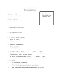
Uncertainties in Relic Density<br />
Bulk region: ˜B ˜B → Z, h → l¯l. Coannihilation: ˜τχ<br />
0<br />
1 → τ + X<br />
Figure 0: Bulk/coannihilation region. Full:<br />
SoftSusy, dotted: SPheno.<br />
<strong>SUSY</strong> <strong>Dark</strong> <strong>Matter</strong> <strong>and</strong> <strong>Colliders</strong><br />
B.C. Allanach – p.51/53
Focus Point<br />
Figure 0: Focus point region. Full: SoftSusy, dotted:<br />
SPheno, dashed: SuSpect. Higgsino LSP annihilates<br />
into ZZ/W W<br />
<strong>SUSY</strong> <strong>Dark</strong> <strong>Matter</strong> <strong>and</strong> <strong>Colliders</strong><br />
B.C. Allanach – p.52/53
High tan β<br />
BCA, Belanger, Boudjema, Pukhov, Porod, hep-ph/0402161. Baer et<br />
al<br />
Figure 0: High tan β region. Full: SoftSusy, dotted:<br />
SPheno, dashed: SuSpect. Get annihilation into A.<br />
<strong>SUSY</strong> <strong>Dark</strong> <strong>Matter</strong> <strong>and</strong> <strong>Colliders</strong><br />
B.C. Allanach – p.53/53