Using a Digital Oscilloscope for Signal Analysis - Teledyne LeCroy

WHITE PAPER
Using a Digital Oscilloscope for Signal
Analysis including a Practical Example of
PLL Characterization
Dr. Michael Lauterbach
Wayne Swirnow
LeCroy Corporation
The oscilloscope has been a primary tool for electronic design engineers
since the invention of that instrument, many years ago. The first decades
of oscilloscopes were “analog” in nature. Their fundamental technology
was the front end amplifier, sweep generator and—most particularly—
the phosphor which was used to coat the screen of a CRT. That phosphor
served as a memory element that briefly held the shape of the signal on
the CRT for the viewer. The value of the scope was in its ability to
trigger many times per second and overlay the phosphorescent images
on the screen. Information concerning the waveshape of the signal was
transferred via viewing the signal (sometimes using a hood to eliminate
light sources and at other times using a camera). The analysis was done
in the brain of the human who viewed the information and extracted
insights from the waveshape.
Back in the early 1980’s the analog oscilloscope began to give way to a
new type of instrument a for capturing and measuring signals called the
digital oscilloscope. The digital scope sometimes called the DSO
(Digital Storage Oscilloscope) offered the user the ability to capture a
waveform by converting the analog data to digital numbers, then
displaying the data points on the CRT screen. Because all the data was
now stored in memory there were several advantages to this technology
with regard to viewing and analyzing the waveform. Engineers who
were looking at single shot or low repetition rate events found that the
DSO provided a way to capture, store and view a very brightly displayed
waveform regardless of how slow the rep rate was. Also, the DSO did
not suffer from the waveform decay or blooming display issues which
were problematic with analog storage oscilloscopes. The DSO’s digital
format gave the engineer the ability dive further into analysis of the
waveform than earlier “viewing technologies.” New tools to perform
waveform measurements automatically like pulse parameters removed
subjectivity and variability caused by the engineer “reading the screen”
and increased measurement accuracy. There were feature sets like pre
and post trigger display, multiple zoom capability, and waveform
analysis such as averaging, basic math and FFT which the basic analog
scope simply could not do. These tools made waveform analysis
available to every engineer without the need to use standalone digitizer
cards and write software for analyzing the data.

Some applications are still best suited to use of oscilloscopes that can
quickly trigger and present of a view of the signal—using a time
constant that allows many signals to be overlaid on the screen
simultaneously. The fastest analog storage scope on the market today
can trigger up to 1,000,000 times per second and draw each individual
signal on the screen in real time, with a variable decay rate for the
phosphorescence. But the market for such scopes is dying away,
primarily because design/test engineers can no longer extract sufficient
information from a signal by viewing it. In many applications, “viewing
tools” are becoming a dead end. They take the engineer a short distance
in the right direction, but give no way to get where he really needs to go.
As an example, an engineer might be tasked with verifying the
performance of a 133 MHz clock used to transfer data to/from a microprocessor.
One key question is whether the clock meets certain test
standards for cycle-to-cycle jitter. Imagine an engineer trying to visually
observe 133 million cycles of the waveform per second on the screen
and trying to decide “by eyeball” if the clock meets the spec. Impossible.
Actually, if there is a gross error in the clock it could be obvious the
signal does NOT meet the test standard, but in the more normal case it
isn’t clear from observing a long, complex waveshape whether the
circuit is working properly (or not).
So here is the conundrum. How does a digital oscilloscope, which can
capture a large amount of highly accurate data—which contains the
answer the user needs—display that data in a way that extracts the
desired content concerning a complex signal structure. If the information
is that the signal “passes” a certain test standard, the scope could
simply display a text message. But if the circuit is not working properly,
how can the myriad information available in the scope be displayed in a
way that gives insight to the user This brings us to the concept of
“WaveShape Analysis” which is the ability of an oscilloscope to represent
complex data using a format which is NOT the usual voltageversus-time
waveform. The new view of the data should allow the
engineer to “discern by viewing” and “confirm by measuring” using the
new view of the data—just like he did in the “old days” by viewing the
raw signal shape and putting cursors on it to make a measurement. This
type of analysis is based on being able to view waveforms in the time,
frequency, statistical and parameter modulation domains. Only by using
this broad range of views can the oscilloscope user gather a complete
understanding of the circuit/device performance. WaveShape Analysis
involves the ability to use powerful math functions to transform signals
from one domain to the other. All of this processing has to be easily

accessible, understandable, and lightning fast, otherwise it will not be
used. Modern digital oscilloscope have finally matured to the point
where they can enable engineers to quickly acquire, measure, and
analyze and present to the user in simple to view formats vast amounts
of data. The scope can extract “information” from “raw data.”
The classic oscilloscope measurement provides a view of voltage as a
function of time. While this basic measurement tool has stood the test of
time, today’s complex signals require much greater WaveShape Analysis
capabilities than simple cursor or parameter measurements in order to
extract the useful information. Signals today are too complex to discern
if they are correct simply by looking at the mass of data on the scope
screen and it has become difficult confirm their behavior by measuring
using conventional parameters because many these parameters cannot
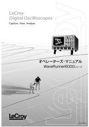
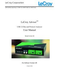
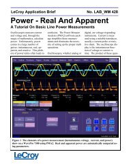
effectively or completely operate on long complex data sets. Figure 1
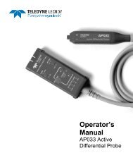
shows a simple but powerful example of WaveShape Analysis. Often,
the key characteristics of a signal are computed as pulse parameters such
as frequency, duty cycle or the timing skew between two edges. Early
digital scopes would simply display the latest measurement of the
parameters. Several years ago oscilloscopes began displaying statistics
including the high, low average and rms values of parameters. But the
user gets little insight into the source of circuit faults from these
numbers. They simply report if the signal meets or fails the specification.
A histogram is a new view of the parameter data. It is a bar chart
that shows how often each value of the parameter occurred. This new
view (a re-presentation of the data) allows simple viewing and easy
measurements tha t extract information from a complex set of raw data.
The “histicon” (icon size view of a histogram) of the frequency parameter
in Figure 1 shows the basic frequency is not stable—and the
“bathub” shape is an immediate indication that the frequency variation
is due to a sinusoidal modulation (for more information on interpreting
histogram shapes, there are application notes at www.lecroy.com). The
Gaussian shape of the duty cycle histogram means this parameter has a
central value which is being affected by noise. The skew between
channel 3 and channel 4 is a flat histogram. This indicates there is an
equal chance of timing skew, over a certain range of times, between the
two channels. The user gets immediate information from a straightforward
view of each distribution and furthermore can make simple
measurements. The most advanced oscilloscopes have very fast data
throughput that enables the display of up to eight simultaneous histicons
of any parameter.

Figure 1 Histicons (histogram icons) showing frequency modulation, noisy
duty cycle and a flat distribution of timing skew.
The ability to extract useful information from complex signals is further
complicated by the length of the waveform record. A few years ago a
DSO with real time or single shot sampling rate of 1GS/s was
considered reasonably fast. If a 1 GS/s scope, capturing one sample per
nanosecond, recorded a short simple waveform using 50 kpoints, the use
of a 20 GS/s scope (20 data points per nanosecond) will require 20 times
more memory, 1 Mpoint, to capture the same length signal. Of course
the newer scopes with higher sampling rates capture a signal much more
accurately and show more signal detail. But not only does the oscilloscope
now need to have much longer record length just to cover the
same time span but it also needs a high speed data path to handle this
long array and be able to perform calculations on a large data file.
Simply having long memory in an oscilloscope is not enough.
The challenge for T&M companies is to create a DSO with high
sampling rates, long memory and very specialized hardware/software
infrastructure which has been designed to acquire, move, process and
extract useful information from long complex data records. This process
must be fast, so the engineer is not kept waiting for the process to
complete, therefore usability of the instrument stays high and the
engineer stays productive. LeCroy has addressed this challenge through
the invention of new extremely fast, streaming architecture—named
X-Stream technology. The new technology makes measurements
10–100 times faster than previously possible, to allow more accurate
measurements, faster measurements and the ability to decrease deadtime
when making measurements (thereby increasing the likelihood of being
able to measure an intermittent fault). Let’s look at a practical example
of a moderately complex measurement—the characterization of performance
of a phase locked loop.

A Practical Example
of Analysis—
Characterizing
Performance of
a PLL
In Figure 1 the scope user sees a statistical domain view of signal
characteristics that gives insight into the waveform. A different type of
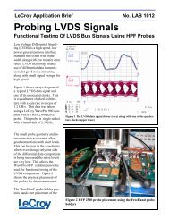
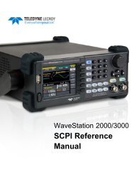
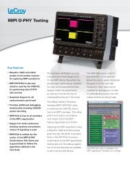
WaveShape Analysis, in the time domain is shown in Figure 2. The
acquired waveform is 200 usec long and is sampled at 8 Gs/s—
generating 1.6 million points of data. The signal in the upper half of the
screen is 100,000 cycles of a phase locked loop. During the acquisition
window, the PLL is “kicked” from a low frequency to a higher one.
While the upper trace presents the usual voltage-vs-time oscilloscope
display, the lower trace is a new presentation of the data. Every period
of the PLL is measured and the lower trace tracks the PLL frequency
(1/period for each of the 100,000 periods) versus time. The new view of
the data shows the frequency begins at a stable, low value then there is
a step which overshoots and settles to a new, higher frequency. We call
this trace a “JitterTrack.” It is easy to view the timing changes of a
circuit with this type of trace and to make measurements such as the
amplitude of the frequency shift (70.2 kHz), base/top frequencies
(9.638/10.0340 MHz), rise time of the frequency step (2.50112 usec)
and overshoot (62.32%).
The PLL response shown in Figure 2 is fairly simple. In general, the
output phase of a PLL will respond to changes in the input phase–but
only if those changes are within the bandwidth range the PLL. Input
changes that occur at low frequencies are passed to the output but high
frequency changes are too fast for the PLL to respond. An engineer will
often want to characterize the response curve of a PLL versus frequency.
This is sometimes called the PLL loop bandwidth, or the jitter transfer
function of the PLL. This brings us to a third type of view which can be
used to gain insight into circuit behavior—the view in the spectral/
frequency domain.
We can measure the PLL loop bandwidth by applying an input signal
that contains a step change in phase. This will allow us to measure the
step response of the PLL. The PLL impulse response can obtained by
differentiating the step response. The FFT of the impulse response is the
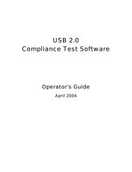
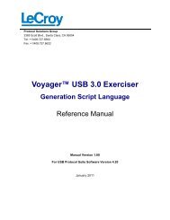
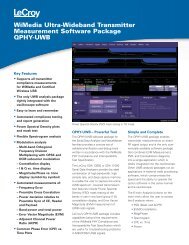
frequency response of the PLL. Figure 3 shows the measurement of
the frequency response of the input signal. The top trace (left side) is the
input reference signal—a 66.67 MHz signal with a 2 radian step in
the phase at the center of the trace. The JitterTrack (second trace on left)
of TIE (Time Interval Error) actually shows the step. This is a very
powerful WaveShape Analysis tool, “Parameter Modulation View”
taking the large and complex data set with a phase shift in the top trace
and re- presenting it in a simple to discern and measure processed trace.
We have just extracted very useful information from the input signal.

Figure 2 The upper trace is 100,000 cycles of a PLL. The lower trace is formed from a series of numbers
which track the frequency of the PLL. This JitterTrack presents a simple view of a step change in PLL
frequency. Parameters measure the characteristics of the frequency shift.
This is differentiated (third trace left) and then processed through an
FFT and averaging to show the frequency response of the input in the
bottom trace. This is the input excitation to the PLL and it is a spectrally
flat input out to 5 MHz (to within about ± 1.5 dB).
In Figure 3 (right half) the output signal is analyzed. Going through the
identical processing steps the result is the output response of the PLL.
Note that it is a lowpass characteristic with an upper cutoff frequency of
about 3 MHz. There is a broad peak at about 2.5 MHz, after which the
response rolls off. The final step is the divide the output spectrum by the
input spectrum as shown in Figure 4. As these are both logarithmically
weighted, this is the normalized frequency response of the PLL.

Input signal 66.67Mhz
Output signal
Time Interval Error
(Demodulated phase)
Demodulated phase
response
TIE differentiated
(impulse response)
2.5MHz
FFT
.5MHz/div
Figure 3 Input (left side) and output (right side) comparison of PLL”
This type of WaveShape Analysis can be extended to measure characteristics
such as phase offset between the input and output waveforms.
Measurements can be made for static clock frequencies or in the presence
of spread spectrum modulation.
All of the WaveShape Analysis we have applied has been derived from
the raw voltage vs time measurements of the input and output waveforms.
But, as in many applications, the user cares less about the raw
data and is more concerned with information concerning component/
circuit performance. These crucial performance characteristics can best

Output FFT
Input FFT
Output FFT/Input FFT
Figure 4 Frequency response of a PLL computed by taking the difference (bottom grid) of the logarithmic output and input
responses
be observed from waveform analysis in the time, frequency, statistical
and parameter modulation domains. Current oscilloscopes, which include
these highly integrated WaveShape Analysis tools more than pay for
themselves when it comes to solving problems involving today’s
complex electronic circuits and devices.
For more information on X-Stream technology, characterizing PLL’s,
and many other types of measurements, consult www.lecroy.com.