Full text - pdf - Peter Webster

UDC 551.613.1:551.511.33:551.509.313(213) 

Response of the Tropical Atmosphere 

to Local, Steady Forcing 

PETER J. WEBSTER ‘-Massachusetts 

Institute of Technology, Cambridge, Mass. 

ABSTRACT-A theoretical analysis is made of the largescale, 

stationary, zonally asymmetric motions that result 

from heating and the orographic effect in the tropical 

atmosphere. The release of latent heat dominates the 

sensible and radistional heating and the latter two effects 

are ignored. The first linear model is a continuous stratified 

atmosphere in solid westward rotation with no dissipation. 

Of all the modes, only the rotationally trapped Kelvin 

wave exhibits a significant response. Because the Kelvin 

wave response does not compare well with the observed 

flow, we concluded that the neighboring westerlies in the 

real atmosphere are important even if the forcing is in 

low latitudes. 

The second linear model is a two-layer numerical 

model including parameterized dissipation and realistic 

basic currents. Realistic forcing is considered, following 

an analysis of the response to especially simple forms of 

heating and orographic forcing. Dissipative effects close to 

the Equator are very important in this model. The dominant 

forcing at very low latitudes is the latent heating; at 

higher latitudes, the advective terms and the effects of 

rotation become more important and the influences of 

orography and heating are more nearly equal. A study of 

the energetics shows that the response near the Equator 

is due to both local latent heating and the effect of steady, 

forced motions at subtropical latitudes. 

Comparison of the response of the-model with observed 

motion fields and with the results of other studies suggests 

that most of the time-independent circulation of low 

latitudes is forced by heating and orography within the 

Tropics and subtropics. In the subtropics, however, 

forcing from higher latitudes must be of importance. 

1. INTRODUCTION 

During the last decade or so, the role of the tropical 

atmosphere in the general circulation has been a topic 

of great interest and some debate. Much of this debate 

has emanated from two differing theories as to how the 

tropical atmosphere is driven. The first avenue of thought 

centers on the idea that the lom-latitude condensation 

processes constitute the principal driving force of the 

tropical atmosphere (Riehl 1965, Manabe and Smagorinsky 

1967) , while the second theory considers lateral 

coupling with higher latitude energy sources as the most 

important driving force of the Tropics (Mak 1969). 

Charney (1969) suggested that a combination of both 

mechanisms is likely, and recently Manabe et al. (1970) 

reconciled the differences between the two theories using a 

numerical simulation study of the tropical atmosphere. 

From analyses of wind data in the lower stratosphere 

over the equatorial Pacific Ocean, the existence of transient 

planetary-scale waves were first identified by Yanai 

and Maruyama (1966). Since then, these transient modes 

have been the subject of many observational and theoretical 

studies (e.g., Matsuno 1966, Lindzen 1967, Mak 

1969, and many others). Except for the numerical study 

of Manabe et al. (1970), most investigations of the 

steady (or time-independent) circulations are of an 

observational nature. Kidson et al. (1969) studied the 

statistical properties of both the steady and transient 

large-scale equatorial motions using many years of conventional 

data. More recently, a detailed description of 

’ Now at the Gepartmcnt of Mrteorology, Unlversltg of California, Los Angeles 

the mean fields of motion at low latitudes for June, July, 

and August of 1967 has been undertaken by Krishnamurti 

(1970), who was able to supplement the conventional data 

coverage with aircraft wind observations. Other observational 

studies exist, but these tend to refer to some specific 

phenomenon in a specific region (e.g., the study of the 

easterly jet stream over the Indian Ocean by Koteswaram 

1958, Flohn 1964). With the exceptions mentioned above, 

the structure of the stationary circulations in low latitudes 

has received relatively little attent,ion. 

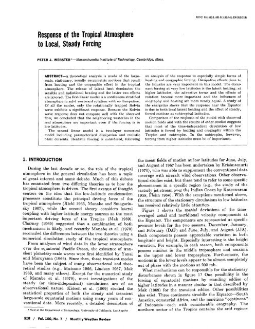
Figure 1 shows the spatial deviations of the timeaveraged 

zonal and meridional velocity components at 

the Equator. The components are represented at specific 

pressure levels for the two seasons, December, January, 

and February (DJF) and June, July, and August (JJA). 

Both components possess appreciable variation in both 

longitude and height. Especially interesting is the height 

variation. For example, in each season, both components 

possess minima in the middle troposphere and maxima 

in the upper and lower troposphere. Furthermore, the 

motions in the lower levels appear to be almost completely 

out of phase with the motions at 200 mb. 

What mechanisms can be responsible for the stationary 

disturbances shown in figure I One possibility is the 

forcing of equatorial motions by standing eddies of 

higher latitudes in a manner similar to that described bJ1 

Mak (1969) for the transient eddies. Other possibilities 

also exist. Three continents straddle the Equator-South 

America, equatorial Africa, and the maritime “continent” 

of Indonesia-each with considerable orography. The 

northern sector of the Tropics contains the arid regions 

518 I Val. 100, No. 7 / Monthly Weather Review

tn 

- 

5 

-5 

5 

-5 

E5 

-5 

5 

-5 

U' OJF U' JJA V' DJF V' JJA 

200mb 

400mb 

700 m b 

lOOOm b 

FIGURE 1.-Observed values of the spatial deviation of the timeaveraged 

velocity fields along the Equator for the two seasons, 

DJF and JJA. The zonal and meridional components (U' and V', 

respectively) are shown at the indicated pressure levels. 

Although such complicated feedback mechanisms may be 

incorporated into the model, it is a difficult and costly 

task to study one particular process or phenomenon. 

In the ensuing study, our philosophy will be to make the 

models simple enough for mathematical tractability 

while still retaining as many of the features of the tropical 

atmosphere as we can. The price we pay for this is the 

simplicity with which we must represent the forcing 

functions. For example, it will be necessary to introduce 

the orographic forcing as a simple boundary condition at the 

lower boundary of the model. Then, rather than allowing 

the motions to interact and determine the latent heat 

release, we are forced to seek the circulation that is consistent 

with a known forcing function. The problems 

involved in representing the forcing functions in this 

manner will be discussed in the next section. 

of the Sahara and the Middle East, the Indian subcontinent, 

and the Himalayan Mountains. The annual 

distribution of precipitation in the Tropics reveals a 

large longitudinal variation. For example, each of the 

three tropical continents possesses relative precipitation 

maxima, the possible importance of which has been 

discussed by Ramage (1968). It thus seems that the 

orography, the release of latent heat, the effect of the 

ocean-continental contrast, and perhaps a longitudinal 

radiational heating variation could play a role in the 

production of the standing eddies. The purpose of this 

study is to assess the role played by these forcing functions 

located within the Tropics. 

Specifically, this study is a theoretical attempt to 

investigate the large-scale, stationary, zonally asymmetric 

motions that result from the influence of forcing 

functions within the tropical atmosphere. The importance 

of forcing from higher latitudes is also discussed. 

In midlatitudes, the study of steady motions generated 

by longitudinally dependent forcing has a long history 

going back at least to Rossby's (1939) surmise on the 

excitation of the free modes of a simple atmosphere. 

Charney and Eliassen (1949) were the first to make a 

detailed study of the perturbation of the westerlies by 

orography. They were soon followed by Smagorinsky 

(1953), who considered the effect of zonally asymmetric 

external heating. Since these pioneering works, there has 

been a multitude of similar steady-state models that have 

been fairly successful in reproducing at least the gross 

features of the midlatitude stationary flow. 

The above studies were all steady-state linear boundary 

value problems. A second form of model instigated by 

Phillips (1956) consists of starting with some prescribed 

initial state and predicting its evolution over a long period 

of time. The time-averaged solution is considered to be the 

climate of the model. Such models have become very 

sophisticated and now extend over the entire globe and 

include many levels in the vertical. The numerical methods 

of solution allow the incorporation of various physical 

processes such as the release of latent heat through a 

complete hydrology cycle (e.g., Manabe et 81. 1970). 

2. FORCING FUNCTIONS AT LOW LATITUDE 

Since the topography of the earth's surface is well 

known, the determination of the orography function 

presents little problem. The resolution of the heating 

functions, however, is a much more difficult task. Such 

functions cannot be measured directly; therefore, a 

relationship between the function and some other observable 

field(s) must be known. Even if we know the relationship 

well, we have to cope with the observational problem, 

which is especially acute in equatorial regions. To overcome 

this observational problem, we will make use of 

satellite data to determine at least the gross features of the 

major low-latitude heat sources and sinks. 

Being primarily interested in the response of the 

tropical atmosphere to localized forcing, we will assume 

that the forcing functions decay exponentially poleward 

of 30° latitude according to the lam 

f(e)=exp [-1O(sin e-o.3)2] (1) 

so that orographic or heating functions, x(e,cp), may be 

written as 

x(4 cp)=x(4 cp) le1 530" 

and 

x(eJ cp)=x(e=300, V)f(e) le 1 > 30 O. 

(2) 

The reverse problem, that of the influence of steady forcing 

from midlatitudes upon the tropical region, mill be discussed 

later. 

Orography 

To form the orographic function, we used the estimates 

of Berkofsky and Bertoni (1955). From their 5" average 

elevations, values every 10" of longitude and 5" of latitude 

between f 30" latitude were extracted. This produced 

the array h(e,V). 

The orography function is conveniently represented 

in wave-number space. To do this, we expand the orography 

in the Fourier series 

h(0, p)=C [&((e) cos scp+h;(e) sin scp] (3) 

s=o 

July 1972 1 Webster / 519

180.W 

TABLE 1.-Zonal mean and zonal rms values of the various heating 

functions (calern-2day-1). Calculations were made using the 

estimates of Katayama (1964) 

Lat. 00 10°N WN 30"N 

RAD -210f 12 

SEN 61 24 

9 " 288-f 110 

9 TOTAL 83f 112 

9 RAD -192f 19 

9 SEN 1Of 18 

9 LH 256f 112 

9 TOTAL 74 f 108 

January 

-255k 25 

7f 22 

196f 111 

-18f 113 

July 

-183& 24 

llf 28 

354f 139 

185f 152 

-238rt 24 -216% 26 

26f 20 39f 24 

83% 80 118% 80 

-1OOf 88 -35f 95 

-185% 23 -175f 27 

32f 40 63f 55 

232f 192 157f 166 

88f 198 57f 180 

FIGURE 2.-Composite map of (A) thc orography (lo2 m), (B) the 

DJF latent heating (10-2 cal.cm-2.day-1), and (C) thc JJA latent 

heating using the first nine nonzero Fourier coefficients. 

where hX(0) and h:(@ are the real sth cosine and sine 

coefficients, respectively, and s is a non-negative integer. 

Figure 2A illustrates the recomposition of the orography 

with the first nine harmonics, except s=O. Four 

features predominate. These are the Andes, the African 

highlands, the mountains of the maritime continent 

Indonesia, and the Himalayan Mountains. In forming 

the orographic forcing function, we will only use the 

first nine longitudinal l~armonics, as the inclusion of the 

higher wave numbers teiids only to "sharpen" the existing 

peaks and "smooth" the surface of the ocean. 

Heating 

Heating and cooling of the atmosphere involves many 

complicated processes. In the simplest sense, we may 

represent the total heating in a unit column (cal.cm-2.day-') 

as 

9 TOT&= (9 sw+ 9 Lw) + 9 BEN+ 

9 LH 

where 98w represents the absorption of solar short-wave 

radiation in the column, gLW is the long-wave emission, 

gSEN is the heating or cooling by the turbulent transfer 

of sensible heat between the atmosphere and its lower 

boundary, and QLH is the heating or cooling due to the 

condensation or evaporation of water vapor. 

The complexity of investigating the heat budget of 

the earth-atmosphere system or estimating those heating 

functions likely to be of importance in our study is 

cxernplified by the interdependency of the various terms 

in eq (4). For example, the large release of latent heat in 

the tropical atmosphere is likely to be dependent upon, 

(4) 

at least initially, an equatorial flux of moist air forced by a 

mean north-south radiation heating gradient. Also, the 

preferred longitudinal distribution of precipitation in the 

Tropics (and hence the release of latent heat) appears to 

be coupled to the sensible heat flux at the lower boundary. 

An example of this interdependency is the cloudless region 

of the equatorial southeastern Pacific Ocean that coincides 

with the cold oceanic upwelling areas. 

Unfortunately, the linear aspects of our study do not 

allow the treatment of the interdependency and full complexity 

of the terms in ecl (4). Rather, we can, at best, 

treat these processes as separate entities and estimate 

their relative importance. To do this, we will utilize 

earlier atmospheric heat budget studies. 

From Katayama (1964), we have mean estimates of the 

terms of eq (4) for January and July over the Northern 

Hemisphere. Using these results, the zonal average and 

root-mean-square (rms) value of each term was calculated 

at Oo, 10"N, 2OoN, and 30°N for both months. The 

results are displayed in table 1. 

Considering the rms values of the various terms, we 

note that the longitudinal variation of 9 RAD (where 

9 RAD= 9 8w+ 9 Lw) and 9 is appreciably smaller 

than 9 In fact, latent heat accounts for nearly all the 

total variance. Thus, in choosing the most important 

terms of eq (4), we must relegate the longitudinal variation 

of 9 and 9 RAD to a position of secondary importance, 

both individually and cumulatively, in comparison 

to 9 Ln. 

Distribution of Latent Heat 

Because most estimates of the distribution of the release 

of latent heat utilize an observed distribution of precipitation 

(e.g., Katayama 1964), one must devise an alternative 

method of determination for the Tropics that shows 

no bias between oceanic and continental regions. 

In an attempt to achieve this goal, we assumed a direct 

relationship between cloudiness and precipitation (and so 

latent heat release). Some credence is given to this 

assumption by Johnson (1969), who found a high correlation 

between the average precipitation and cloudiness over . 

520 1 Vol. 100, No. 7 1 Monthly Weather Review

a region of Bangladesh (formerly East Pakistan) during a 

3-mo period of the 1967 monsoon season. Estimates of 

cloudiness were obtained from the digitized ((brightness” 

or mean global, visual, albedo satellite charts compiled by 

Taylor and Winston (1968). To allow the brightness 

charts to be representative of cloudiness, we first delineated 

the bright cloudless areas over the desert regions using 

climatological data. Such areas were relegated to the lowest 

brightness index. We evaluated the factor of proportionality 

by correlating the zonal average cloudiness with the 

zonal average of the latent heat release from Katayama 

(1964). Thus, an error in Katayama’s estimate obtained 

from conventional data results only in an error in magnitude 

and not in distribution in our heating function. 

In the above determination, we assumed that the background 

albedo of the land and ocean surfaces is the same. 

However, Budyko (1955) estimates that the albedos are 

approximately 7 percent and 15 percent, respectively, 

thereby slightly overestimating the latent heat release 

over land. Correcting for this error is a dillicult task. One 

cannot simply reduce the latent heat estimates over land 

by some appropriate amount without equally affecting 

areas where the background reflection is unimportant, 

such as areas of high mean cloudiness. 

Following the same procedure as with the orography 

function, we expand the latent heating field in the Fourier 

series 

9 LH(e,cp)=~ s=o [*:(e) cos scp+a;(e> sin 8.1 (5) 

where qi and q; are the sth real sine and cosine coefficients. 

Figures 2B and 2C represent the recomposition of the 

seasonal latent heat distribution using the first nine 

nonzero coefficients of eq (5) and comprise spatial deviations 

(or perturbations) about the zonal mean. In DJF, 

three large maxima are apparent; these correspond 

roughly with the equatorial regions of South America 

(particularly the Amazon Basin), southern equatorial 

Africa, and the Indonesian region. [Ramage (1968) 

discussed the importance of the tropical continents as 

major sources of latent heat.] Arid North Africa and the 

Middle East appear as negative anomalies (or relative 

cooling regions) as do the southern Atlantic Ocean and the 

southeastern Pacific Ocean. Considering the JJA recomposition, 

we note the dominance of the extremely 

strong heat source in the vicinity of the Indian subcontinent. 

Relatively weak maxima are to be found in 

Africa and in the north and central parts of equatorial 

South America. 

The southwestward extension of the latter maximum 

underlines a possible weakness in the scheme used to 

evaluate QLH. In assuming that a direct proportionality 

exists between cloudiness and latent heat release, we have 

made the tacit assumption that cloudiness is proportional 

to precipitation. This assumption is perhaps better in the 

tropical atmosphere than elsewhere as cumulus is the 

predominant cloud type. However, from climatological 

precipitation data, the region mentioned above is particularly 

dry and the relatively high QLH value is a result 

of persistent nonprecipitating cloud cover. 

The latent heat distributions will enter the equations of 

our models as steady-state or time-independent heating 

functions. But should one interpret the functions as constant 

regions of relative heating On a day-to-day basis, 

we find that most precipitation results from transient disturbances 

of various time and space scales. More correctly, 

then, we should think of the latent heat fields as the timeaveraged 

effect of these disturbances. 

How much confidence may we have in these estimates 

To test them, we compared selected areas of relatively 

well-known precipitation distribution with the seasonal 

latent heat determinations. The calculations, summarized 

in appendix 1, result in fairly good agreement between the 

implicit and ex phi t de termin a tions. 

3. SIMPLIFIED CONTINUOUS MODEL 

In this section, we will consider a simple linearized model 

that retains some important features of the real atmosphere. 

To facilitate separation of the basic equations, we 

chose a mean state in which the basic zonal flow is one of 

solid rotation. That is, we let 

U( e) = ~ UQ sin e 

(6) 

where e represents colat.itude, 6 is some nondimensional 

number, a is the radius of the earth, 0 is the angular 

velocity of rotation of the earth, and 77 is the basic zonal 

flow. For a westward flow of 5 m/s at the Equator, 

6=-10-2. The mean temperature is allowed to vary 

only with height, and both the basic and perturbation 

states are assumed to be hydrostatic. For simplicity, radiational 

and frictional dissipative effects are ignored. 

Governing Equations 

The governing equations arise from the spherical 

primitive equations in (e, ‘p, Z=ln p/po) coordinates as 

given by Phillips (1963). Here, p represents pressure, 

p, is some constant, and cp is longitude. The solutions are 

linearized about a basic state defined by eq (6). Assuming 

steady-state solutions (Le., a/at=O), we derive the following 

linear set: 

1- 

2Q COS e+- U cot 0 

a 

where K= 

The 

symbols u, v, and 2 represent the zonal, meridional, and 

vertical components of the perturbation velocity field, 

and $ and are the perturbation and mean geopotential 

heights, respectively. 9 is the heating rate per unit mass. 

RIG, and “(2) = (a,@Z) [aT/aZ+ (KF)]. 

July 1972 / Webster / 521

The longitudinal variation is separated out by assuming' Then, between eq (13) and (14), we can separate eq (11) 

that 

yielding the vertical structure equation, 

and 

-iW, W(0, 2) exp (isp) (84 

Me, 'PI, 928, 'P, Z)=RIChs(e>, as(& 2) exp (~s'P) 

8 

(8b) 

where h'=h;-ih~ and q8=&-iq; via eq (Sb), (3), 

and.(5). The term, 8, is a Don-negative integer, i2=-1, 

and R1 signifies the real part of the expansion. 

Noridimensionalizing, using a and (23)-' as the length 

and time scales, and introducing eq (8) into eq (7) produces 

the following linear relatiopships between the coefficient 

functioas of p, 2, and s. These are 

and 

- Xsu" + ApV + SY = 0, (94 

-XsVs+ApUs+D(sS) =O, 

--sUS+D(V)+(l -p2)P(WS)=O, 

iwxs 

,,+E(Z)W=n"(r,Z) 

(9h) 

(9c) 

(9d) 

where p=cos 8, D= (1 -pz) (a/&), P= (a/aZ) - 1, A= 1 +S, 

and 

X,= - 6J2. (10) 

The term, X, the apparent or "Doppler-shif ted" frequency 

of the motions (i.e., the frequency of the various modes 

referred to a frame moving with the baeic current), is 

positive for easterly flow (60). 

By straightforward elimination, eq (9) is reduced to a 

single second-order equation in W(p,Z). That is, 

where 

and 

m( p) =A: - A2p2. 

3, the "traditional" Hough operator, is shown by Flattery 

(1967) to be self-adjoint, which infers its possession of 

real eigenvalues and orthogonal eigenf unctions. 

If W:,$ is the nth eigenfunction of 3 such that 

where the En,s are the associated eigenvalues, we can 

expand W(B, Z), ~J(M), and ps(p, 2) in these eigenfunctions. 

That is, 

wS(p, z), P~((CC, Z>, hJ(p)=XPn. s(z>, Jn, s(Z>, 

522 / Vol. 100, No. 7 / Monthly Weather Review 

bn, swE..s(~>. 

(14) 

Eigenfunctions and Eigenvalues 

The problem is to find W:,s(p). We do not seek its 

general form, however, but only that form defined by 

- the parameters of our very specific problem. These are 

U (and hence 6) and s, which together define A,. In 

appendix 2, we shorn that these parameters define specific 

ranges of magnitudes for the eigenvalues that are then 

used to obtain the appropriate forms of W:Jp). 

The Free Regime 

An investigation of the free regime allows us to anticipate 

the reaction of the model to forcing. Similar discussions 

have been given for the E>>O free modes by 

Matsuno (1966) and Lindzen (1967). Our approach differs 

in that we seek only to illuminate the forcing problem. 

The latitlxdinal equation [eq (45)] represents four modal 

families. These modes are, respectively, a set of westward 

propagating Rossby waves, R, easterly and westerly propagating 

gravity waves, GE and GW, and an eastward 

moving Kelvin wave, K. In an eaeherly basic flow, only 

the eastward propagating GE and K modes are capable 

of being excited by stationary forcing functions. R and 

GW are thus ignored. A summary of the properties of the 

remaining stationary free modes is given below. 

1. For an isothermal atmosphere and any realistic value of s(Z), 

ma in eq (16) is positive due to the large size of E. This means that 

all free solutions of eq (15) are vertically propagating waves and 

m may be considered to be the vertical wave number of the mode. 

2. The vertical wavelength (defined by 2rr/m) of all the GE 

modes is extremely small and varies from the order of a meter for 

small s to the order of a kilometer for large s. The vertical scale of 

the Kelvin wave is about 1.5 km for all s. 

3. The latitudinal scale of the GE modes [defined as the point 

where the solution of eq (45) changes from oscillatory to exponentially 

decaying; i.e., pc=A-l/2E-l/4 (an+ ])*/a] falls within a degree or 

so of the Equator. Furthermore, one can show that, for a given s, 

a limiting critical latitude (pc=Xs/A) exists as n+m. The e-folding 

scale of the symmetric Kelvin wave is f 7' of latitude. 

Because of the limited latitudinal extent of the E>>O 

eigenfunctions, they cannot represent the response of the 

tropical atmosphere at any distance from the Equator. 

The remainder of the representation must lie with the 

eigenfunctions associated with the negative eigenvalues. 

These functions possess maxima in the vicinity of the 

poles and, for the range of negative eigenvalues defined by 

our problem (Longuet-Higgins 1968) , decrease slowly in 

amplitude equatorward. However, in representing the 

basic state of the atmosphere by a simple easterly flow 

everywhere, we are making the tacit assumption that the

forcing functions, and hence the response, can be nearly 

represented by these modes having small amplitude at 

high latitudes. Since we need to consider the eigenfunctions 

for EO family at very low latitudes, it mill aid US in 

the interpretation of subsequent results of the more cornplicated 

model. The response of the GE mode will be 

ignored since, in addition to the properties mentioned in 

items 2 and 3 above, its magnitude is at least two orders of 

magnitude smaller than that of the Kelvin wave in the 

small to moderate s range. 

180‘W 90. w 0’ 

____-___ .- 

- -_ __- 

FIGURE 3.-~ertical cross-section along the Equator of the perturbation 

zonal current response (m/s) of the Kelvin wave due to 

forcing by the DJF latent-heat forcing function shown in figure 2B. 

The Kelvin Wave Response 

The Eelvin wave solutions are given by eq (53) and 

(54), subject to the appropriate boundary conditions. At 

2=m1 we insist that all energy is outgoing while, at Z=O, 

the boundary condition is given by the linear relationship 180.W 900 w 0‘ 

FIGURE 4.-Same 

as figure 3 for the JJA latent-heat forcing function 

shown in figure 2C. 

By introducing eq (8), (14), and (16), we can show that 

A 

Yn.s(Z=O) =xsbn,s (17) 

where the in,, represent the complex conjugates of the 

coefficients of eq (14). 

A maximum latent heat release near 5 km, in keeping 

with the determinations of Vincent (1969) , is obtained by 

choosing a functional form of f(2)=2 exp(--1.62 2). 

Using eq (5), (9), and (14), we may write the heating 

function as 

2.5 

t 

kr 

0 


900 w 0 4 90°E 

as figure 3 for the orographic forcing function 

shown in figure 2A. 

where the in,, are the complex conjugatfs of the, coefficients 

of .eq (14). The coefficient families, bn,,y and qn,,, are 

found from the transform of eq (14). 

Using eq (17) and (18), we can determine the solutions 

of eq (15) for the Kelvin wave response to orography (no 

heating) and thermal forcing (no orography). They are, 

respectively, 

Substituting eq (19) and (20) into the eigensolutions [eq 

(53) and (54)], plus the expansion coefficients of the three 

families of forcing functions, gives the three-dimensional 

response of the Kelvin wave. Figures 3-5 show crosssections 

of the perturbation zonal velocity response to 

the DJF and JJA seasonal heating and orography, 

respectively, along the Equator. 

The fields of figures 3 and 4 are both characterized by 

regions of converging and diverging zonal currents associated, 

respectively, with ascending and descending air 

over the heat sources and sinks. Since V=O, the resulting 

flow consists of zonal or longitudinal circulations in the (p, 

2) plane with riing motion in the western parts of the 

ocean and subsidence in the east. This flow pattern corresponds 

to the circulations discussed by Bjerknes (1969). 

Above this region, the response changes to one characterized 

by a vertical circulation scale on the order of a 

kilometer. This corresponds to the internal gravity part 

of the solution. 

July 1972 1 Webster 1 523

Comparing these results with figure 1, one sees some 

similarity in the lower levels where the westerlies centered 

near 90°W, 20°E, and 90°E are roughly simulated, although 

the strong westerlies near 140°E in JJA are not 

predicted. At higher levels, the observed phase change is 

not apparent. 

The most outstanding feature of the orographic forcing 

(fig. 5) is the magnitude of the response. As we shall see 

later, this is due to the neglect of dissipative processes in 

the model. The importance of dissipation to the steadpstate 

structure of the tropical atmosphere will becoine 

apparent when we compare these results with those of the 

more complicated model. 

4. FORMULATION OF A MORE REALISTIC MODEL 

To facilitate the study of the response of a more complicated, 

spherical, and hydrostatic basic atmosphere, 

we formulated a two-layer model. Such a model represents 

the simplest prototype of the atmosphere capable of 

possessing both horizontal and vertical shear in the basic 

state. The complexity of the basic fields and the numerical 

techniques needed to solve the equations make it a 

difficult task to employ a radiation condition at the upper 

boundary. We will assume that the upper boundary is 

rigid, although at this stage we must question the validity 

of such an approximation. 

As shown by the quasi-geostrophic considerations of 

Charney and Drazin (1961), the rigid lid condition is 

considered to be a good approximation when modeling 

midlatitude tropospheric motions. However, in low latitudes, 

these arguments are not valid. In a recent study of 

the maintenance of the quasi-biennial oscillation, Lindzen 

(1970) found that at certain levels the vertical propagation 

of equatorial waves was impeded. At such levels, the 

phase speed of the waves matched the basic flow. For 

time-independent waves (zero frequency), such critical 

levels occur where basic flow is zero. If such a surface did 

exist in the basic tropical atmosphere, it would provide 

an appropriate location for our rigid lid and would somewhat 

justify its inclusion. From the 6-yr zonal averages of 

Kidson et al. (1969), there appears to be little evidence of 

a zero surface at low latitudes; there is, instead, easterly 

flow through the stratosphere. However, as we will show 

in section 5, the importance of frictional dissipation in 

low latitudes suggests that for steady motions the assumption 

is inconsequential. 

Another feature of our two-layer formulation is the 

simplification of the basic stratification. First, the stratification 

is allowed to be a function of height only, thus 

being represented by one value at the midpoint of the 

model. Second, as a consequence of the assumed horizontal 

independence, one must be satisfied with a mean horizontal 

static stability. From Dickinson (1969, fig. 4), we see that 

the last assumption is fairly good; there is little variation 

of the static stability at 500 nib between 30°N and 30's. 

(Thompson 1961) are linearized relative to a basic state 

defined by 

- 

U P , P)=(1-cc2)'/2afwP, PI (21) 

where 6(p, p) is some nondimensional function to be 

determined. 

Introducing a, (an)-' and po=lOOO mb as the length, 

time, and pressure scales, we derive the following linear, 

hydrostatic, and spherical primitive equations: 

- pv' (2A f 1) = -- a$ + ( 1 - p2) '/'F,+,, (22a) 

a, 

where A(p, p)=6/2, ~'=(l-p~)~/~u, ~'=(l-p~)~~~v, and 

w = d p/d t . 

The two-layer model is schematically summarized in 

figure 6. The lower troposhere is represented by the fields 

at 750 mb and the upper troposphere by those at 250 

mb. The real tropical atmosphere, on the other hand, is 

more complicated than this as can be seen from figure 1. 

For example, the flow at 200 mb is not representative of 

the upper troposphere. Thus, rather than thinking of the 

results of the model as representative of a particular level 

in the atmosphere, they should more correctly be thought 

of as representing the average conditions of the layer. 

At the upper boundary, we set w=Q, while at the 

earth's surface, we assume that w=wc(p, p), a known 

function. The subscript G infers that the quantity is 

evaluated at the lower boundary. We also assume that a 

quantity evaluated at the interface of the two layers is 

the mean of the quantities evaluated at levels 5 and 2. 

That is, 

where the subscript denotes the level to which the variable 

applies. Then, using the upper and lower boundary conditions, 

we may approximate the vertical advection terms 

by 

and 

Governing Equations of the Two-Layer Model 

The nonlinear spherical equations in pressure coordinates 

where Ao= A(p= 1) 

524 / Vol. 100, No. 7 / Monthly Weather Review

p=l 

!J=O 

appropriate form of eq (22) is reached in the following 

manner. The momentum and continuity equations are 

expressed at levels 1 and 2, and the thermodynamic 

equation is given for the interface (p=%). After using the 

continuity equation to eliminate w and with eq (24), (25), 

and (7), we finally arrive at a set of equations in the 

p-dependent complex Fourier coefficients. These are 

Is( B+2C)-iK2]Us-;[CD.-Alp+D(B+C)]V;+iKz~ 

u=-1 

= -sq, 

A,pn+ i[s(B+ C)--iKz]V~--KzR=--D(q:), 

i&fl+i[CD+A,p-D(B+ C)]R+ (sB-iKi)E 

p=o 

w = o 

0 MB 

= -s*;--F;(p), 

AzpE-Kzfl+ i[~( B- 2C)-iKz]R=--D(%P@, 

sn +sic&- iD( Tq) - iD( Vi) =e( 

p) , 

and (27) 

fl-i [" D-C(1+2B)p %+iC(1+2B)pR 

(1--P2) 1 -p2 1 

1/2 w , s 500 MB 

1 1000 MB 

w 

= &IG 

FIGURE 6y-The 

two-layer model. 

We will assume the following simple linear dissipation 

laws (Charney 1959) : 

and 

F1(p,(P)= - ~z(V,-~z) (1-Pz)"2, 

FZ(~,(P)=[KZ(V~-V~)-K~VZI(~-P~)~'~, (25) 

$(p,(P)= 9 (p,(P)+K3(h-&l). 

Here, K,, K,, and K3 are representative of a surface drag 

coefficient, a coefficient of small-scale exchange of horizontal 

momentum vertically between the layers of the 

model, and a radiational cooling coefficient, respectively. 

g(p, cp) is the known heating function. The values me 

will use in all our calculations are K,=0.0308, K2=0.00343, 

and K3=0.00206 (Charney 1959). The value of wG is 

determined by using the approximate condition that 

where h(p,cp) is the nondimensional 

defined by 

(26) 

orography function 

The longitudinal dependency is separated out by expanding 

the variables in Fourier series as in eq (7). The 

469-748 0 - 72 - 2 

where B=(Al+Az)/2, C=(Al-Az)/2, and Aj=2Aj+1 

where 3=1, 2. B and C represent the barotropic and 

baroclinic parts of the basic zonal flow, respectively. 

The forcing functions, F:(p), are defined by 

3': (p) = - is( 1 -p')A,( A1 + A,- 2A G)~S (/A), 

E(p)=2is( 1-P2)AchS(P), 

and Fi(p)=- P(p). (28) 

For simplicity of notation, the s superscript will henceforth 

be understood. 

Numerical Method 

The numerical procedure used to solve eq (27) is 

similar to that used by Mak (1969). Rather than following 

the usual procedure of first reducing the set of equations 

to the simplest possible form, we initially expanded 

eq (27) in finite-difference form and then reduced. This 

precludes the problem of handling very complicated 

operators resulting from the p-dependent coefficients. 

The finite-diff erence scheme chosen is a one-dimensional 

version of the "staggered centered-diff erence" scheme 

described by Phillips (1962). The resulting six first-order 

cliff erence equations are reduced to two linear, complex, 

second-order, coupled difference equations by a relatively 

straightforward procedure. 

Following the procedure outlined in appendix 3, we 

derive two linear, complex, second-order, coupled difference 

equations. These are 

p:v:+ 1+p,kv: +py: -' +p,"vz" + ' +ptvt +p,"v,k - 1 

=rf+r;+rt+rt+rk+r," 

and (29) 

qkVk+' 

1 * + qz" v:: 

+ q3" v: - ' + q: vi +I+ nj" v; + qa: vz"- ' 

= t:+ t;+ ti+ t:+ t.k+ tG" 


where pi" and aj" are complex coefficients and rt and ty are 

the complex nonhomogeneous coefficients. The coefficients 

have the following functional form: 

and 

pf, pi"=jn(,,s,8,B,C,Kl1K~,K~,F~,F~,F~) 

rf, t: = jn(p, s,B, B,C,K~,KZ,K,,F~,F,,F,). 

Equations (29) are separated into real and imaginary 

parts providing a set of four real, coupled difference 

equations. 

To cover the latitude zone between the two poles, we 

used 41 gridpoints (k=l, 41 with Ap=0.05). The advantage 

of the cosine of colatitude as the latitudinal coordinate 

is here apparent since half the gridpoints in the p- 

space (-1, 1) lie between 3~30". Expressing the set of 

real difference equations at each point in the range, we 

arrive at a system of 4x39 (156) hear simultaneous 

equations in 164 unknowns. The balance of the unknowns 

is provided by the boundary conditions at the poles, 

which are 

v/ - 1 = v/ 41 = 0 

v; = 1 = vz = 41 = 0. 

and (30) 

The system of equations may be expressed in the matrix 

form 

A*X=F (31) 

-1 0.5 

1-10 

r 30 

L-lo 

**----- 

,- 

FIQURE 7.--The three basic zonal wind distributions (m/s) for 

DJF, JJA [from Vincent (1969)], and the symmetric annual field, 

ANN. The curves represent vat 250 (solid) and at 750 mb (dashed) 

where A(pjk,qjk) is the 156 X 156 coefficient matrix 

X(V,",Vt) is the 1 X 156 variable matrix, and F(~jk,tfk), is 

the 1 X 156 nonhomogeneous matrix. Fortunately, the 

matrix is banded (ise., consists of a main diagonal and 

Seven adjacent upper and Seven adjacent lamer diagonals, 

while the remainder of the terms are zero), the 

use of a fast numerical L ' G eliminationl> ~ ~ ~ ~ method 

(International Business Machines 1968) to invert eq (31). 

The Basic Fields 

The basic zonal wind fields were obtained from Vincent 

(1969) and are shown in figure 7. Three basic fields are 

used. The first two are the seasonal averages for DJF 

and JJA. The most apparent features are the large horizontal 

and vertical shears within the Tropics. For example, 

in the winter hemisphere of DJF and JJA, large shears 

exist at quite low latitudes. 

The third field, an idealized approximation of the annual 

mean wind field (labeled ANN), is given by t'he 

expressions 

- 

3* 

U1(p)=18 sin - (p+1)+14(1-p2) 

2 

and (32) 

- 37r 

U2(p)=7 sin (p+l)+2(1--p2)- 

ANN will be used to consider the response of the system 

to hypothetical forcing functions. 

We found two possible distributions of the basic zonal 

velocity at P=l for the model. The first, a linear extrapolation 

of the basic wind field to the ground, produces 

very strong easterlies at P=l in regions Of strong shear in 

midlatitudes (e.g., at p=0.5 in DJF). In better agreement 

with the observations is the assumption that 

(33) 

For the static stability, we found that B=0.0083 best 

represents the annual mean static stability at 500 mb 

between 130" of latitude. This value is approximately 

the same as that used by Mak (1969). 

5. RESPONSE OF THE TWO-LAYER MODEL 

In an attempt to approach an understanding of the 

manner in which a basic state containing both horizontal 

and vertical shear will react to the complicated forcing 

fields, we will consider some illustrative examples. 

Specifically, we will consider the reaction of the hypothetical 

symmetric basic state ANN to the placement 

of the idealized energy sources at specific locations. 

Following this, me will consider the response of the DJF 

and JJA basic fields to the combination of thermal and 

orographic forcing, and finally we mill compare the 

predicted motions with some observed values. 

It is interesting at this point to anticipate what may 

be the important physical processes governing the 

526 1 Vol. 100, No. 7 f Monthly Weather Review

esponse of the model in low latitudes. During the description 

of the model, we discussed the incorporation of 

dissipative mechanisms. The values chosen for the effects 

of surface friction, the small-scale exchange of horizontal 

momentum, and radiational cooling provide decay times 

of approximately 6, 25, and 40 days, respectively. Near 

the Equator, the magnitude of the basic current is about 

5 m/s. This provides an advective time scale (defined 

in our model as the time required for a parcel to be 

advected by the basic current over one longitudinal 

wavelength) for the longest longitudinal scale (s= 1) on 

the order of 80 days. For s=2, the time scale reduces to 

40 days, and so on. By comparing the dissipative time 

constants with the advective time scales, we can expect 

that the dissipative effects will be very important for 

equatorial motions. As we move into the westerlies, the 

advective time scale will be much smaller because of the 

increase in magnitude of the basic current and decrease 

in the circumference of the earth. Consequently, frictional 

effects will be less dominant. 

Response to Idealized Forcing 

The basic field, ANN, will be forced by a distribution 

of heating or orography of the form 

l800W 9oow 900E 18O'E 

FIGURE 8.-Distribution 

of heating (102 cal.cm-2.day-l) or orography 

(km) for (A) p.=O and (B) ~~'0.4 for the hypothetical 

forcing fields given by eq (34). 

to provide a function that is symmetric about the prime 

meridian and some latitude p=pc and e-folds within 

540' of longitude and f12" of latitude. For a heating 

function, me chose A=600 cal.cm-2. day-', while for the 

orographic case, we let A=6000 m. The amplitudes of 

the function were chosen to correspond to the amplitudes 

of the heating over India in JJA and the Himalayan 

Mountains, respectively. Figure 8 shows a recomposition 

of the Fourier expansion of eq (34) with pc=O and 0.4, 

using the first nine nonzero Fourier coefficients. 

Response with pc=O. Figure 9 shows the perturbation 

horizontal velocity and height fields due to the hypothetical 

heat source centered at p=O and cp=r. The effect of a 

similarly located orographic function is shown in figure 10. 

We mill consider the heating function first. Both 

velocity fields (250, 750 mb) are characterized by strong 

* . . 

750 m b 

FIGURE 9.-Horizontal perturbation velocity (vectors) and geopotential height deviations (solid lines) of the basic field, ANN, at 250 and 

750 mb in response to an isolated heat source given by eq (34) with pc=O and A=600 cal.cm-2.day-'. The vector magnitude is proportional 

to the indicated scale and the geopotential heights are in meters. 

July 1972 Webster f 527


750 mb 

as figure 9 for orographic forcing given by eq (34) with pC= 0 and A=6000 m. Note that the vector magnitude scale has 

been increased by a factor of four. 

zonal currents located along the Equator flowing into the eq (16), which together with eq (50), may be written as 

heat source region at 750 mb and out of it at 250 mb. 

Subsidence in the heat sink region with upper level 

mzz-. S2S(Z) 

convergence and lower level divergence completes the 

zonal circulation. Away from the Equator, the motions 

are characterized by me& cyclonic and anticyclonic The effect of a simple linear dissipation Process (e*g., 

circulations that completely change phase between the dissipation proportional to KV where K is a frictional 

two levels. 

coefficient) could have been included by redefining the 

The narrow zonal perturbation velocity maximum along DoPp1er-shifted frequency, in eq (44a) and (44b) to be 

the Equator is most likely the response of the rotationally 

trapped Kelvin wave mentioned earlier. From the height 

field we see that these motions are nearly completely 

ageostrophic, with the mind blowing down the pressure 

gradient, inferring that the flow is most likely a balance 

between the impressed pressure field due to the heating 

and the frictional dissipation. Toward higher latitudes, 

the height contours become nearly parallel to the flow, 

indicating the increasing importance of rotation. 

Turning our attention to the orographic forcing, we see 

that the basic field appears to react in a completely 

different manner than to the similarly located heating. 

Note especially that the lower boundary forcing appears 

to have little influence on the upper layer. (The magnitudes 

of the horizontal velocity vectors have been doubled 

in fig. 10 so as to exaggerate their relative smallness.) 

In the simplified continuous model, we found that the 

response of the Kelvin wave to orographic forcing possesses 

very large amplitudes and was oscillatory in its vertical 

structure, which is contrary to the equatorial response 

here. The difference appears to lie with the effect of 

dissipative processes. To illustrate this, we will consider 

the effect of dissipation in t,he continuous model. The 

vertical wave number, m, of tbe Kelvin wave is given by 

528 1 Vol. 100, No. 7 1 Monthly Weather Review 

so that, by using eq (1 6) and (50), me now get 

(35) 

Since the advective time scale of the near-equatorial 

motions is small compared with the frictional time constant, 

it follows that 6s/2

. . . 

. . . 

. * . 

250 mb -20m/s 

1m.w 

-1Omls 

90.W 90.E 

750 mb 


as figure 9 for a heat source with pc=0.4 and A=600 cal.cm-Z.dap-*. 

Thus, near the Equator, the divergence field is almost 

completely determined by the distribution of orography. 

For AG

750 mb 

FIGURE lZ.-Same as figure 9 for orographic forcing with jtc=0.4 and A=600U m. 

FIGURE l3.-Same 

750 m b 

as figure 9 for the response of the DJF basic field to the combined orographic and DJF latent-heat forcing fields shown 

in figures 2A and 2B, respectively. 

Response to Seasonal Forcing 

The seasonal forcing functions were compiled from a 

combination of the orography and seasonal thermal forcing 

fields discussed in section 2. The perturbation velocity 

responses of the two basic states, DJF and JJA, are shown 

in figures r3 and 15. Comparisons are made with data 

originating from long-term mean values of the tropical 


atmosphere compiled by Kidson et al. (1969) and Newel1 

et al. (1972). The observed perturbation velocity fields are 

shown in figures 14 and 16. More recently, Krishnamurti 

(1970) studied the mean structure of the 1967 JJA field 

using, in addition to conventional data, wind observations 

from aircraft. Considering the large differences in the 

lengths of the data records, we find few differences between 

the results of the two studies.

700 mb 

FIGURE 14.-Observed horizontal perturbation velocity field for DJF. Data from Newell et al. (1972). 

When comparing the computed and observed fields of 

motion, one should bear in mind the basic aim of the 

study. That is, to determine what role the various forcing 

functions situated within the Tropics play in the maintenance 

of the steady-state structure of the tropical atmosphere. 

Thus, if we assume that the model is capable 

of at least handling the gross features of the stationary 

flow, both the similnrities and differences between the observed 

and computed fields of motion are of equal importance 

in approaching this aim. 

Comparison of the DJF results. In general, the correspondence 

between the observed and computed fields 

appears to be a function of latitude (figs. 13, 14). At low 

latitudes, the agreement is fair, but it decreases to poor as 

we progress poleward into the extratropical latitudes. 

The reasons behind the similarities and differences will 

be discussed later. 

In the Atlantic Ocean region, the low-level computed 

and observed fields show strong easterly flow along the 

Equator extending from equatorial Africa to the trough 

system centered in the Amazon River Valley. Aloft, the 

strong westerlies associated with the upper level trough 

extending from the Middle East to Central America are 

predicted quite well in both magnitude and position. 

The magnitude of the easterlies to the north are underestimated, 

however. 

Some similarity exists between the observed and predicted 

fields at very low latitudes in the Pacific Ocean. 

To the north, the agreement is especially poor; the lowlevel 

anticyclone observed at 30°N is not predicted and 

the band of easterlies in the upper troposphere is observed 

north of its computed position. In the South Pacific, 

the predicted motions are somewhat more complicated 

than those observed, although the simplicity of the latter 

field could be due to the lack of observations. However, 

both low-level fields show an elongated anticyclone and an 

east-west oriented trough to the south. 

In the Eastern Hemisphere, most of the upper level 

low-latitude and northern hemispheric flow is predicted. 

Most apparent is the strong ridge stretching from east of 

Asia to Africa, with the associated easterly maximum over 

Indonesia and westerlies over Africa, although the model 

tends to overestimate the westerlies over Arabia. The 

position of the Himalayan lee trough appears to coincide 

with its observed position, although there are some 

differences poleward of 30°N and east of Japan. South of 

the Equator, the prediction of the flow over South Africa is 

poor with the westerlies overestimated and displaced 

too far north. Over northwestern Australia and the eastern 

Indian Ocean, there is some similarity between the two 

flow fields. 

In the lower layer, the model predicts a large cyclonic 

flow converging into a westerly maximum along the 

Equator into Indonesia, a northeasterly flow over India, 

and a trough over China. In addition to these similarities 

with the observed flow, a large difference occurs over the 

northern Sahara Desert and northwestern Indian Ocean 

north of where the model predicts easterlies instead of 

westerlies. 

Comparison of the JJA results. Both the computed and 

observed Northern Hemisphere flow fields (figs. 15, 16) 

are dominated by two major circulation systems, a large 

cyclonic circulation over southern Asia with a trough 

extending from the China Sea to central Africa and a 

July1972 f Webster 1 531


750 m b 

as figure 9 for the response of the JJA basic field to the combined orographic and JJA latent-heat forcing fields shown 

in figures 2A and 2C, respectively. 

700 mb 

FIGURE 16.-Sane ae figure 14 for JJA. 

large anticyclone and ridge system that dominates the 

Atlantic region. However, the model once again fails to 

predict the flcw over the North Pacific Ocean. 

At 750 mb, the model predicts the strong Indian 

cyclonic circulation, the band of strong westerlies extending 

across the Indian Ocean from Africa to the North 

China Sea, and the converging flow into this velocity 

maxima from the Southern Hemisphere. However, the 

magnitude of the flow just to the east of India is underestimated 

by nearly a factor of two. 

The low-level flow over the Sahara Desert and West 

Africa is reproduced fairly well, but in South Africa the 

prediction is poor. In the predicted field, the Indian Ocean 

anticyclone is displaced to the east of its observed position. 

It is evident from the discussion of the response of the 

two-layer model that, in certain regions of the tropical 

532 1 Vol. 100, No. 7 1 Monthly Weather Review

atmosphere, other factors not included in the model must 

be of importance. This is most noticeable, at the northern 

and southern extremities of the Tropics. On the other 

hand, the similarity of the flow at very low latitudes 

indicates that local forcing is also important. We mill 

discuss the relative importance of these mechanisms in 

the next section. 

6. ENERGETICS OF THE TWO-LAYER MODEL 

The Energy Equations 

The eddy kinetic energy, KE, equation is readily obtained 

by multiplying eq (22a) by u and eq (22b) by v 

and adding the resultant equations. Multiplying eq (22d) 

by (a#/dp)/g yields the eddy avnilable potential energy, 

AE, equation. By first expressing the RE and AE equations 

in the two-level system, then nondimensionalizing 

and integrating over the longitude domain, we obtain, 

respectively, thc zonally averaged eddy kinetic energy 

and available potential energy equations. These are 

FIQURE 17.-Energetics 

PW 

of the model atmosphere. 

scale precesses (DFRIC). The sources of KE, SMTl due to 

the orographic forcing are shown on the right-hand side 

of eq (38). 

The first term in the AE equation represents the conversion 

of zonal available potential energy, AZ to AE, 

(AZ.AE), and is positive when there is a poleward (equatorward) 

flux of warm (cold) air @e., if Al>A2 so that T 

decreases poleward). The (AE-KE) conversion is given 

next and links the AE and KE equations. The thkd member 

of eq (39) represents the parameterized destruction of 

AE by radiative and small-scale processes, D,,,, while the 

final term is the source of AE due to thermal forcing, SQ. 

S, is positive when the system is heated where it is warm 

or cooled where it is cold. 

In the notation introduced in the preceding paragraphs, 

the two zonally averaged energy equations may be written 

in the following manner: 

and 

(KZ-KE) + (AE.KE) +P W +DFRIc=SMT (40) 

(AZ*AE)+ (ICE.AE)+DRAD=S, (41) 

in these two equations only, and 

and 

Each term in eq (38) and (39) refers to a specific 

physical process. The first two terms of eq (38) represent 

the conversion of kinetic energy of the mean zonal flow, 

KZ, to KE by vertical and horizontal Reynold stresses, 

respectively [symbolically referred to as (KZaKE) I. 

The third term represents the redistribution of KE by the 

convergence of wave energy flux, sometimes referred to as 

the pressure work term, PW. PW only redistributes KE 

and integrates to zero over the whole atmosphere; therefore, 

it may be thought of, at a particular point, as a 

local ICE source due to remote forcing. The conversion 

between AE and KE, (AE.KE), is given by the next 

term. Since ($,-#J is proportional to the temperature of 

the midlevel of the model, a positive conversion depends 

upon the rising (sinking) of warm (cool) air. The fifth and 

sixth terms represent the destruction of KE by small- 

469-748 0 - 72 - 3 

where DFRIc and DRAD are negative by definition. 

The energetics of our model is schematically presented 

in figure 17. Since the energetics of the basic state is not 

described, the energetics of the model must be considered 

incomplete. In the remainder of this section, we will 

discuss the energetics of the linear response of the two-layer 

model due to forcing by both the hypothetical and seasonal 

forcing fields and briefly compare the latter results 

with some observed values and with those computed by 

Manabe et al. (1970). 

Energetics of the Hypothetical Cases 

Energetics with pC=O. Figures 18 and 19 portray 

graphically the AE and ICE balances that were expressed 

mathematically in eq (38) and (39). Each process is 

shown as a function of latitude and identified with the 

notation used in eq (40) and (41). 

Considering the thermal case first, we find that the 

source term has a maximum at the Equator and decays 

fairly rapidly towards the poles. Except for a small 

radiational dissipation, the increase in AE is nearly 

balanced by the creation of ICE. The ICE is then distributed 

latitudinally by the pressure work effect. The 

positive values of PW near the Equator signify an 

equatorial flux of wave energy from both hemispheres. 

July 1972 / Webster / 533

'1 AE BALANCE 

101 

4 AE BALANCE 

7v) 

1 

-. 

1 

FIGURE 18.-Energy balance of the two-layer model with the basic 

state, ANN, due to forcing from the hypothetical heat source 

given by eq (34), with p,=O and A=G00 cal.crn+.day-l. For 

clarity, the (AE.KE) curve is shown only with the AE balance. 

The latitudinal coordinate is p, the sine of latitude. 

-1 J 

FIGURE.~O.-S~~~ as figure 18 for the hypothetical heat source 

given by eq (34) with pc=0.4 and A=G00 cal.cm-2.day-1. Note 

that the ordinate scale has been increased by an order of magnitude. 

-1J 

AE BALANCE 

FIGURE 19.-Same as figure 18 for the hypothetical mountain given 

by cq (34) with pc=O and A=G000 m. Notc that the ordinate 

scale has been decreased by an order of magnitude. 

The flux reverses sign poleward of about p= fO.l, which 

accounts for the small geostrophic motions in the stibtropics 

observed in figure 9. Except for a small interchange 


between KZ and KE, the motions are effectively balanced 

by frictional dissipation. 

The orographic forcing enters the system via the KE 

equation. The KE is redistributed both equatorward and 

poleward by the PW effect. There is almost zero conversion 

between KE and AE, probably a result of the constraints 

on the vertical velocity at the midleve1,of the model by 

the exponentially decaying vertical structure of the 

Kelvin wave. The creation of KE is nearly completely 

balanced by dissipative processes. 

Energetics with p,=O.4. Figures 20 and 21 show, respectively, 

the energetics of the thermal and orographic 

forcing centered at ~~'0.4. The most striking feature is 

the order of magnitude increase in size of the response. 

This increased response is a result of the increased importance 

of rotation and the excitation of the quasiresonant 

Rossby waves mentioned previously. 

The distributions are also more complicated. In the 

thermally driven case, the AE is almost completely 

converted into RE. The small negative (AZaAE) contribution 

is a result of the latitudinal advection of warm 

(cold) air into warm (cold) locations thereby causing 

the atmosphere to act like a weak refrigerator. The 

resulting KE is redistributed poleward and equatorward 

by the pressure work term. This produces a convergence 

of wave energy on the equatorial side of the heat source 

where, to maintain the KE balance, there is a large 

dissipation of KE through frictional processes and conversion 

to mean zonal kinetic energy. The latter con-

'1AE BALANCE 

rzo0 

[ZOO 

r 

.__--- 

- .5 0 

, 

0.5 ,A -5 0 0.5 A- 

- .3 0 0.5 

i , 

,i>, /PW 

that the standing modes of the low latitudes are excited 

to maintain the basic zonal maxima. Note also that the 

role of frictional dissipation decreases away from the 

Equator as we anticipated earlier. 

The kinetic energy balance in the orography case 

appears, at. first glance, to be similar to the heating 

energetics. Both cases have the same PW structure and 

each converts KE into mean kinetic energy. The major 

difference is in the sign of the (AZ.AE) conversion, which 

is positive. This occurs because AE is increasing at the 

expense of the AZ on the poleward side of the mountain. 

Apparently, the mountain is causing latitddinal advection 

of warm air into cool regions and vice versa and thus is 

producing AE. As with the heating case, the role of 

frictional dissipation is seen to decrease as we move 

away from the Equator. 

Distribution of AE and KE. Figure 22 shows the latitudinal 

distribution of AE and KE for the four hypothetical 

cases. The full and dashed curves represent the 

distributions of AE and KE, respectively. Both the 

heating and orography cases, with p,=O, possess KE 

maxima about the Equator and comparatively small 

aggregates of AE. Even though small maxima exist in 

high latitudes for the heating case, the forcing centered 

at the Equator appears to yield only a small influence on 

the midlatitudes. With pc=0.4, the AE and KE maxima 

have increased by an order of magnitude and have 

broadened their latitudinal extent of influence from low 

latitudes to the polar regions. We note also that, as we 

move poleward, the ratio AE/KE becomes progressively 

larger, a consequence of the increasing effect of rotation 

(Charney 1963). 

The computed KE and AE balances for DJF and JJA 

are shown in figures 23 and 24, respectively. The common 

feature in each of the diagrams is the relative size of the 

energetics of the Northern Hemisphere compared with the 

Southern Hemisphere. This is probably dde to the dominance 

of the Himalayan effect in DJF and the Indian 

heating in JJA. As we have noted previously, the effect of 

the forcing in the subtropics is seen to extend poleward 

in each hemisphere. 

The features of the AE and KE balances are best 

explained by reference to the previoas discussion of the 

hypothetical cases. We note especially that the model 

predicts a conversion of KE to zonal kinetic energy at all 

latitudes in the Tropics except for a narrow band about the 

Equator in both seasons. From Vincent's (1969) results, 

the computed sense of this conversion appears to agree 

with the observations for both tropical hemispheres in 

DJF and the Northern Hemisphere in JJA. For the 

latter season, observations (Kidson et al. 1969) indicate 

that in the Southern Hemisphere there is a strong northward 

flux of momentum between 5"N and 10"s above 

200 mb. This results in a positive (KZ.KE) conversion, 

which is not predicted by our model. Since the mfiin 

contribution to this conversion appears to come from 

above 200 mb, it is possible that our simple two-layer 

simulation of the basic state is not capable of representing 

these processes. 

The latitudinal distributions of AE and KE appear 

in figure 25. Both seasons show a larger energy content 

north of the Equator than they do south of the Equator. 

July 1972 1 Webster I 535

AE BALANCE 

OJF 

FIGURE 25.-Distribution of AE and KE (m2.s-2) for the two sessonal 

cases as a function of the sine of latitude, p. The dots represent 

the observed vaIues of Kidson (1968). 

0 - 

1 KE BALANCE ; yw 

I. .......’: 

- 5’ 

FIGURE 23.--Energy balance of the two-layer model with the basic 

state DJF due to forcing by the DJF heating field and orography. 

-5 J 


as figure 23 for JJA. 

This is consistent with the distributions of the two 

source terms, S, and SMT, and the manner in which the 

energy tends to redistribute itself. Estimates (black dots) 

of the KE by Kidson (1968) are plotted upon the seasonal 

curves. These estimated vdues also show the same distinction 

between the two hemispheres. The results are especially 

compatible for DJF but are only fair for JJA. 

Manabe et al. (1970), hereafter referred to as M, have 

made a comprehensive study of the energetics for January 

with particular emphasis on the low latitudes. Even 

though there is a large difference in the sophistication 

between the linear and nonlinear models and a slight 

difference in the definition of quantities, a comparison of 

the various statistics is most interesting. The corresponding 

eddy kinetic energy balances are shown in figure 23 of 

this study and figure 6.1 of M. 

The HE balances show two main differences. The 

first difference is the relative simplicity of the energetics of 

the linear model compared with the distributions shown in 

M, probably a result of the simple basic state of the linear 

model and the neglect of extratropical forcing. The second 

difference occurs in the distribution of the (KZ.EE) term. 

In M, the conversion was found to be large and positive 

in the low latitudes of the Northern Hemisphere, in good 

agreement with the observations of Kidson et al. (1969). 

This large, positive conversion is due to the large southern 

transport of angular momentum across the Equator above 

200 mb, which our model fails to predict. 

The correspondence between the two estimates of the 

PW effect and the (AE-KE) conversion distributions (the 

11 

pressure interaction” and “eddy conversion” terms in 

M) is somewhat better. Overall, both models predict a 

maximum convergence of wave energy in the subtropics 

(although the maximum predicted by our linear model is 

slightly closer to the Equator) and a divergence in extratropical 

regions. Both models predict (AE.KE) maxima in 

roughly the same region, although the relative differences 

in magnitudes of the conversions between the two hemispheres 

is larger in the linear model. 

The significance ot the relative magnitudes of the PW 

and the (AE-KE) terms in the KE budgets of the equatorial 

regions’is discussed at length in M. The ratio of these 

two terms signifies the relative importance of the local 

generation of EE compared to the remote generation of 

KE. In M, the interest was in determining the relative 

roles of lateral coupling with midlatitudes (the remote 

forcing) and condensational heating at low latitudes (the 

local forcing). From their figure 6.1, one can see that from 

25’ to 10”N the PW effect outweighs the (AEeKE) conversion, 

signifying the dominance of remote forcing. 

South of 10°N, the local ICE source is far larger than the 

remote effect. From this, A4 concluded that the principle 

536 Vol. 100, No. 7 1 Monthly Weather Review

source of KE at very low latitudes is condensational 

heating. 

Because of the neglect of midlatitude forcing, the interpretation 

of the ratio in our model is slightly different. 

The comparison of the two terms in low latitudes is really 

a comparison between local forcing by the release of 

latent heat and remote forcing by heating and orography 

in the subtropics. From figure 23, we see that in the 

Northern Hemisphere the PW effect is by far the larger 

process equatorward of about p=0.4 (23'N). In the 

Southern Hemisphere, the (AE-ICE) contribution is 

larger, inferring the dominance of the local heating 

effects. 

The large magnitude of PW in the low latitudes of the 

Northern Hemisphere may be attributed to the orographic 

forcing of the Himalayas. As we have noted earlier, the 

model tends to overestimate the influence of the mountains. 

This occurs because the orography is incorporated 

through a simple linear boundary condition that requires 

that all flow must be over the mountain and does not allow 

for flow around the mountain. In the real atmosphere, 

the resultant flow would be a combination of the two 

effects so that the model tends to overestimate the excitation 

of the westerlies and, possibly, underestimate the 

excitation of the easterlies to some extent. 

However, besides the possible overestimation of the PW 

term in the Northern Hemisphere, the comparison of the 

PW and (AEaKE) terms in the KE budget lends support 

to two conclusions regarding the maintenance of the steady 

flow at low latitudes. First, in the summer Tropics, the 

acquisition of KE through the (AE-KE) conversion @e., 

by the release of latent heat within the summer Tropics) 

is of greater importance than the effect of remote forcing 

@e., through the PW effect) from the winter hemisphere 

or from the subtropics of the summer hemisphere. Second, 

in the Tropics of the winter hemisphere, the opposite 

appears to be true and the effect of remote energy sources 

(through the PW effect) appears to dominate the flow. 

However, due to the manner in which the forcing functions 

poleward of 30' were treated in this model, further 

comparisons with the results presented in PI/I cannot be 

made with out explicitly including ex tr atropictll forcing . 

7. DISCUSSION 

By comparing the response of a simple two-la.yer model 

with observed data and results from more sophisticated 

models, we have managed to dram some tentative conclusions 

about the role played by forcing functions located 

within the tropical atmosphere. Similarity between the 

observed and computed fields was found to be generally 

near the Equator, with the most serious discrepancies 

occurring at the northern and scuthern extremities of the 

Tropics. 

The discrepancies probably arise from the neglect of 

the influence of steady forcing functicns located polemard 

of the Tropics. This is most apparent in the hTorthern 

Hemisphere in JJA where an observed anticyclonic circu- 

10 

' PRECIPITATION 

ALBEDO 

FIGURE 26.-Comparison of the latent heat estimates (9~~) for 

the India-Indian Ocean region in JJA using precipitation data, 

(upper diagram) and satellite albedo estimates (lower diagram). 

Dashed lines in the upper diagram represent interpolation in 

data-less areas. (Units are cal. ern+ .day-'.) 

lation in the North Pacific Ocean is completely omitted 

by our model. Eliassen and Palm (1961) have shown that 

an equatorial wave-energy flux is associated with sta.tionary 

midlatitude disturbances. We have also noted that 

the response of the Eastern Hemisphere of the model is 

in much better agreement with observations than it is in 

the Western Hemisphere. Possibly this agreement occuw 

because the dominating energy sources of the Eastern 

Hemisphere (the Himalayas and Indian Ocean heating 

region) lie between low latitudes and the influence of 

northern Asia. The influence of the steady extratropical 

forcing functions upon the Tropics is presently being 

considered. 

APPENDIX 1 : COMPARATIVE EVALUATION 

OF THE LATENT HEAT ESTIMATES 

Three areas, each possessing fair to good precipitation 

data coverage, are used for comparison with the latent 

heat estimates obtained in section 2. The areas consist 

of two continental regions, India and Africa, plus a section 

of the central Pacific Ocean. Mean precipitation distributions 

for JJA were used for the continental regions12 

and an annual distribution was used for the ocean area 

(Jordan 1968). 

The mean seasonal satellite albedo data compiled by 

Taylor and Winston (1968) are the mean of only one 

3-mo period. However, the regions of maximum rainfall 

are also regions of minimum variability (Riehl 1954). We 

can, therefore, expect the brightness or albedo charts to 

2 The precipitation data used were compiled by the Massachusetts Institute of Technology 

Upper Atmosphere Project headed by R. E. Newell. 

20- 

'E 

July 1972 f Webster f 537

S 

2o 

20.W 09 20'E 40.E 

*- 

_------------ 

-+ECIPITA~ION __ 200--- 1 

100 

20.W 20'E 

10- 60 

S 

20- 

ALBEDO 


-200 

as figure 26 for the equatorial African region in 

JJA. 

160' E 170' E 180' 170.W 160.W 

with a magnitude in excess of 400 cal . cm-2 . day-1 and a minimum 

region to the south. The main difference occurs in the magnitude 

of the minimum, which is overestimatsd considerably. 

3. The comparison for the Marshall-Line Island region (annual 

mean) is shown in figure 28. The basic features are identical in 

each estimate, although the albedo method tends to underestimate 

the magnitude of the maxima by some 10-20 percent. The precipitation 

data from thc island stations may not be representative of 

the area itself because of the interaction of the island with its 

environment. Since an island rainfall will always tend to be greater 

than the surrounding rainfall, this cannot explain why the minimum 

regions are once again overestimated. 

In the three examples, the two estimates of the distribution 

of latent heat agree quite well. The magnitude of 

the various maxima are also quite similar. The majbr differ- 

\ 

ence lies with the magnitude of the minimum regions. 

this difference is most likely due to the effect of nonprecipis 

tating clouds. However, the agreement is generally quite 

fair and allows us to use the latent-heat forcing functions 

with some confidence. 

APPENDIX 2: DETERMINATION OF THE 

EIGENFUNCTIONS OF EQUATION (13) 

Inspection of the coefficients of eq (9a) and (9b) suggests 

the separation 

US,VS,WP,Z) =u:,v:,wP)dz) 

and (42) 

W.(P,Z> =w:(,)PS(z>. 

Using eq (42) in eq (9d) (homogeneous case, Le., g,=O), 

we obtain following relationships: 

160.E 170'E 180' 1WW 160'W 

20 i 

where E is the separation constant. Using eq (43), one can 

reduce eq (9) to 


as figure 26 for an annual mean in the Central 

Pacific region. 

be representative of a longer term mean. The mean 

precipitation data, on the other hand, come from records 

of between 7 and 10 yr in length. 

1. Isopleths of the total latent heat release in a unit column 

(cal . cm-2 . day-') for the two methods of estimation arc shown 

for the Indian Ocean region (JJA) in figure 26. The dashed isopleths 

denote regions of poor data coverage. In general, there is fairly 

good correspondence over most of the region except for some 

difference in the northeast. The magnitudes are similar except for 

an apparent overestimate in thc central area by about 10 percent. 

2. The comparison for equatorial Africa (JJA) is shown in figurc 

27. Both distributions are dominated by a narrow intense maximum 

and 

--X,U:+A~V:+S!P$=O, (444 

--x,V:+APu:+D(\E:) =o, (44b) 

D( v:) --su:+( 1 -p2)XsEg= 0. 

(44c) 

Equation (44) constitutes the horizontal component of eq 

(9) and is identical to Laplace's tidal equations except for 

the definition of A, [Longuet-Higgins 1968, eq (7.2)l. 

Making use of this similarity, we can utilize Longuet- 

Higgins' results to determine the scale of E defined by the 

A, of our study. Two ranges of E u-ere thus found. These 

were very large and positive and moderately large and 

negative. 

Considering the eigenfunctions corresponding to E> >0, 

we eliminate U* and \k* from eq (44) to give an equation 

in V* and follow Longuet-Higgins to seek the limit as 

E+. The equation becomes 

538 / Vol. 100, No. 7 / Monthly Weather Review

where 7=A1/2E/4 

the form 

Equation (45) possesses solutions of 

Finally, we can write down the general eigensolutions. 

Using eq (8) and (14), me obtain 

Here, H, is the nth order Hermite polynomial. The 

remaining eigensolutions are 

*E, , 

( 7 n) = t C ~ - H (7 n) ~ + c ~H~+ 

and (48) 

(7 n) 1 ex p (- 2) 

u:, s(7n) =[CSHn-l(7n) +Cs~n+1(7n)l exp (-2) 

where the coefficients, Ct, are functions of n, s, E, and A. 

The orthogonality of the W:,, (vn) is assumed from the 

orthogonality of their parent Hough functions. 

Both Matsuno (1966) and Longuet-Higgins (1968) 

considered the possibility of a special mode with V=O 

that is not taken into account in the former procedure. 

Setting V=O in eq (44), one obtains the equation 

where R,S, u,*,s, '@&, and v,*,, are given by eq (48) and 

(52) and 

where 

gs(Cp, z>=[YR(z) 

sin sv+~~(~) 

cos sv~] exp (5) 

YR(Z) and YI(Z) represent the real and imaginary parts of 

the solution of the vertical structure equation [eq (15)]. 

The (n, s) subscripts have been omitted for simplicity. 

and the condition 

APPENDIX 3: REDUCTION OF EQUATION (27) 

S 

k,= +jp* (50) The finite-difference system used is a one-dimensional 

version of the "staggered centered-difference" scheme 

In 7-space, the solution of eq (49) may be written as described by Phillips (1962). With this method, the meridional 

velocity components are expressed at each gridpoint 

while the other variables (Uil*fl 

and W) 

W*(S> = exp are expressed at 

(-g)i (51~) 

points situated halfway between ("half-points"), This 

which, in turn, gives 

minimizes the truncation error by allowing the evaluation 

of the derivatives at the same point as the other variables. 

**(s> = 

exp (-;) 

SE1/2 (51b) These equations of the set containing derivatives in V 

and 

are expressed at the half-points (k+x) while the remainder 

are written at the gridpoints (k). This procedure produces 

the following first-order difference equations: 

exp (-g) 

(51c) 

U*(S) = - 

S 

i 1 

In the above procedure7the negative root of eq (50) is 

ignored to insure finiteness at q=&m. Matsuno (1966) 

has shown that eq (50) is also obtainable by setting 

nf + 1/2u," + + 1/2( V$ + V," + 1) + 1 k + 1/2n$ + 1/2( V," + 1 - Vk 

1) 

+ i&U; = -s\E," , (55a) 

+n," (U,"- + U,") +n," V," - K2V$ = - I '(*," 

-9: - , 

n=-1 in eq (47). If me realize that H,(q)=O for n

where the coefficients l”, j’, m”, and nk are complex functions 

of s, k, Ai, Az, B, C, K,, Kz, and K3. 

Equation (55) is reduced to a pair of coupled equations 

in VI and V, by a relatively straightforward process. First, 

and 9jz are obtained from eq (55a) and (55c) and used 

to eliminate the geopotential from the remainder of the 

set. Next, Ul is eliminated using the modified thermodynamic 

equation. Finally, U2 is eliminated using the 

remaining equations. We then have eq (29). After solving 

eq (29), the exact reverse procedure is used to obtain LT2, 

L71, \k2, and \kl, respectively. Then, o is obtained from the 

continuity equation. 

ACKNOWLEDGMENTS 

The author expressss his gratitude to Norman Phillips for his 

guidance and stimulation during the course of this study. Thanks 

are also due R. E. Newell and members of project AT(30-1) 2241 

AEC for use of their low-latitude data. 

This paper represents part of a thesis submitted in partial fulfillment 

of the doctoral requirements at the Massachusetts Institute 

of Technology. 

The author also acknowledges support from the National Science 

Foundation under Grant No. GA-402X, the Conimonwealth\ 

Bureau of Meteorology of Australia, and the Commonwealth 

Meteorology Research Centre, Melbourne, Australia, for the use 

of their facilities in compiling this manuscript. 

REFERENCES 

Berkofsky, Louis, and Bertoni, Eugene A., “Mean Topographic 

Charts for the Entire Earth,” Bulletin of the American Meteorological 

Society, Vol. 36, No. 7, Sept. 1955, pp. 350-354. 

Bjerkiies, Jakob A., “Atmospheric Teleconnections From the Equatorial 

Pacific,” Monthly Weather Review, Vol 97, No. 3, Mar. 1969, 

pp. 163-172. 

Budyko, M. I. (Eaitor), “Atlas Teplovago Balansa” (Atlas of 

Thermal Balance), Glavnaia Geofizcheskaia Observatoriia, 

Leningrad, U.S.S.R., 1955, 41 pp. 

Charney, Jule G., “On the General Circulation of the Atmosphere,” 

The Atmosphere and the Sea in Motion, Rockefeller Institute 

Press, New York, N.Y., 1959, pp. 178-193. 

Charney, Jule G., “A Note on Large-Scale Motions in the Tropics,” 

Journal of the Atmospheric Sciences, 1’01. 20, No. 6, Nov. 1963, 

pp. 607-609. 

Charney, Jule G., “The Intertropical Convergence Zone and the 

Hadley Circulation of the Atmosphere,” Proceedings of the WMOl 

I UGG Symposium on Numerical Weather Prediction, Tokyo, Japan, 

November %-December 4, 1968, Japan Meteorological Agency, 

Tokyo, Mar. 1969, pp. 111-73-111-79. 

Charney, Jule G., and Drazin, P. J., “Propagation of Planetary- 

Scale Disturbances From the Lower Into the Upper Atmosphere,” 

Journal of Geophysical Research, 7-01. 66, No. 1, June 1961, pp. 

83-109. 

Charney, Jule G., and Eliassen, Arnt, “A Numerical Method for 

Predicting the Perturbations in the Middle-Latitude Westerlies,” 

Tellus, T’ol. 1, No. 1, Stockholm, Sweden, May 1949, pp. 38-.54. 

Dickinson, Robert E., “Propagators of Atmospheric Motions: Pt. 1. 

Excitation by Point Impulses,” Reviews of Geophysics, T’ol. 7, 

NO. 3, Aug. 1969, pp. 483-514, 

Eliassen, Arnt, and Palm, Enok “On the Transfer of Energy in 

Stationary Mountain Waves,” Geofysiske Publikasjoner, Vol. 22, 

No. 3, Oslo, Norway, Sept. 1961, 23 pp. 

Flattery, T. W., “Hough Functions,” Technical Report No. 21, 

Department of the Geophysical Sciences, The University of 

Chicago, Ill., Mar. 1967, 175 pp. 

Flohn, Hermann, “Investigations on t,he Tropical Easterly Jet,” 

Bonner Meteorologische Abhandlungen, No. 4, Bonn, German!:, 

1964, 83 pp. 


International Business Machines Corp., “IBM Application Program: 

System/36O Scientific Subroutine Package (360A-CM-03X) 

Version 111,” Document, No. H20-0205-03, IBM Technical Publications 

Department, White Plains, N.Y., 1968, pp. 337-341. 

Johnson, D. H., “The Role of the Tropics in the Global Circulation,” 

The Global Circulation of the Atmosphere, Royal Meteorological 

Society, London, England, -4ug. 1969, pp. 113-136. 

Jordan, Charles L., Department of Meteorology, Florida State 

University, Tallahassee, 1968 (unpublished study). 

Katayama, A. “On the Heat Budget of the Troposphere Over the 

Northern Hemisphere,” Ph. D. thesis, Tohoku University, Japan, 

1964. 

Kidson, John W., “The Ge~eral Circulation of the Tropics,” Ph. D. 

thesis, Massachusetts Institute of Technology, Cambridge, Mass., 

Sept., 1968, 205. pp. 

Kidson, John W., Vincent, Dayton G., and Newell, Reginald E., 

“Observational Studies of the General Circulation of the Tropics: 

Long Term Mean Values,” Quarterly Journal of the Royal Meteorological 

Society, Vol. 95, No. 404, London, England, Apr. 1969, 

pp. 258-287. 

Kotesmaram, P., “The Easterly Jet Stream in the Tropics,” Tellus, 

T’ol. 10, No. 1, Stockholm, Sweden, Feb. 1958, pp. 43-57. 

Krishnamurti, T. N., “Observational Study of Tropical Upper 

Tropospheric Motion Field During Northern Hemisphere Summer,” 

Report No. 70-4, ESSA Grant E 22-64-68(G) Department 

of Meteorology, Florida State University, Tallahassee, Sept. 

1970, 51 pp. 

Lindzen, Richard D., “Planetary Waves on Beta-Planes,’’ Monthly 

Weather Review, Vol. 95, No. 7, July 1967, pp. 441-451. 

Lindzen, Richard D., “Internal Equatorial Planetary-Scale Waves 

in Shear Flow,” Journal of the Atmospheric Sciencec, Vol. 27, No. 

3, May 1970, pp. 394-407. 

Longuet-Higgins, M. S., “The Eigenfunctions of Laplace’s Tidal 

Equations Over a Sphere,” Philosophical Transactions of the Royal 

Society of London, Ser. A, Vol. 262, No. 1132, England, Feb. 29, 

1968, pp. 511-607. 

Mak, Man-Kin, “Laterally Driven Stochastic Motions in the 

Tropics,” Journal of the Atmospheric Sciences, Vol. 26, No. 1 

Jan. 1969, pp. 41-64. 

Manabe, Syukuro, and Smagorinsky, Joseph, “Simulated Climatology 

of a General Circulation Model With a Hydrologic Cycle: 

11. Analysis of the Tropical Atmosphere,” Monthly Weather 

Review, Vol. 95, No. 4, Apr. 1967, pp. 156-169. 

Manabe, Syukuro, Holloway, J. Leith, Jr., and Stone, Hugh M., 

“Tropical Circulation in 1~ Time-Integration of a Global Model 

of the Atmosphere,” Journal of the Atmospheric Sciences, T’ol. 27, 

NO. 4, July 1970, pp. 580-613. 

Rlatsuno, Taroh, “Quasi-Geostrophic Motions in the Equatorial 

Area,” Journal of the Meteorological Society of Japan, Ser. 2, 

Vol. 44, No. 1, Tokyo, Feb. 1966, pp. 25-43. 

Newell, Reginald E., Kidson, John W., Vincent, Dayton G., and 

Baer, George J., The General Circulation of the Tropical Atmosphere 

and Interactions With Extra-Tropical Latitudes, ill. I. T. 

Press, Massachusetts Institute of Technology, Cambridge, Mass., 

1972 (in press). 

Phillips, Norman A., “The General Circulation of the Atmosphere : 

A Numerical Experiment,” Quarterly Journal of the Royal Meteorological 

Society, Vol. 82, No. 352, London, England, Apr. 1956, 

pp. 123-164. 

Phillips, Norman A., “Numerical Integration of the Hydrostatic 

System of Equations With a Modifield Version of the Eliassen 

Finite-Difference Grid,” Proceedings of the International Symposium 

on Numercial Weather Prediction, Tokyo, Japan, November 

7-1 3, 1960, Meteorological Society of Japan, Tokyo, Mar. 1962, 

pp. 109-120. 

Phillips, Norman A., “Geostrophic Motion,” Reviews of Geophysics, 

Vol. 1, No. 2, May 1963, pp. 123-176.

Ramage, C. S., “Role of a Tropical ‘Maritime Continent’ in the 

Atmospheric Circulation,” Monthly Weather Review, Vol. 96, No. 

6, June 1968, pp. 365-370. 

Riehl, Herbert, Tropical Meteorology, McGraw-Hill Book Co., 

Inc., New York, N.Y., 1954, 392 pp. 

Riehl, Herbert, “Varying Structure of Waves in the Easterlies,” 

Proceedings of the International Symposium of Large-Scale Atmospheric 

Processes, Moscow, U.S.S.R., June 23-30, 1965, Izdatvo 

Nauka, Moscow, 1965, pp. 411-416. 

Rossby, Carl-Gustav, and others, “Relations Between Variations 

in the Intensity of the Zonal Circulation of the Atmosphere and 

the Displacements of the Semi-permanent Centers of Action,” 

Journal of Marine Research, Vol. 2, No. 1, 1939, pp. 38-55. 

Smagorinsky, Joseph, “The Dynamical Influence of Large-Scale 

Heat Sources and Sinks on the Quasi-Stationary Mean Motions 

of the Atmosphere,” Quarterly Journal of the Royal Meteorological 

Society, Vol. 79, No. 341, London, England, July 1953, pp. 

342-366. 

Taylor, V. Ray, and Winston, Jay S., “Monthly and Seasonal 

Mean Global Charts of Brightness From ESSA 3 and ESSA 5 

Digitized Pictures, Feb. 1967-Feb. 1968,” ESSA Technical 

Report NESC 46, National Environmental Satellite Center, 

Washington, D.C., Nov. 1968, 9 pp. 

Thompson, Philip Duncan, Numercial Weather Analysis and Prediction, 

Macmillan Publishing Co., Inc., New York, N.Y., 1961, 

170 pp. 

Vincent, Dayton G., “Seasonal Changes in the Global Atmospheric 

Energy Balance and Results for Restricted Regions,” 

Ph. D. thesis, Massachusetts Institute of Technology, Cambridge, 

Mass., Nov., 1969, 174 pp. 

Yanai, Michio, and Maruyama, Takio, “Stratospheric Wave Disturbances 

Propagating Over the Equatorial Pacific,” Journal 

of the Meteorological Society of Japan, Ser. 2, Val. 44, KO. 5, 

Tokyo, Oct. 1966, pp. 291-294. 

’ 

[Received June 4, 1971 ;revised November 17, 19711 

NOTICE TO AUTHORS 

The Monthly Weather Review has begun requesting the author’s organization to share the editorial 

production costs of his a.rticle by paying a charge of $40.00 per page. Rising costs have made this new policy 

necessary. 

469-748 a. 72 .

Full text - pdf - Peter Webster

You also want an ePaper? Increase the reach of your titles

Delete template?

Save as template?