size & estimation of data warehouse systems introduction - DPO
size & estimation of data warehouse systems introduction - DPO
size & estimation of data warehouse systems introduction - DPO

You also want an ePaper? Increase the reach of your titles
YUMPU automatically turns print PDFs into web optimized ePapers that Google loves.
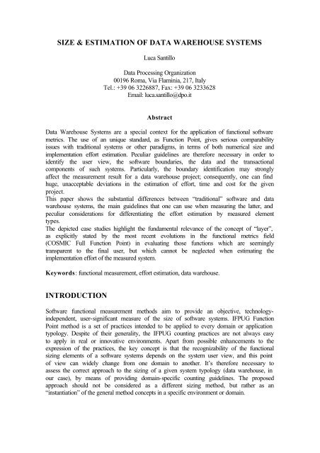
SIZE & ESTIMATION OF DATA WAREHOUSE SYSTEMS<br />
Luca Santillo<br />
Data Processing Organization<br />
00196 Roma, Via Flaminia, 217, Italy<br />
Tel.: +39 06 3226887, Fax: +39 06 3233628<br />
Email: luca.santillo@dpo.it<br />
Abstract<br />
Data Warehouse Systems are a special context for the application <strong>of</strong> functional s<strong>of</strong>tware<br />
metrics. The use <strong>of</strong> an unique standard, as Function Point, gives serious comparability<br />
issues with traditional <strong>systems</strong> or other paradigms, in terms <strong>of</strong> both numerical <strong>size</strong> and<br />
implementation effort <strong>estimation</strong>. Peculiar guidelines are therefore necessary in order to<br />
identify the user view, the s<strong>of</strong>tware boundaries, the <strong>data</strong> and the transactional<br />
components <strong>of</strong> such <strong>systems</strong>. Particularly, the boundary identification may strongly<br />
affect the measurement result for a <strong>data</strong> <strong>warehouse</strong> project; consequently, one can find<br />
huge, unacceptable deviations in the <strong>estimation</strong> <strong>of</strong> effort, time and cost for the given<br />
project.<br />
This paper shows the substantial differences between “traditional” s<strong>of</strong>tware and <strong>data</strong><br />
<strong>warehouse</strong> <strong>systems</strong>, the main guidelines that one can use when measuring the latter, and<br />
peculiar considerations for differentiating the effort <strong>estimation</strong> by measured element<br />
types.<br />
The depicted case studies highlight the fundamental relevance <strong>of</strong> the concept <strong>of</strong> “layer”,<br />
as explicitly stated by the most recent evolutions in the functional metrics field<br />
(COSMIC Full Function Point) in evaluating those functions which are seemingly<br />
transparent to the final user, but which cannot be neglected when estimating the<br />
implementation effort <strong>of</strong> the measured system.<br />
Keywords: functional measurement, effort <strong>estimation</strong>, <strong>data</strong> <strong>warehouse</strong>.<br />
INTRODUCTION<br />
S<strong>of</strong>tware functional measurement methods aim to provide an objective, technologyindependent,<br />
user-significant measure <strong>of</strong> the <strong>size</strong> <strong>of</strong> s<strong>of</strong>tware <strong>systems</strong>. IFPUG Function<br />
Point method is a set <strong>of</strong> practices intended to be applied to every domain or application<br />
typology. Despite <strong>of</strong> their generality, the IFPUG counting practices are not always easy<br />
to apply in real or innovative environments. Apart from possible enhancements to the<br />
expression <strong>of</strong> the practices, the key concept is that the recognizability <strong>of</strong> the functional<br />
sizing elements <strong>of</strong> a s<strong>of</strong>tware <strong>systems</strong> depends on the system user view, and this point<br />
<strong>of</strong> view can widely change from one domain to another. It’s therefore necessary to<br />
assess the correct approach to the sizing <strong>of</strong> a given system typology (<strong>data</strong> <strong>warehouse</strong>, in<br />
our case), by means <strong>of</strong> providing domain-specific counting guidelines. The proposed<br />
approach should not be considered as a different sizing method, but rather as an<br />
“instantiation” <strong>of</strong> the general method concepts in a specific environment or domain.
On the other hand, if we use a specific measurement approach for the given domain, we<br />
have to face the fact that effort <strong>estimation</strong> (<strong>of</strong> development or enhancement activities)<br />
from this measurement cannot be obtained from general models (unless we accept the<br />
strong risk <strong>of</strong> large <strong>estimation</strong> errors). Therefore, an “instantiation” <strong>of</strong> a generic effort<br />
model is to be used.<br />
DATA WAREHOUSE DEFINITIONS<br />
Data Warehouse System<br />
A <strong>data</strong> <strong>warehouse</strong> contains cleansed and organized <strong>data</strong> that allows decision makers to<br />
make business decisions based on facts, not on intuition; it includes a repository <strong>of</strong><br />
information that is built using <strong>data</strong> from the far-flung, and <strong>of</strong>ten departmentally isolated,<br />
<strong>systems</strong> <strong>of</strong> enterprise-wide computing (operational <strong>systems</strong>, or “<strong>data</strong> sources”). Creating<br />
<strong>data</strong> to be analysed requires that the <strong>data</strong> be subject-oriented, integrated, time<br />
referenced and non-volatile. Making sure that the <strong>data</strong> can be accessed quickly and can<br />
meet the ad hoc queries that users need requires that the <strong>data</strong> be organized in a new<br />
<strong>data</strong>base design, the star (schema) or multidimensional <strong>data</strong> model. See Tab. 1 for an<br />
overview <strong>of</strong> peculiar aspects <strong>of</strong> <strong>data</strong> <strong>warehouse</strong> <strong>systems</strong>, versus operational<br />
(transactional) <strong>systems</strong>.<br />
Transaction Processing<br />
Data Warehouse<br />
Purpose Run day-to-day operations Information retrieval and analysis<br />
Structure<br />
RDBMS optimised for Transaction<br />
Processing<br />
RDBMS optimised for Query<br />
Processing<br />
Data Model Normalised Multi-dimensional<br />
Access SQL SQL, plus Advanced Analytical<br />
tools.<br />
Type <strong>of</strong> Data Data that runs the business Data to analyse the business<br />
Nature <strong>of</strong> Data Detailed Summarized & Detailed<br />
Data Indexes Few Many<br />
Data Joins Many Some<br />
Duplicated Data Normalized DBMS Denormalised DBMS<br />
Derived Data &<br />
Aggregates<br />
Rare<br />
Common<br />
Table 1. Data Warehouse <strong>systems</strong> versus transactional <strong>systems</strong>.<br />
Enterprise Data Warehouse (EDW)<br />
An EDW contains detailed (and possibly summarized) <strong>data</strong> captured from one or more<br />
operational <strong>systems</strong>, cleaned, transformed, integrated and loaded into a separate subjectoriented<br />
<strong>data</strong>base. As <strong>data</strong> flows from an operational system into an EDW, it does not<br />
replace existing <strong>data</strong> in the EDW, but is instead accumulated to show a historical record<br />
<strong>of</strong> business operations over a period <strong>of</strong> time that may range from a few months to many<br />
years. The historical nature <strong>of</strong> the <strong>data</strong> in an EDW supports detailed analysis <strong>of</strong> business<br />
trends, and this style <strong>of</strong> <strong>warehouse</strong> is used for short- and long-term business planning<br />
and decision making covering multiple business units.<br />
Data Mart (DM)<br />
A DM is a subset <strong>of</strong> corporate <strong>data</strong> that is <strong>of</strong> value to a specific business unit,<br />
department, or set <strong>of</strong> users. This subset consists <strong>of</strong> historical, summarized, and possibly<br />
detailed <strong>data</strong> captured from operational <strong>systems</strong> (independent <strong>data</strong> marts) , or from an
EDW (dependent <strong>data</strong> marts). Since two or more <strong>data</strong> marts can use the same <strong>data</strong><br />
sources, an EDW can feed both sets <strong>of</strong> <strong>data</strong> marts and information queries, thereby<br />
reducing redundant work.<br />
Data Access Tools (OLAP, On-line Analytical Processing)<br />
OLAP is the technology that enables users to access the <strong>data</strong> “multidimensionally” in a<br />
fast, interactive, easy-to-use manner and performs advanced metric computations such<br />
as comparison, percentage variations, and ranking. The main difference between OLAP<br />
and other generic query and reporting tools is that OLAP allows users to look at the <strong>data</strong><br />
in terms <strong>of</strong> many dimensions.<br />
Meta<strong>data</strong><br />
Simply stated, meta<strong>data</strong> is <strong>data</strong> about <strong>data</strong>. Meta<strong>data</strong> keeps track <strong>of</strong> what is where in the<br />
<strong>data</strong> <strong>warehouse</strong>.<br />
Extraction, Transformation, & Loading (ETL)<br />
These are the typical phases required to create and update a <strong>data</strong> <strong>warehouse</strong> DB:<br />
• In the Extraction phase, operational <strong>data</strong> are moved into the EDW (or<br />
independent DM). The operational <strong>data</strong> can be in form <strong>of</strong> records in the tables <strong>of</strong><br />
a RDBMS or flat files where each field is separated by a delimiter.<br />
• Transformation phase changes the structure <strong>of</strong> <strong>data</strong> storage. The transformation<br />
process is carried out after designing the <strong>data</strong>mart schema. It is a process that<br />
ensures that <strong>data</strong> is moved into the <strong>data</strong>mart, it changes the structure <strong>of</strong> <strong>data</strong><br />
suitable for transaction processing to a structure that is most suitable for DSS<br />
analysis, providing a cleaning <strong>of</strong> the <strong>data</strong> when necessary, as defined from the<br />
<strong>data</strong> <strong>warehouse</strong> manager.<br />
• Loading phase represents an iterative process. The <strong>data</strong> <strong>warehouse</strong> has to be<br />
populated continually and incrementally to reflect the changes in the operational<br />
system(s).<br />
Dimensions<br />
A dimension is a structure that categorizes <strong>data</strong> in order to enable end users to answer<br />
business questions. Commonly used dimensions are Customer, Product, and Time. The<br />
<strong>data</strong> in the structure <strong>of</strong> a <strong>data</strong> <strong>warehouse</strong> system has two important components:<br />
dimensions and facts. The dimensions are products, locations (stores), promotions, and<br />
time, and similar attributes. The facts are sales (units sold or rented), pr<strong>of</strong>its, and similar<br />
measures. A typical dimensional cube is shown in Fig. 1.<br />
Figure 1. Sample Dimensional Cube.
Star Schema<br />
Star Schema is a <strong>data</strong> analysis model analogue to a (multi)dimensional cube view. The<br />
center <strong>of</strong> the star is the fact (or measure) table, while the others are dimensional tables.<br />
Fig. 2 shows an example <strong>of</strong> star schema.<br />
Figure 2. Example <strong>of</strong> Star Schema.<br />
Specifically, dimension values are usually organized into hierarchies. Going up a level<br />
in the hierarchy is called rolling up the <strong>data</strong> and going down a level in the hierarchy is<br />
called drilling down the <strong>data</strong>. For example, within the time dimension, months roll up to<br />
quarters, quarters roll up to years, and years roll up to all years, while within the<br />
location dimension, stores roll up to cities, cities roll up to states, states roll up to<br />
regions, regions roll up to countries, and countries roll up to all countries. Data analysis<br />
typically starts at higher levels in the dimensional hierarchy and gradually drills down if<br />
the situation warrants such analysis.<br />
FUNCTIONAL MEASUREMENT DEFINITIONS<br />
Functional Size<br />
The <strong>size</strong> <strong>of</strong> a (s<strong>of</strong>tware) system as viewed from a logical, non-technical point <strong>of</strong> view. It<br />
is more significant to the user than physical or technical <strong>size</strong>, as for example Lines <strong>of</strong><br />
Code. This <strong>size</strong> should be shared between users and developers <strong>of</strong> the given system.<br />
IFPUG Function Point<br />
IFPUG Function Point measure is obtained by summing up the <strong>data</strong> and the<br />
transactional functions, classified as Internal Logical Files, External Interface Files, and<br />
External Inputs, Outputs, or Inquiries, with respect to the application boundary, which<br />
divides the measured system from the user domain(or interfaced <strong>systems</strong>). See Tab. 2<br />
for an overview <strong>of</strong> the numerical weights (here “complexity” depends depends on<br />
logical structure <strong>of</strong> each element, in terms <strong>of</strong> quantities <strong>of</strong> logical attributes and<br />
referenced files contained or used by files or transactions).<br />
Low Complexity Average Complexity High Complexity<br />
ILF 7 10 15<br />
EIF 5 7 10<br />
EI 3 4 6<br />
EO 4 5 7<br />
EQ 3 4 6<br />
Table 2. Function Point elements’ weights.
COSMIC Full Function Point<br />
COSMIC Full Function Point has been proposed as a superset <strong>of</strong> functional metrics,<br />
which provides wider applicability than the IFPUG method. Its key concepts are the<br />
possibility <strong>of</strong> viewing the measured system under different linked layers (different<br />
levels <strong>of</strong> conceptual abstraction <strong>of</strong> the system functions) and the possibility to extend its<br />
practices with “local extensions”.<br />
FUNCTIONAL SIZE OF DATAWAREHOUSE SYSTEMS<br />
IFPUG <strong>of</strong>ficial documentation doesn’t provide specific examples for counting <strong>data</strong><br />
<strong>warehouse</strong> <strong>systems</strong>; on the other hand, this kind <strong>of</strong> system is growing in importance and<br />
diffusion among private and public companies. We therefore need some guidelines,<br />
especially if we consider the special user view and consequent specific <strong>data</strong> models for<br />
this system type.<br />
A generic <strong>data</strong> <strong>warehouse</strong> system can be viewed as made <strong>of</strong> three segments: Data<br />
Assembling (see ETL above), System Administration (see also Meta<strong>data</strong> above), and<br />
Data Access (see OLAP above).<br />
Type <strong>of</strong> Count<br />
Determining the type <strong>of</strong> count (Development project, Enhancement Project, or<br />
Application) is usually easy, and doesn’t require specific guidelines for <strong>data</strong> <strong>warehouse</strong><br />
<strong>systems</strong>. We just remind that adding or changing functionality <strong>of</strong> a given system could<br />
be considered as one or more (development and enhancement) projects, depending on<br />
which system boundaries are firstly identified.<br />
User View<br />
Many figures contributes to constitute a <strong>data</strong> <strong>warehouse</strong> user:<br />
• ETL procedures administrator,<br />
• DB administrator,<br />
• OLAP (or other access means) administrator,<br />
• final user (who have access to the <strong>data</strong> <strong>warehouse</strong> information),<br />
• any system providing or receiving <strong>data</strong> to or from the <strong>data</strong> <strong>warehouse</strong> system (for<br />
example, operational <strong>systems</strong> which automatically send <strong>data</strong> to the ETL<br />
procedures).<br />
Application Boundary<br />
When considering the separation between <strong>systems</strong> in the <strong>data</strong> <strong>warehouse</strong> domain, the<br />
application boundaries should:<br />
• be coherent with the organizational structure (e.g. each department has its own DM)<br />
• reflect the project management autonomy <strong>of</strong> the EDW with respect to any DM,<br />
• reflect the project management autonomy <strong>of</strong> each DM with respect to any other.<br />
The following picture (Fig. 3) shows the proposed approach to the boundary question in<br />
a <strong>data</strong> <strong>warehouse</strong> context. Note that the shown boundaries are orthogonal to the<br />
segmentation by phase <strong>of</strong> the <strong>data</strong> <strong>warehouse</strong> system (ETL, Administration, Access).
Administration<br />
(EDW)<br />
Metadat<br />
Administration<br />
(DM)<br />
Metadat<br />
ETL EDW<br />
DB (EDW)<br />
ETL DM<br />
DM (dependent)<br />
Metadati<br />
ETL DM<br />
Operational<br />
Data<br />
DM<br />
ETL (EDW) ETL (DM) Data Access<br />
Figure 3. Boundary scheme for EDW, dependent DM, and independent DM.<br />
Comments on boundaries<br />
Note that, as stated also by the IFPUG Counting Practices Manual, some <strong>systems</strong> could<br />
share some functionality, and each <strong>of</strong> them should count those functions. For example,<br />
2 or more (dependent / independent) DMs’ can make use <strong>of</strong> the same external source<br />
files (EDW / operational) in order to load their own <strong>data</strong>. While counting these shared<br />
functions for each system which uses them, we should not ignore some reuse<br />
consideration, when deriving the effort <strong>estimation</strong> for each system development or<br />
enhancement project.<br />
Boundary re-definition should be performed only in special cases, as the merge <strong>of</strong> 2<br />
DMs’ into one, or the split <strong>of</strong> 1 DM into more than one system. In doing such a redefinition,<br />
we have to mark some functions as deleted without effort (in the merge<br />
case), or as duplicated without effort.<br />
Data Functions<br />
Operational source <strong>data</strong><br />
These are EIFs’ for the EDW or the independent DM which use them in the ETL<br />
segment. While the separation into distinct logical files is performed from the point <strong>of</strong><br />
view <strong>of</strong> the operational system which provides and contains them as its own ILFs’, their<br />
content, in terms <strong>of</strong> Data Element Types, and Record Element Types, should be counted<br />
from the point <strong>of</strong> view <strong>of</strong> the target system. Note that simple physical duplicates on<br />
different areas are usually not counted as different logical files.<br />
A special case <strong>of</strong> the ETL procedure is when the operational system provides by its own<br />
procedures the information to the EDW (or independent DM); in this case, no EIF is<br />
counted for the latter, since we have External Outputs sending out <strong>of</strong> the source system<br />
the information required, and not the target system reading and collecting the <strong>data</strong>.
Data <strong>warehouse</strong> internal <strong>data</strong> - Star schema <strong>data</strong> model<br />
While counters are provided with sufficient guidelines and example for entityrelationship<br />
<strong>data</strong> models, we have to face the case <strong>of</strong> star schema <strong>data</strong> models, which<br />
correspond to the multidimensional cube views.<br />
Since the fact table is not significant to the <strong>data</strong> <strong>warehouse</strong> user, without its dimensional<br />
tables, and vice versa, we suggest the strong guideline that each “logical” star is an ILF<br />
for the EDW or DM being counted. Each (fact and dimensional) table is a Record<br />
Element Type for such a logical file. IN analogy with this, each “logical” cube is an<br />
ILF, with N+1 RET, where N is the number <strong>of</strong> its dimensions (the axes <strong>of</strong> the cube).<br />
In case <strong>of</strong> the so-called snow-flake schema, where the hierarchical dimensions are<br />
exploded into their levels (e.g. month – quarter - year), the second order tables do not<br />
represent other RETs’, since the counted RET is for the whole dimension (“time” in the<br />
cited example).<br />
The DETs’ <strong>of</strong> each hierarchy are only two, dimension level and value (e.g. “time level”,<br />
which can be “month”, “quarter”, “year”, and “time value”, which can be “January”,<br />
“February”, …, “I”, “II”, …, “1999”, “2000”, …, and so on).<br />
Other attributes in the tables, apart from those who implement a hierarchy , are counted<br />
as additional DETs’ for the logical file. A special case <strong>of</strong> <strong>data</strong> <strong>warehouse</strong> <strong>systems</strong><br />
attributes is that <strong>of</strong> pre-derived <strong>data</strong>, or <strong>data</strong> which are firstly derived in the ETL phases,<br />
then recorded in the file, and finally accessed by the final user, in order to provide the<br />
maximum performance. A logical analysis should be carried in order to distinguish the<br />
case when the (final) user recognises these <strong>data</strong> as contained in the files, and then only<br />
retrieved by inquiries, from the case when the user is not aware <strong>of</strong> such a physical<br />
processing, and considers the <strong>data</strong> as derived online by the required output process.<br />
Meta<strong>data</strong><br />
Technical meta<strong>data</strong>, as update frequency, system versioning, physical-logical files<br />
mapping, are not identifiable as logical files. Since the <strong>data</strong> <strong>warehouse</strong> administrator is<br />
one <strong>of</strong> the figures which constitute the general system user, some meta<strong>data</strong> can be<br />
recognized and counted as logical files; example are:<br />
• User pr<strong>of</strong>iles file<br />
• Access Privileges file<br />
• Data processing rules file<br />
• Use Statistics file<br />
Business meta<strong>data</strong> are good candidates for being counted as logical files; examples are:<br />
• Data dictionary(what is the meaning <strong>of</strong> an attribute)<br />
• Data on historical aspects (when a value for an attribute was provided)<br />
• Data on the <strong>data</strong> owner (who provided a value for an attribute)<br />
Transactional Functions
ETL: we suggest the strong guideline that the overall procedure <strong>of</strong> reading external<br />
source files, cleaning and transforming their contents, reading eventually meta<strong>data</strong>, and<br />
loading the derived information in the target system is a unique process from the <strong>data</strong><br />
<strong>warehouse</strong> user point <strong>of</strong> view; therefore we have only one EI for each target identified<br />
ILF. DETs’ <strong>of</strong> such an EI should be all the attributes which enters the boundary <strong>of</strong><br />
system being counted, plus the eventual output attributes or <strong>data</strong>, such as messages to<br />
the user for error or confirmation.<br />
Administration: The administration segment contains traditional processes, such as the<br />
management transactions for creating, updating, deleting, and viewing meta<strong>data</strong>.<br />
Access: The main functions <strong>of</strong> the access segment are those who let the user consult<br />
information from the <strong>data</strong> <strong>warehouse</strong>; such processes are counted as EOs’ or EQs’,<br />
depending on the presence <strong>of</strong> derived <strong>data</strong>. Therefore, we have at least 1 process<br />
(usually EO) for each identified “logical star” <strong>of</strong> the <strong>data</strong> <strong>warehouse</strong> DB. Note that<br />
drilling down o rolling up the same star is equivalent to retrieving the same <strong>data</strong>, just<br />
using different “levels” in the dimensional hierarchies – which are all DETs’ <strong>of</strong> the<br />
same star – so different levels <strong>of</strong> the view are counted only once, as they are the same<br />
logical output.<br />
The drill down trigger itself is usually provided by common OLAP tools as a listbox on<br />
every “drillable” attribute. Such mechanism is counted as a low complexity EQ (for<br />
each distinct attribute <strong>of</strong> each distinct star), while the productivity coefficient for such a<br />
process will strongly reduce its impact.<br />
Function Taxonomy Classes<br />
In order to support the effort <strong>estimation</strong>, the <strong>data</strong> and transactional functions should be<br />
labelled depending on their role in the <strong>data</strong> <strong>warehouse</strong> system being measured. The<br />
classes are: ETL (Extraction, Transformation & Loading), ADM (Administration), ACC<br />
(Access). Tab. 3 provides examples <strong>of</strong> such a classification.<br />
Type Where Examples<br />
ILF ETL EDW, DM • EDW DB logical files<br />
• Independent DM DB logical files<br />
• Dependent DM DB logical files, when logically distinct from<br />
the EDW DB logical files<br />
ILF ADM EDW, DM Meta<strong>data</strong>, significant LOG files, statistics<br />
EIF ETL EDW, DM Operational DB logical files<br />
EIF EDW Dependent DM EDW’s ILFs’, when accessed by ETL or Access procedure<br />
EIF ADM EDW, DM • Significant support files<br />
• Externally maintained meta<strong>data</strong><br />
EI ETL EDW, DM 1 EI for each identified ILF ETL<br />
EI ADM EDW, DM Create, update, delete meta<strong>data</strong><br />
EO ADM EDW View meta<strong>data</strong> (with derived <strong>data</strong>)<br />
EQ ADM EDW View meta<strong>data</strong> (without derived <strong>data</strong>)<br />
EO ACC DM 1 EO for each identified ILF ETL<br />
EQ ACC DM 1 EQ for each identified ILF ETL which has no corresponding<br />
EO ACC , i.e. view without any derived <strong>data</strong><br />
EQ LISTBOX DM Drill-down triggers, any other List Boxes<br />
Table 3. Function Types Taxonomy.
Value Adjustment Factor (VAF)<br />
At the present moment, a specific ISO Working Group is examining the candidates for a<br />
standard s<strong>of</strong>tware functional measurement definition; one preliminary result is that the<br />
14 General System Characteristics, which constitute the VAF, should not be used;<br />
therefore, we neglect VAF, or, that is equivalent, we consider its value equal to 1 in any<br />
counting case.<br />
Final Function Point Formulas<br />
Standard formulas are used without specific recommendation. We only recall the use <strong>of</strong><br />
the proposed taxonomy; that means that, besides total <strong>of</strong> FP, we have to provide the<br />
complete list <strong>of</strong> different functions, depending on their classes. Since we always assume<br />
a VAF = 1 for <strong>data</strong> <strong>warehouse</strong> <strong>systems</strong>, the final count formulas are slightly simplified.<br />
EFFORT ESTIMATION FOR DATAWAREHOUSE SYSTEMS<br />
Data <strong>warehouse</strong> <strong>systems</strong> productivity factors<br />
The main peculiar productivity aspects <strong>of</strong> <strong>data</strong> <strong>warehouse</strong> <strong>systems</strong> are:<br />
• Many <strong>data</strong> and transactional functions are cut (flatten) because <strong>of</strong> the limit <strong>of</strong><br />
“high complexity”<strong>of</strong> the IFPUG model;<br />
• Internal and external reuse can be very significant;<br />
• Data <strong>warehouse</strong> and OLAP tools and technology positively impact the<br />
implementation productivity, while the analysis phase can be very consuming<br />
• Some segments (as Access) are more impacted by the use <strong>of</strong> tools.<br />
All these factors lead us to consider an innovative structured approach to the utilization<br />
<strong>of</strong> Function Point measure in the s<strong>of</strong>tware effort <strong>estimation</strong> process, when applied to<br />
<strong>data</strong> warehopuse <strong>systems</strong>. Instead <strong>of</strong> putting the mere total number <strong>of</strong> FP for a project in<br />
a benchmarking regression equation, we found by empirical and heuristical research<br />
some steps which provides an “adjusted” number, that can be seen as “FP-equivalent”<br />
for effort <strong>estimation</strong> purpose. Of course, we should keep the original counted FP as the<br />
<strong>size</strong> <strong>of</strong> the system in terms <strong>of</strong> the user view, while this “FP-equivalent” is a more<br />
realistic number to use in a s<strong>of</strong>tware effort <strong>estimation</strong> model. The coefficients proposed<br />
in the following are to be multiplied with the original FP number <strong>of</strong> the corresponding<br />
counted function. Only cases different from unitary (neutral) adjustment are shown.<br />
1. Adjustment by intervention class (only specific classes are shown)<br />
DEV EDW ENH EDW DEV DM ENH DM<br />
Class Coefficient Coefficient Coefficient Coefficient<br />
ILF ETL 1 1<br />
⎛ RET − 4 ⎞ ⎛ RET − 4 ⎞<br />
⎜1 + ⎟ ⎜1<br />
+ ⎟<br />
⎝ 4 ⎠ ⎝ 4 ⎠<br />
EI ETL<br />
EO ACC<br />
EQ ACC<br />
⎛ FTR − 3 ⎞ ⎛ FTR − 3 ⎞ ⎛ FTR − 4 ⎞ ⎛ FTR − 4 ⎞<br />
⎜2 + ⎟ ⎜2 + ⎟ ⎜1 + ⎟ ⎜1<br />
+ ⎟<br />
⎝ 3 ⎠ ⎝ 3 ⎠ ⎝ 3 ⎠ ⎝ 3 ⎠<br />
⎛ FTR − 4 ⎞ ⎛ FTR − 4 ⎞<br />
⎜1 + ⎟ ⎜1 + ⎟ 1 1<br />
⎝ 4 ⎠ ⎝ 4 ⎠<br />
⎛ FTR − 3 ⎞ ⎛ FTR − 3 ⎞<br />
⎜1 + ⎟ ⎜1 + ⎟ 1 1<br />
⎝ 3 ⎠ ⎝ 3 ⎠<br />
Table 4. Adjustment coefficients by intervention class.
2. Adjustment by reuse (NESMA-like model)<br />
2a. Development (both EDW & DM)<br />
Consider each function class in the given count (e.g. all the ILF ETL , then all EIF ETL , and<br />
so on). For each distinct function class:<br />
a) Assign a reuse coefficient <strong>of</strong> 0.50 to each function (except the 1 st ) <strong>of</strong> the set <strong>of</strong><br />
functions which share:<br />
• 50% or more DETs’, and 50% or more RETs’ or FTRs’.<br />
b) Assign a reuse coefficient <strong>of</strong> 0.75 to each function (except the 1 st ) <strong>of</strong> the residue<br />
set <strong>of</strong> functions which share:<br />
• 50% or more DETs’, but less than 50% RETs’ or FTRs’;<br />
• less than 50% DETs’, but 50% or more RETs’ or FTRs’.<br />
c) Assign a reuse coefficient <strong>of</strong> 1.00 (neutral) to the residue.<br />
The “1 st function” means the function in the given class with highest functional<br />
complexity, highest number <strong>of</strong> DETs’, highest number <strong>of</strong> RETs’ or FTRs’. The percent<br />
values <strong>of</strong> DETs’, RETs’, and FTRs’, are determined with respect to this “1 st function”.<br />
In the special case <strong>of</strong> CRUD transactions sets in Administration segment, i.e. Create,<br />
Read, Update, and Delete <strong>of</strong> generic file type, assign a uniform 0.5 adjustment to each<br />
transaction in the unique identified CRUD.<br />
2b. Enhancement (both EDW & DM)<br />
Added Functions<br />
Act as for Development.<br />
Internally Changed Functions (i.e. added, changed, deleted DETs’, RETs’, or FTRs’)<br />
DET%<br />
Reuse ENH<br />
≤ 33% ≤ 67% ≤ 100% > 100%<br />
≤ 33% 0.25 0.50 0.75 1.00<br />
RET%<br />
≤ 67% 0.50 0.75 1.00 1.25<br />
or<br />
≤ 100% 0.75 1.00 1.25 1.50<br />
FTR% > 100% 1.00 1.25 1.50 1.75<br />
Table 5. Reuse coefficients for Internlly Changd Functions.<br />
where the percent values are given by comparing the number <strong>of</strong> DETs’, RETs’, FTRs’<br />
which are added, modified, or deleted, with respect to their pre-enhancement quantities.<br />
Type Changed Functions (i.e. ILF to EIF, EQ to EO, etc.)<br />
Assign an adjustment reuse coefficient <strong>of</strong> 0.4.<br />
Mixed Cases<br />
If a function is changed in both internal elements and type, assign the higher <strong>of</strong> the two<br />
adjustment coefficients from the above. For transactions, note that changes in the user<br />
interface, layout, or fixed labels, without changes in the processing logic, are not<br />
considered.
Deleted Functions<br />
Assign an adjustment reuse coefficient <strong>of</strong> 0.4.<br />
3. Adjustment by technology (only applied to DM projects, Access segment)<br />
DEV DM ENH DM<br />
Class Coefficient Coefficient<br />
EO ACC 0.5 0.5<br />
EQ ACC 0.5 0.5<br />
EQ LISTBOX 0.1 0.1<br />
Table 6. DW technology adjustments.<br />
Effort Estimation<br />
After we obtain the “FP-equivalent” frm the previous adjustment, we can put its value<br />
in a benchmarking regression equation, as the following, which has been obtained (by<br />
filtering on several sample attributes) from the ISBSG Benhmark:<br />
Avg.Eff = 13.92 x FP-equivalent - 371.15<br />
Note that this equation is just an example; more precise <strong>estimation</strong>s can be obtained<br />
only by creating a “local benchmark” for the given company, project team, or<br />
department. However, one further step is still to be made: specific productivity<br />
adjustment <strong>of</strong> the average effort estimate.<br />
Specific productivity adjustment<br />
This last step is carrie dout by means <strong>of</strong> the well-known COCOMO II model; we recall<br />
that only some factors <strong>of</strong> the original COCOMO II model are to be used, since, for<br />
example, the REUSE factor is already explicitly considered in the previous steps, when<br />
calculating the FP-equivalent.<br />
The final effort <strong>estimation</strong> is therefore:<br />
Effort = Effort ⋅<br />
where:<br />
• Effort is the Average Effort from the previous step, based on ISBSG or<br />
equivalent benchmark.<br />
• CD i is the coefficient <strong>of</strong> the ith COCOMO II Cost Driver.<br />
N<br />
∏<br />
i=<br />
1<br />
CD i<br />
The Cost Driver considered in the actual research are:<br />
• RELY (Required s<strong>of</strong>tware reliability)<br />
• CPLX (Product complexity)<br />
• DOCU (Documentation match to life-cycle needs)<br />
• PVOL (Platform volatility)<br />
• ACAP (Analyst capabilities)<br />
• PCAP (Programmer capabilities)<br />
• AEXP (Applications experience)<br />
• PEXP (Platform experience)
Readers should refer to the original COCOMO II documentation for exact values <strong>of</strong> the<br />
levels <strong>of</strong> these drivers.<br />
COMMENTS & CONCLUSIONS<br />
Serious testing <strong>of</strong> the proposed approach is being carried out at the moment. Further<br />
developments will surely come from the adoption <strong>of</strong> the COSMIC Full Function Point<br />
“layer” concept, which will is able to take into account the impact <strong>of</strong> some specific<br />
“segments” <strong>of</strong> <strong>data</strong> <strong>warehouse</strong> <strong>systems</strong>, as for example a detailed model <strong>of</strong> the ETL<br />
(Extraction, Transformation & Loading) phases, in order to improve the effort<br />
<strong>estimation</strong> precision. Moreover, research pointed out the inadequacy <strong>of</strong> cut limits in the<br />
complexity levels <strong>of</strong> IFPUG Function Point method, as already shown by the ISBSG<br />
research: some rangs in the complexity matrices should be revised or extended. Note<br />
that in COSMIC Full Function Point method, there no such artificial cut-<strong>of</strong>f.<br />
Another issue that is to be faced is the creation <strong>of</strong> specific benchmark for <strong>data</strong><br />
<strong>warehouse</strong> domain and technology, since this typology is going to play an relevant role<br />
in the future <strong>of</strong> public and private companies, which have to manage more and more<br />
information in less and less time than ever.<br />
REFERENCES<br />
• Baralis E., “Data Mining”, Politecnico di Torino, 1999<br />
• COCOMO II Model Definition Manual rel. 1.4, University <strong>of</strong> Southern<br />
California, 1997<br />
• COSMIC Full Function Point Measurement Manual, Version 2.0, Serge<br />
Oligny, 1999<br />
• Hennie Huijgens, “Estimating Cost <strong>of</strong> S<strong>of</strong>tware Maintenance: a Real Case<br />
Example”, NESMA , 2000<br />
• Dyché J., “e-Data: Turning Data into Information with Data Warehousing”,<br />
Addison-Wesley, 2000<br />
• IFPUG Function Point Counting Practices Manual, Release 4.1, IFPUG,<br />
1999<br />
• ISBSG Benchmark, Release 6, ISBSG, 2000<br />
• Torlone R., “Data Warehousing”, Dipartimento di Informatica e Automazione,<br />
Università di Roma Tre, 1999