Rotation Points From Motion Capture Data Using a ... - CiteSeerX

Rotation Points From
Motion Capture Data Using a Closed Form Solution
by
JONATHAN KIPLING KNIGHT
M.A. Applied Mathematics, Cal. State Fullerton, 1995
B.S. Physics, Cal Poly, San Luis Obispo, 1987
A thesis submitted to the Graduate Faculty of the
University of Colorado at Colorado Springs
in partial fulfillment of the requirements for the degree of
Doctor of Philosophy
Department of Computer Science
2008

ii
Acknowledgements
First and foremost I would like to acknowledge my wife Kiki for her patience during
this research. I would also like to thank Gene Johnson for his support during the ups
and downs of my life during this major event in my life. He kept telling me to continue.
I would also like to thank my advisor Dr. Semwal for allowing me the freedom and guidance
to pursue the ideas laid down in this paper.
© Copyright by Jonathan Kipling Knight 2007-2008, All Rights Reserved

iii
This thesis for the Philosophical Doctor degree by
Jonathan Kipling Knight
has been approved for the
Department of Computer Science
by
______________________________
Sudhanshu Kumar Semwal, Chair
______________________________
Robert Carlson
______________________________
C. Edward Chow
______________________________
Jugal Kalita
______________________________
Charles M. Shub
________________________
Date

iv
Knight, Jonathan Kipling (Ph.D., Computer Science)
Rotation Points from Motion Capture Data Using a Closed Form Solution
Thesis directed by Professor Sudhanshu Kumar Semwal
Four new closed-form methods are present to find rotation points of a skeleton
from motion capture data. A generic skeleton can be directly extracted from noisy data
with no previous knowledge of skeleton measurements. The new methods are ten times
faster than the next fastest and a hundred times faster than the most widely accepted
method. Two phases are used to produce an accurate skeleton of the captured data. The
first phase, fitting the skeleton, is robust even with noisy motion capture data. The formulae
use an asymptotically unbiased version of the Generalized Delogne-Kása (GDKE)
Hyperspherical Estimation (first estimator: UGDK). The second estimator takes advantage
of multiple markers located at different distances from the rotation point (MGDK)
thereby increasing accuracy. The third estimator removes singularities to allow for cylindrical
joint motion (SGDK). The fourth estimator incrementally improves an answer
and has advantages of constant memory requirements suitable for firmware applications
(IGDK). The UGDK produces the answer faster than any previous algorithm and with
the same efficiency with respect to the Cramér-Rao Lower Bound for fitting spheres and
circles. The UGDK method significantly reduces the amount of work needed for calculating
rotation points by only requiring 26N flops for each joint. The next fastest method,
Linear Least-Squares requires 236N flops. In-depth statistical analysis shows the UGDK
method converges to the actual rotation point with an error of O(σ/√N) improving on the
GDKE’s biased answer of O(σ). The second phase is a real-time algorithm to draw the

v
skeleton at each time frame with as little as one point on a segment. This speedy method,
on the order of the number of segments, aids the realism of motion data animation by allowing
for the subtle nuances of each time frame to be displayed. Flexibility of motion is
displayed in detail as the figure follows the captured motion more closely. With the reduced
time complexity, multiple figures, even crowds can be animated. In addition, calculations
can be reused for the same actor and marker-set allowing different data sets to
be blended. The main contributions in this dissertation are the new unbiased center formulae;
the full statistical analysis of this new formula; and the analysis of when the best
measurement conditions are to initiate the formula. The dissertation further establishes
the application of these new formulae to motion capture to produce a real-time method of
drawing skeletons of arbitrary articulated figures.

vi
CONTENTS
PREFACE
xiii
Chapter 1 INTRODUCTION 1
1.1 Articulated Figure Animation 4
1.2 Motion Capture Systems 7
1.3 Symbols and Conventions 9
Chapter 2 STATEMENT OF THE PROBLEM 11
2.1 Why are skeleton calculations required 11
2.2 Problems encountered 12
2.2.1 Inaccuracies 12
2.2.2 Non-standard Files 13
2.2.3 Missing Data 13
Chapter 3 SURVEY 14
3.1 Skeleton Extraction 14
3.2 Sphere Estimates 14
3.3 Inverse Kinematics 17
3.4 Kinetics 18
Chapter 4 PREVIOUS SOLUTIONS 19
4.1 Spherical Curve-fitting Approaches 19
4.1.1 Monte-Carlo Experiment 19
4.1.2 Cramér-Rao Lower Bound 23

vii
4.1.3 Non-linear Maximum-Likelihood Estimator 34
4.1.4 Linear Least-Squares Solution 37
4.1.5 Generalized Delogne-Kása Estimator 40
4.2 Skeleton Approaches 62
Chapter 5 PROPOSED SOLUTION 64
5.1 Unbiased Generalized Delogne-Kása Estimator 64
5.1.1 Derivation 64
5.1.2 Statistical Properties 66
5.2 Cylindrical Joint Solution 75
5.3 Multiple Marker Solution 76
5.4 Incrementally Improved Solution 78
5.5 Hierarchical Skeleton Solution 81
5.5.1 Arbitrary Figure 81
5.5.2 Predefined Marker Association 86
Chapter 6 RESULTS 90
6.1 Case Study of CMU Data 60-08 90
6.2 Case Study of Eric Camper Data 94
6.3 Comparison 95
6.4 Speed 96
6.5 Conclusion 98
6.6 Important Contributions 99
6.7 Further Research 101

viii
Chapter 7 APPENDIX 102
7.1 Mathematical Proofs 102
7.1.1 Moments of Multivariate Normal 102
7.1.2 Positive-Semidefinite Sample Covariance 110
7.2 Inertial Properties of a Tetrahedron 111
7.3 File Formats 114
7.3.1 Marker Association Format 114
7.3.2 Articulated Tetrahedral Model Format 115
7.3.3 MESH Format 117
7.3.4 PLY Format 121
7.3.5 C3D Format 121
7.4 User’s Guide to Program 121
7.4.1 Menu 122
7.4.2 Options Pane 126
7.4.3 Animation Pane 127
7.4.4 Graphs Pane 129
7.5 Programmer’s Reference 130
7.5.1 Class Diagrams 130
7.6 C++ Implementations 132
7.6.1 Unbiased Generalized Delogne-Kása Method 132
7.6.2 Incrementally Improved Generalized Delogne-Kása 133
7.6.3 Collecting the Raw Data for Rotation Point 134
7.6.4 Rotation Point Calculation of Segment 136
7.6.5 Constants Calculation of Hierarchical Articulated Data 137
7.6.6 Calculation of fixed axes of data 139
7.6.7 Drawing Rotation Points with Constants of Motion 140

ix
Chapter 8 BIBLIOGRAPHY 143
Chapter 9 INDEX 151

x
TABLES
Table 1 Marker Associations 86
Table 2 Table of Means of Rotation Points 90
Table 3 Table of Standard Deviations of Rotation Points 91
Table 4 Comparison of Center Estimators 95
Table 5 Primitives in MESH Format 117
Table 6 Preservation Adjectives in MESH Format 118
Table 7 Optional Adjectives of Primitives in MESH Format 119

xi
FIGURES
Figure 1 Display of Motion-Capture Data
xv
Figure 2 Markers on Actor 2
Figure 3 Human Articulated Shoulder 5
Figure 4 Human Elbow 6
Figure 5 Video Capture Analysis Software (SIMI°MotionCapture 3D) 1 8
Figure 6 Vicon BodyBuilder Software 9
Figure 7 Constrained Measurements on Circle 20
Figure 8 Relative Error Comparison 22
Figure 9 Eigenvectors of CRLB for Circle 28
Figure 10 Eigenvalues of CRLB for Circle 29
Figure 11 Eigenvectors of CRLB for Sphere 32
Figure 12 Eigenvalues of CRLB for Sphere 33
Figure 13 MLE Compared to CRLB 36
Figure 14 MLE Error Versus Sphere Coverage 36
Figure 15 LLS Compared to CRLB 39
Figure 16 GDKE Compared to CRLB 43
Figure 17 GDKE Error Ellipse 48
Figure 18 UGDK Error Ellipse 68
Figure 19 Sample Size Dependency of Deviation 69
Figure 20 One hundred samples comparison of MLE (green), UGDK (red), GDKE (blue) 70
Figure 21 UGDK Compared to CRLB 70
Figure 22 Circle with Constrained Data 72
Figure 23 MGDK example 78
Figure 24 Inverse Power Law for Rotation Point Calculation 94
Figure 25 Eric Camper Skeleton 94
Figure 26 Timing of Algorithms 97
Figure 27 Timing Comparison to GDKE 98

xii
Figure 28 File Menu GUI 123
Figure 29 Options Pane GUI 127
Figure 30 Animation Pane GUI 128
Figure 31 Graphs Pane GUI 129
Figure 32 UML Diagram of Articulated Figure 131

xiii
PREFACE
The research that will be presented in this paper is the culmination of a story. The
five-year journey involves the typical parts of a novel with protagonist, antagonists,
heartaches, and triumphs. The protagonist is, of course, me – the author. The antagonists
in this story were the many hurdles that I stumbled over to finally realize what my actual
goal was for the research. The story of this research is a good example of what it means
for the research topic itself to tell you are going in the wrong direction. Perseverance has
declared a victory in the research only by finally exposing a vital and missing piece of the
puzzle that builds up the topic at hand.
So, what is the topic The research started out five years ago as an idea that current
technology for articulated motion analysis and display was much too slow and unrealistic.
I started the research, albeit naively, by thinking that a combination of physics
and genetic algorithms could infuse a sense of realism and speed into analyzing the motion.
So I sat down and coded up the infrastructure needed to build up this combination.
First, I needed a computer representation of an articulated figure. To keep physics
in the equation, I decided to make each segment of the figure solid. I found that, for
physics related simulations, this is the only way to go since calculations of inertial moments
are fairly simple (cf. Chapter 7.2). A few other authors use this approach for highend
physical simulations but, for the most part, most use triangulated surfaces for their
“solid” figures. It is usually difficult to calculate moments of inertia from only the surface
data. A tetrahedral solid mesh was chosen to simplify building up an arbitrary
shape. With a solid shape, and its mass, the rotational and translational physics are fully
calculable from the Newton-Euler differential equation. As I progressed further in the

xiv
research, I found it increasingly time-intensive to calculate projected motions based on
solving the second-order differential equation on an arbitrary articulated figure.
This suggested that I pursue an alternative approach. So, what if I relied more on
motion-capture data and infuse only a little bit of physics I then looked at reading in
and using raw motion-capture data. Little did I know that motion-capture data was excruciatingly
hard to acquire both on your own and on the Internet. The people and companies
that did any kind of work with capturing motion data were usually quite willing to
sell it. Only a few free examples were found that were of any use. A file reader was built
from scratch for the most popular format since no one had open source code. I struggled
for a year with reading the quirky data format with the small amount of data I found until
a goldmine was found. Carnegie-Melon University Graphics Laboratory had just started
placing a large cache of raw and analyzed motion-capture data on the Internet through a
government grant. I subsequently downloaded gigabytes of raw binary data for a plethora
of motions captured by the students at this lab. One problem solved – gathering data
to analyze.
Now I set about trying to analyze the raw data so that I may use it to better analyze
the underlying articulated motion. Starting with the simplest issue, I started trying to
display the motion on a 3-D scene. As it turns out, the raw data was very inconsistent in
storing which measurement units it was using. Sometimes it was in meters, sometimes it
was in feet, sometimes it was stored in feet and the format said it was meters. Once you
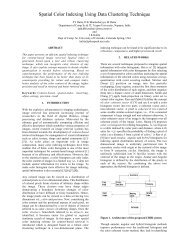
figure out what scale the data is in, you can display the points on the screen.

xv
Figure 1 Display of Motion-Capture Data
Now, all I had was a bunch of squirrelly lines on the screen (cf. Figure 1). Clearly, the
lines had to be associated and grouped. Each line was attached (i.e. correlated) to a particular
segment on the articulated figure. This can be done in one of two ways – autocorrelation
and precognition. I chose the latter since autocorrelation is extremely time intensive.
Precognition may sound like cheating but nine times out of ten, the user will know
ahead of time which bits of data are associated with which segment on the articulated
figure.
What do I have so far I have a bunch of lines that each segment can follow in
time. As data shows marker location at each time frame, each segment has some surface
positions pin-pointed in space. In addition, exact marker location on segments usually
were not known or given. That leaves an unsavory taste in your mouth when the segment
can be placed almost anywhere relative to these points. A systematic approach must be

xvi
thought of that allows the conclusive attachment of the segments to the data. This implies
that the data must contain both relative position and orientation of the segment so
the model can be sized and oriented into position. This satisfies an individual segment,
but not the whole articulated figure. For that I needed the rotation points in between the
segments. What this boils down to is that I needed to draw a stick figure based solely on
the motion-capture data. I could then attach whatever shape model I wanted onto the
stick figure. I did a search for existing methods and found a few examples in the literature
(cf. Chapter 8). The most popular was to perform a least-squares fit and a few still
did non-linear fitting of the data. They all had one thing in common – they all assumed
the marker moved on a sphere around the rotation point of the joint. This means that, to
draw a stick figure, I had to solve for the center of a sphere at every joint. A little research
showed there were only three major algorithms to solve for the center of a sphere
by data points sitting on the sphere. The most popular was the Maximum-Likelihood Estimator
(MLE) that solved the problem in a non-linear fashion. This had the undesirable
effect of being excruciatingly slow and sometimes not producing an answer at all. The
next most popular type was linear least-squares solutions that involve fairly slow (but
faster than MLE) pseudo-inverse matrix solutions. This was the preferred method by
most authors concerned with speed. The third type of solution was a small set of approximations
that were closed-form solutions to the best-fit sphere. These formulae were
unpopular and usually used only in the case to start off a non-linear search for the real
answer. They were unpopular because of biases introduced.
I was unsatisfied with any of these solutions found in the existing literature. They
would get me to the answer, but they were too slow or quirky. I decided to sit back and

xvii
analyze a case study of a particular joint movement. To proceed with analyzing, the raw
(x,y,z) data was loaded into a spreadsheet for the step-by-step analysis to see how the rotation
point could be retrieved from the data. A column of distances from an unknown
point (the rotation point) was made for each data point. Then, thinking about it – what
would happen if the unknown point were truly at the center of rotation Then, the distances
to the data points would all be about the same. What this translates into is that the
standard deviation from the mean of the distances would be minimized. This can be easily
done in Excel with the Solve tool. Thinking about it further, that this is exactly what
the Maximum Likelihood Estimator (MLE) solution is – minimizing the standard deviation
of the distance to the center of rotation. I looked carefully at the mathematics to see
if a closed form solution can be found. The MLE does not solve to a closed form. I then
altered the column to be the square of the distance. The Solve tool still got nearly the
same answer as the MLE. I looked at the math for this minimizing and lo and behold, a
closed form solution dropped out on the floor. So the minimum of the standard deviation
of the square of the distance to the center of rotation can be solved with a fairly simple
formula.
I found this new formula easy to use and very fast compared to the other two
techniques. I was all ready to name my new discovery but then I thought it was too good
to be true. I tried desperately to find an author in the existing literature that used this
formula. I could not find a single author that even implied the existence until a month
later. I found an author [119] who had published three months earlier in some obscure
electronics conference (yes 3 months!). His formula was a different arrangement of the
same solution I had developed. So, at least I knew what to call the formula – Generalized

xviii
Delogne-Kása Estimator (GDKE). Apparently this formula had been used off and on in
many industries since 1972 [56][57] in only its two-dimensional form (i.e. circle). This
new formula can handle any dimensional sphere. The formula had not risen in popularity
because of a certain flaw. In a particular arrangement of data, the estimator would be expected
NOT to be the answer. The flaw would not show itself if the data points were distributed
evenly over the entire sphere. Unfortunately, this ideal case is not too common
in the real world. Therefore, the formula ended up only being useful when the measurement
system was extremely accurate – another not so common real world case.
Fine, someone beat me to a fast and flawed formula that solves my problem. Not
good enough for me, so I set out to remove the flaw and retain the speed. The first thing
to do to remove the flaw is to exactly identify it. The original paper from 2004 [119] did
not explain in detail what the flaw was, just that the bias was about the size of the measurement
error. As it turns out, the multiplication factor can amplify the bias far beyond
the simple measurement error. It took over two years to work out the exact relationship
of the bias. It involves the probability analysis of multidimensional random variables
multiplied together up to six times. It was slow going since the equation grew rather
large. Keeping track of all of the variables became unwieldy, as even Mathematica
couldn’t handle the math. Finally, the flaw was identified and a systematic equation was
produced that effectively removed the flaw. The results were a simple modification to
the GDKE that made the formula guarantee to converge to the true center and radius as
more raw data was thrown at it. The gap in technology for building a skeleton from motion
capture data was identified and filled. This paper goes into excruciating detail to
prove the capabilities of this new method for skeletal extraction.

xix

1
Chapter 1 INTRODUCTION
First of all, an explanation is needed for “articulated motion”. There are many
examples of this kind of motion in everyday life. Just typing this paper involves articulated
motion. Riding a bicycle involves articulated motion. These examples themselves
are topics of research in their own right. An articulated figure can be formally defined as
a collection of segments that are connected by joints. The type of joint defines its motion.
If a joint rotates then the two segments can rotate around a point in up to three directions
(i.e. degrees of freedom). If a joint can translate in space then the two segments
can separate from each other in up to three directions adding more degrees of freedom.
These motions for a joint, up to six degrees of freedom (DOF), are considered to be articulated
motion – the topic at hand. The complications arise when more than one joint is
in the figure. This creates multiple possibilities and there is no straightforward solution
to the problem of analyzing the motion.
First, a computer representation of an articulated figure is needed. To keep physics
in the equation, each segment of the figure must be solid. For physics related simulations,
this is the only way to go since calculations of moments of inertia are fairly simple
(cf. Chapter 7.2). A few other authors [97][113][121][122] use this approach for highend
physical simulations but most use triangulated surfaces for their “solid” figures. It is
usually difficult to calculate moments of inertia from only the surface data. A tetrahedral
solid mesh was chosen to simplify building up an arbitrary shape. With a solid shape,
and its mass, the rotational physics and translational physics are fully calculable from
solving the Newton-Euler differential equation. This unfortunately proves timeintensive.

2
More reliance on motion data can increase the speed. The motion data is usually
made of raw position measurements of markers that have been placed on the surface of
the body as in Figure 2.
QuickTime and a
TIFF (Uncompressed) decompressor
are needed to see this picture.
Figure 2 Markers on Actor
Each marker in the data must be assigned (i.e. correlated) to a particular segment
on the articulated figure. This can be done in one of two ways – autocorrelation and pre-

3
cognition. The latter is better for this research since autocorrelation is extremely time
intensive. Precognition may sound like cheating but nine times out of ten, the user will
know ahead of time which bits of data are associated with which segment on the articulated
figure. A systematic approach must be thought of that allows the conclusive attachment
of the segments to the data. This implies that the data must contain both relative
position and orientation of the segment so the model can be sized and oriented into
position. This satisfies an individual segment, but not the whole articulated figure. The
rotation points in between the segments are needed. What this boils down to is that a
stick figure needs to be drawn based solely on the motion-capture data. Whatever shape
model can then be attached onto the stick figure. Existing methods were found in a few
examples in the literature (cf. Chapter 8). The most popular was to perform a leastsquares
fit and a few still did non-linear fitting of the data. They all had one thing in
common – they all assumed the marker moved on a sphere around the rotation point of
the joint. This means that, to draw a stick figure, the center of a sphere must be solved at
every joint. A little research shows there were only three major algorithms that solve the
center of a sphere from data points sitting on the sphere. The most popular was the
Maximum-Likelihood Estimator (MLE) that solved the problem in a non-linear fashion.
This had the undesirable effect of being excruciatingly slow and sometimes not producing
an answer at all. The next most popular type was linear least-squares solutions that
involve fairly slow (but faster than MLE) pseudo-inverse matrix solutions. This was the
preferred method by most authors concerned with speed. The third type of solution was a
small set of approximations that were closed-form solutions to the best-fit sphere. These

4
formulae were unpopular because of biases and usually used only in the case to start off a
non-linear search for the real answer.
1.1 Articulated Figure Animation
An articulated figure has a simple definition. It is defined as a set of jointed segments.
The joint in between two segments can be free to rotate in one, two, or three directions
and translate in one, two, or three directions. These types of movements are a
rating system called the degrees of freedom (DOF). One DOF means the joint is free to
rotate around only one axis. Two DOF and three DOF are similar. Four DOF joints are
free to rotate around all three orthogonal axes and translate along one of them. Five and
six add more translational freedom. A full six DOF joint has no restrictions in movement.
An articulated figure is made of a set of linked segments. A human figure and
many other animal forms have a tree-like set of connected segments. Realistically, each
segment is not some independent object attached at a specific point in space. Examining
the human shoulder (see Figure 3) will uncover a complex joint system involving the
scapula (shoulder blade), clavicle, and the humerus (upper arm bone).

5
Figure 3 Human Articulated Shoulder
Not only does each of these bones rotate around sockets but also have small
amounts of translational freedom. Even with this complexity, certain levels of approximation
can make this joint look like it is capable of simple three DOF motion. It is also
customary to approximate the elbow joint (see Figure 4) with a one DOF model even
though there are three bones involved (humerus, radius, ulna).

6
Figure 4 Human Elbow
Full physics based animation must present a suitable musculoskeletal model that
produces the level of approximation desired for the figure. The attachments of muscles
to the skeleton must be well defined. Forward kinetics is the study of motion by applying
forces on a skeleton to produce the joint motion. This method of animation is usually
used in simulators. Inverse kinetics is backwards to this approach and calculates forces
that are necessary to make a joint move from one position to another. The ability for this
method to get from one pose to the next is what makes it ideal for cartoon or game animation
when key framing is used. Kinematics is different from kinetics in that it uses
angular motion instead of forces. Forward kinematics produces skeletal motion by apply-

7
ing joint rotations from a specific motion model. Inverse kinematics produces the desired
pose by calculating the necessary angular movements.
1.2 Motion Capture Systems
Studying articulated motion is not possible without capturing positions of real
motion during the activities. There have been many methods devised to capture positional
information. The most common information that is captured is the threedimensional
position of specific points on the articulated figure. There are various commercial
systems for 3D positions that involve many technologies.
zFlo, Inc.
(http://www.zflomotion.com/) has a video based system. The Basler A 600 series of digital
cameras can take 105 frames per second.
Three or more of these cameras are placed around the actor in such a way to be
able to see the markers on the body throughout the motion under study. After the videos
are taken, the markers can be triangulated assuming that the camera positions are previously
measured or calibrated. zFlo provides software for this analysis (Figure 5).

8
Figure 5 Video Capture Analysis Software (SIMI°MotionCapture 3D) 1
Another more popular video capture system is BodyBuilder (Figure 6) from Vicon
Peak (http://www.vicon.com). Their system has been around for more than ten years
and has been used in movies by Industrial Light and Magic. Their software is considered
robust with many man-years of software development.

9
Figure 6 Vicon BodyBuilder Software 1
1.3 Symbols and Conventions
The mathematical symbols and acronyms that are used consistently through this
paper are presented in the following table. The definitions are presented later when they
are first used.
Oy ().................................................on the order of (i.e. size of) y
N ......................................................number of measurements
CRLB ...............................................Cramér-Rao Lower Bound covariance of estimator
D......................................................dimension of hypersphere
FLOP ..............................................floating point operation
x i
......................................................i th measurement of position
x ......................................................average of all measurements of positions
1 Copyright Vicon Peak used with permission

10
µ i
......................................................expectation of the i th position
µ ......................................................average of expectations of all positions
Σ ......................................................measurement covariance of each position
Σ ˆ ......................................................measurement covariance estimator
σ ......................................................measurement standard deviation
C ......................................................sample covariance
C 0
.....................................................true covariance of expected positions
S.......................................................sample third central vector moment
S 0
.....................................................true third central moment of expected positions
F
0
.....................................................true fourth central moment of expected positions
c ˆ .......................................................center estimator
c 0
......................................................true center of hypersphere
r ˆ .......................................................radius estimator
r 0
......................................................true radius of hypersphere
λ ......................................................eigenvalue of matrix
v .......................................................eigenvector of matrix
x T .....................................................transpose of column vector into row vector
A −1 ....................................................multiplicative inverse of matrix
A T ....................................................transpose of matrix
∇ ......................................................vector gradient operator
x ......................................................magnitude of vector
A .....................................................determinant of matrix
N 3 ( µ,Σ)............................................three dimensional vector Normal Distribution
ρ().................................................spectral A
radius of matrix
Tr()................................................trace A
(sum of diagonals) of matrix
E()................................................expectation A
of random variate
Var().............................................variance A
of random variate
Cov( A,B).........................................covariance of two variates (matrix or scalar)

Chapter 2 STATEMENT OF THE PROBLEM
Skeletons from motion capture can be produced by two broad categories: predictive
and direct. Predictive methods start with an existing pose and, through constraints or
rules, projects forward to find the next pose or fills in between data. These methods are
good for filling in missing data or solving for new poses for a skeleton where no data existed
before. Examples of predictive methods are inverse kinematics and kinetics. These
methods are basically simulations of what the skeleton should look like based on some
rules. Direct methods, on the other hand, are raw calculations that produce a skeleton
from existing motion data. Examples of direct methods are sphere-fit joints and best-fit
whole skeleton squishing. The problem addressed in this thesis lies in direct skeleton
formation from motion capture data. The solutions presented do not in any way predict
where a skeleton should be but instead calculates directly from raw motion data where
the skeleton is currently. The motion capture systems in use today produce real-time
data, but producing a skeleton usually involves many off-line processes. Iterative procedures,
both linear and non-linear, are currently used to produce a skeleton that fits the
data. Although some of these are considered fast with today’s computers, they still take
much computer labor. The goal of this thesis is to produce a faster direct measurement of
a skeleton that produces a solid basis for further uses.
2.1 Why are skeleton calculations required
Joint locations are one of the key steps in producing animation from motion capture
data. Just like the human skeleton, a skeleton from motion capture data is a solid
framework on which shapes can be attached. The movie industry has been using motion

12
capture for the purposes of animating a figure (e.g. Gollum of “The Lord Of The Rings”)
for many years. The status quo for this science seems to satisfy many industries. The
research presented here will show that producing a skeleton can be improved ten-fold in
speed.
2.2 Problems encountered
Many animation systems require painstaking detail to determine point of rotation.
A-priori knowledge of the skeleton is a major obstacle in finding joint locations. The
human body does not come in standard sizes and the point of rotation is below the skin
making measurements difficult. The a-priori measurements taken are usually segment
lengths and marker positions on the body. Unfortunately, most readily available motion
capture data do not come with this detail. There are ways around the measurements of
the actor. They usually involve a non-linear iteration of squishing a skeleton until it fits
the motion capture data as in Kirk:2005 [60].
2.2.1 Inaccuracies
The inaccuracies in determining joint location can be divided into two types - positional
and systematic inaccuracies. Positional errors are those that simply explain the
error ellipsoid around the position coordinates. These are usually referred to as measurement
error and are symbolized as σ for the standard deviation and Σ for the full variance-covariance
matrix in this paper. Systematic errors involve gradual drifts, hysteresis,
or other kinds of “slippages”. One simple example on a marker system is when a marker
is placed on loose clothing so that the marker position does not represent a stationary position
on the segment. Even if the marker is glued flush with the skin, the fact muscles

13
flex and contract will introduce systematic errors. It would be better if the markers were
drilled under the skin and attached to the bone, but volunteers are hard to find.
2.2.2 Non-standard Files
Another issue that comes with motion capture data is that files incompletely follow
a standard format. This may result in integers being stored in signed instead of unsigned
format or vice versa. This produces messed up data that may or may not be visible
after the file is read. Some of the fields in files may be filled incorrectly. This would
lead to unknown behavior or worse.
2.2.3 Missing Data
There are many situations that occur during a motion capture session when data
becomes unavailable to grab. Markers can be occluded during even normal motion depending
on angles and positions of cameras. This shows up in the data file as various
frames of data with missing pieces. The reader of the file must carefully consider what to
do when data is missing. Frame-based storage of the data has inherent holes whereas
linked data can skip over these holes as long as the non-linear time increments are considered.

Chapter 3 SURVEY
3.1 Skeleton Extraction
O’Brien, et al., in 2000 [84] and with Kirk in 2005 [60] have produced a fast
method for skeleton formation using a linear least squares method assuming there is a
relatively stationary point between two segments, and then solving for that point, which
is the rotation point.
3.2 Sphere Estimates
Leendert de Witte [116], in 1960, found a solution for a circle in 3-D space. He
used spherical trigonometry to solve the minimized distance from the best great circle
path. He used approximations that are convenient for large radii and had to choose from
three solutions to get the correct one.
The Maximum Likelihood Estimator (MLE) was the first solution for finding the
sphere parameters. In 1961 Stephen Robinson [95] presented the iterative method of
solving the sphere by minimizing
(1) ε 2 ⎛
= ∑ ⎜ x i
− c ˆ
⎝
N
i=1
( )− r ˆ
⎞
⎟
⎠
( ) T x i
− c ˆ
There is a closed form solution for the radius estimator but not for the center estimator.
Robinson showed the radius estimator to be
2
(2) ˆ r = 1 N
N
∑
i=1
( x i
− c ˆ ) T x i
− c ˆ
( )
A truly closed form solution wasn’t found until another function to minimize was
recognized. The new function to minimize was

15
(3) ε 2 = x i
− c ˆ
N
∑
i=1
( ) T ( x i
− c ˆ )− r ˆ ) 2 2
Paul Delogne pioneered what would eventually become the Generalized Delogne-
Kása estimator. In 1972, Delogne presented [41] a method for solving a circle for the
purposes of determining reflection measurements on transmission lines. Delogne’s solution
to the circle involves the inverse of a 3x3 matrix. He presented the matrix solution
and a rough error analysis as
(4)
⎛ N
⎛ c ˆ ⎞
⎜
⎝ c ˆ
T c ˆ − r ˆ
2 ⎟ = 8 x T
⎜ ∑ ix i
i=1
⎠
⎜
⎝ −4Nx T
⎞
−4Nx ⎟
⎟
2N ⎠
−1
⎛ N ⎞
⎜ 4∑
x i
x T i
x i ⎟
⎜ i=1 ⎟
N
⎜ ⎟
⎜ −2∑
x T i
x i ⎟
⎝ ⎠
i=1
(5) σ i 2 = 2ˆ r
( x i
− c ˆ ) T ( x i
− c ˆ )− r ˆ .
István Kása did more analysis in 1976 [57]. He was the first to recognize the bias
in the answer and produced better error analysis.
(6)
⎛
⎛ c ˆ ⎞ 2Nx T
⎜
⎝ r ˆ
2 − c ˆ
T ⎟ =
⎜ N
T
c ˆ ⎠ ⎜ 2∑
x i
x i
⎝
i=1
N ⎞
⎟
Nx ⎟
⎠
⎛
⎜
⎜
⎜
⎜
⎝
−1
N
∑
i=1
N
∑
i=1
⎞
x T i
x i ⎟
⎟
⎟
x i
x T i
x i ⎟
⎠
(7) σ 2 =
1
4 ˆ r 2 N
N
∑
i=1
( x i
− c ˆ ) T ( x i
− c ˆ )− r ˆ ) 2 2
Vaughan Pratt [93] in 1987 produced a very generic linear least squares method
for algebraic surfaces. His solution was slower for spheres due to the need to extract the
eigenvectors.

16
Gander, et. al. in 1994 [47] produced the linear least-squares method for circle fitting
with the equation
⎛ x T T
1
x 1
x 1
1⎞
⎛ 1 ⎞
⎜
⎟ ⎜ ⎟
(8) 0 = ⎜ M M M⎟
2ˆ c
⎜
x T T
⎝ N
x N
x N
1
⎟ ⎜
⎠ ⎝ c ˆ
T c ˆ − r ˆ
2 ⎟
⎠
They solved this through finding the null vector of the left matrix that is in essence the
singular value decomposition.
Samuel Thomas and Y. Chan in 1995 [108] created a formula for the Cramér-Rao
Lower Bound for the circle estimation.
In 1997, Lukács, et. al. [73], produced some improvements on non-linear minimization
for spheres.
Corral, et. al. [40] in 1998 analyzed Kása’s formula in more detail and a way to
reject the answer if the confinement angle got too small.
A paper in nuclear physics describes a method in 2000 to produce the circular arc
of a particular traveling in a cloud chamber. Strandlie, et. al. [106] transformed a Riemann
sphere into a plane and fit the plane using standard methods involving the eigenvalues
of the sample covariance matrix.
Zelniker in 2003 [120] reformulated the circle equation to solve directly for the
center using the pseudo-inverse ( # ) of a 2xN matrix.

17
⎛
N ⎞
x T 1
− x T #
⎜ x T 1
x 1
− 1 N ∑ x T i
x i ⎟
⎛ ⎞ ⎜
i=1 ⎟
(9) c ˆ = 1 ⎜ ⎟
⎜ x T 2
− x T
N
⎜
⎟
⎟ ⎜ x T 2
x 2
− 1 N ∑ x T i
x i ⎟
2⎜
M ⎟ ⎜
i=1
⎟
⎜ ⎟ M
⎝ x T N
− x T ⎜
N ⎟
⎠
⎜ x T N
x N
− 1 N ∑ x T i
x i ⎟
⎝
⎠
Zelniker also came up with a better evaluation of the Cramér-Rao Lower Bound for the
center estimator.
i=1
⎛ ⎛ µ T 1
− µ T ⎞
⎜ ⎜ ⎟
⎜ µ
(10) Cov( T c ˆ , c ˆ
T
)= r 2 σ 2 ⎜ 2
− µ T
⎟
⎜ ⎜ M ⎟
⎜
⎜ ⎟
⎝ ⎝ µ T N
− µ T
⎠
T
⎛ µ T 1
− µ T ⎞ ⎞
⎜ ⎟ ⎟
⎜ µ T 2
− µ T
⎟ ⎟
⎜ M ⎟ ⎟
⎜ ⎟
⎝ µ T N
− µ T
⎠ ⎟
⎠
Michael Burr, et. al. [31] in 2004 created a geometric inversion technique which
far surpasses the complexity needed to solve for a hypersphere. It was a non-linear approach
and they failed to recognize there were simpler linear solutions to what they were
solving.
−1
In 2007, Knight et al. [63], published the initial results from the research for this
dissertation in which a skeleton was formed from a closed-form solution of generic motion
capture data.
3.3 Inverse Kinematics
Badler [12] in 1986 produced an interactive 6 DOF controlled technique to produce
a skeleton using inverse kinematics and a joystick. Wiley et al. [115] in 1997, came
up with a way to splice various regimes of motion capture and skeleton formation based
on inverse kinematics. Bodenheim et al. [21], in 1997, produced an articulated skeleton

18
by painstaking hand measurements of the markers and inverse kinematics to optimize the
joint angles.
3.4 Kinetics
In 1998 Znamenáček [118] created an efficient recursive algorithm for multibody
forward kinetics.

Chapter 4 PREVIOUS SOLUTIONS
The following chapters provide an exposé on the methods that have gone before
this. The theory in this thesis is presented in two phases and each phase can be analyzed
individually. The two phases are the determination of the rotation points of each joint
and the generation of the whole skeleton. The first phase boils down to a single mathematical
problem: that of finding the center of a sphere from noisy surface data. The second
phase, drawing the skeleton, is described in Chapter 4.1.5.3.
4.1 Spherical Curve-fitting Approaches
There are three techniques in use today: iterative; least squares; and algebraic best
fits. They each have their advantages and disadvantages. Iterative techniques are good
for accuracy, least squares are faster than iterative but slower than algebraic, and algebraic
techniques are good for speed.
4.1.1 Monte-Carlo Experiment
In order to compare the three, a Monte-Carlo experiment was run using 1000 trials,
each of which had anywhere from 4 to 1,000,000 samples. The runs took over a
week of computational effort to collect. Each trial had a fixed standard deviation of the
samples from the sphere with values ranging from 10 -13 to 10 14 . Each trial was further
varied by a limiting angle from some random point on a sphere. The limiting angle varied
from 0 to 180°, where 180° means full sphere coverage. It is important to have a limiting
angle in this experiment because all sphere-fit algorithms are error-prone when this
angle gets smaller. Each trial also had a radius r 0 and center c 0 randomly chosen. The

20
radius was varied from 0.06 to 38.5 and the center moved as much as 3.6. The individual
samples were multivariate normal random variates thus
(11) x i
~ N 3 ( µ i
,σ 2
)
where the covariance is a diagonal matrix with each diagonal equal to the square of the
standard deviation. The expected value of each sample was a point that lies on a sphere
thus
(12) µ i
− c 0
= r 0
.
Each sample was confined to cover only a partial part of the sphere by the following relationship
(cf. Figure 7).
p 0
maximum
extension
x i µ i
maximum
extension
c 0
θ
Figure 7 Constrained Measurements on Circle
The formula for checking if a point is acceptably within the limits becomes
(13) ( x i
− c 0 ) T ( p 0
− c 0 )> x i
− c 0
r 0
cos( θ).

21
Said in another way, the sample must be confined to be within an angle from a
fixed point on the sphere. This experiment allows for the in-depth analysis of the error in
the answer from four different estimators. The four techniques are Maximum-Likelihood
Estimator (MLE), Linear Least-Squares (LLS), Generalized Delogne-Kása Estimator
(GDKE), and the new Unbiased Generalized Delogne-Kása estimator (UGDK) explained
in the Chapter 5.1. The first three are established formulae and has been used for two
hundred years (MLE [100]) to as young as three years (GDKE [119]).
The following graph (Figure 8) shows the errors in the estimators compared to the
standard deviation of the samples. The graph shows that the relative error versus relative
standard deviation is a line for each of the four methods. The error is thus proportional to
the standard deviation.

22
Error of Center Estimate
1E+17
1E+15
1E+13
1E+11
1000000000
10000000
100000
1000
10
1E-14 1E-10 0.000001
0.1
0.01
0.001
100 1000000 1E+10 1E+14
0.00001
0.0000001
0.000000001
1E-11
1E-13
1E-15
1E-17
MLE
LLS
GDKE
UGDK
CRLB
Figure 8 Relative Error Comparison
What is also clear from the graph is the comparison. The outliers on the graph
have been circled. The obvious differences between the estimators show up in the graph
by deviations from the straight line when error equals standard deviation. From the
graph, it appears that there is a common limitation to the error in the estimator. This
common limitation is named the Cramér-Rao Lower Bound to the covariance of an estimator.
Section 4.1.2 discusses the limit to all estimators for this particular problem.
The MLE has outliers when the error equals the radius. This is due to multiple solutions
when the error equals the radius. The LLS has outliers when the standard deviation is
below about 10 -6 times the radius and greater than 10 10 times the radius. These are due to
numerical instability during the extremes of using finite representation of decimal numbers.
The GDKE seems to be on par with the MLE except for the MLE outliers. The

23
UGDK has consistently larger error when the standard deviation is greater than about 0.1
times the radius. Each one of these shortcomings will be further discussed in sections
4.1.3, 4.1.4, 4.1.5, and 5.1.
4.1.2 Cramér-Rao Lower Bound
The Cramér-Rao Lower Bound (CRLB) is the proven lower bound for any estimator’s
covariance. It is equal to the inverse of the Fisher Information. It is an important
measure when dealing with any estimator because it is the best error that an estimator can
achieve. All estimators will have at best an error of the CRLB. The CRLB for the center
and radius estimators are given for this particular problem [55] as
(14) CRLB −1 =
N
∑
i=1
⎛
( µ i
− c 0 )µ i
− c 0
⎜
⎝ µ i
− c 0
( ) T µ i
− c 0
( ) T 2
r 0
r 0
( )r ⎞
0 1
⎟
⎠ Tr ( µ i
− c 0 )µ i
− c 0
( ( ) T Σ)
where
µ i is the expected value of the i th measurement on the surface
c 0 is the true center
r 0 is the true radius
Σ is the measurement covariance.
This is a positive-definite matrix of size (D+1)x(D+1) where D is the number of dimensions
of the hypersphere. The CRLB matrix is the smallest value of the covariance of a
estimator for a particular measurement system. This can be reduced using the isotropic
covariance assumption (Σ=Iσ 2 ). The result of this substitution is

24
⎛ N
µ i
− c
⎜ ∑
0
2
r
(15) CRLB = σ 2 ⎜ i=1
0
⎜ N
µ i
− c
⎜ ∑
0
2
⎝ r 0
( ( )µ i
− c 0 ) T
i=1
( ) T r 0
N
∑
i=1
( µ i
− c 0 )r ⎞
0
⎟
2
r 0 ⎟
N 2
r ⎟
∑
0
2
⎟
r 0 ⎠
i=1
−1
because of the identity
(16) ( µ i
− c 0 ) T 2
( µ i
− c 0 )= r 0
This summation can be expanded and simplified. The equivalent sum is
r 0
( )
⎛ NB
N µ − c ⎞
0
⎜ 2 ⎟
r
(17) CRLB = σ 2⎜
0
r 0 ⎟
⎜ (
N µ − c 0) T
⎟
⎜
N ⎟
⎝
⎠
where
−1
(18) B = 1 N
or equivalently
N
∑
i=1
( µ i
− c 0 )µ i
− c 0
( ) T
( )
⎛ B µ − c 0
⎞
(19) CRLB = σ ⎜
2 2
⎟
⎜ r 0
r 0 ⎟
N ⎜ ( µ − c 0 ) T
⎟
⎜
1 ⎟
⎝ r 0 ⎠
This partitioned matrix is inverted to
−1
⎛
(20) CRLB = 1 σ r 2 2 0
B −1 I + α ( µ − c 0 )µ − c
⎜
0
N
⎜
⎝ −αr 0
µ − c 0
where
( ( ) T B ) −1 −αr 0 ( B−1 µ − c 0 )
( ) T B −1 α
⎞
⎟
⎟
⎠

25
( ( ( ) T B ) −1
−1
(21) α = 1− Tr ( µ − c 0 )µ − c 0
The determinant of this matrix is
(22) CRLB = 1 σ 2 2
( N
r 0 ) D +1 α
B
For large amounts of sampling, the Cramér-Rao Lower Bound has an even more
refined formula for the constrained samples on the surface of the hypersphere. Like in
Figure 7, the constrained sampling is confined to an angle θ from a particular point on the
surface. The two-dimensional case (i.e. the circle) can be setup so that the calculus is
made simpler. First, use a coordinate system that has its center where the center of the
circle is. The y-axis is projected towards the particular point that lies on the surface and
is the center of the confinement. A point on the circumference is then defined as
⎛
(23) v 2
= r sina ⎞
0
⎜ ⎟
⎝ r 0
cosa⎠
where a is the angle from the y-axis towards the x-axis. The center of the circle is then a
zero vector in this coordinate frame.
⎛
(24) c 0
= ⎜ 0⎞
⎟
⎝ 0⎠
For large amounts of sampling of the two-dimensional case, Equation (14) becomes
an integral that averages the integrand over the region on the circumference of the
circle thus

26
⎛ θ
( v 2
− c 0 )v ( 2
− c 0 ) T θ
(25) lim ≡ CRLB
N →∞CRLB 2
= 1 φ r 2 ( v 2
− c 0 ) T Σ( v 2
− c 0 ) da ( v
∫
2
− c 0 )r
⎜
∫
0
⎜ −θ
−θ v 2
− c 0
N 2 0 ⎜ θ
( v 2
− c 0 ) T θ 2
r
∫
0
( v 2
− c 0 ) T Σ( v 2
− c 0 ) da
r 0
⎜
∫
⎝ −θ
−θ v 2
− c 0
where
( ) T Σ( v 2
− c 0 ) da
( ) T Σ( v 2
− c 0 ) da
⎞
⎟
⎟
⎟
⎟
⎠
−1
(26) φ 2
= da = 2θ
The CRLB 2 simplifies greatly with an isotropic covariance (Σ=Iσ 2 ) as well as a zero center:
θ
∫
−θ
⎛ θ θ ⎞
⎜ ∫ v 2
v T 2
da r 0 ∫ v 2
da⎟
(27) CRLB 2
= 1 σ 2 2 −θ
−θ
N
φ 2
r 0
⎜
⎟
θ θ
⎜
r 0 ∫
2 ⎟
⎜ v 2
da r 0 ∫ da ⎟
⎝
⎠
Taking the integral produces the answer in this coordinate system.
−θ
−θ
−1
⎛ θ − cosθ sinθ 0 0 ⎞
(28) CRLB 2
= 1 σ 2 ⎜
⎟
2θ 0 θ + cosθ sinθ 2sinθ
N ⎜
⎟
⎝ 0 2sinθ 2θ ⎠
The inverse produces
−1
⎛ det 2
⎞
⎜
0 0
(29) CRLB 2
= 1 σ 2θ θ − cosθ sinθ
⎟
2 ⎜ 0 2θ −2sinθ ⎟
N
det 2
⎜
⎟
⎜ 0 −2sinθ θ+ cosθ sinθ⎟
⎝
⎠
where
(30) det 2
= 2θ( θ + cosθ sinθ)− 4 sin 2 θ
This has three distinct eigenvalues. The one for the x-direction (perpendicular to the line
of symmetry) is

27
(31)
corresponding to the direction
λ
m 2
1
= N
2
σ
2θ
θ − cosθ
sinθ
(32)
v
x2
⎛1⎞
⎜ ⎟
= ⎜0⎟
⎜ ⎟
⎝0⎠
The largest eigenvalue corresponds, for the most part, to the y-direction and is
⎛
(33) λ M 2
= 1 σ 4θ
2 ⎜
N
⎜
⎝ 3θ + cosθ sinθ − θ − cosθ sinθ
corresponding to the direction
⎛ 0 ⎞
⎜ ⎟
(34) v y2
=
1
⎜ ⎟
⎝ −α ⎠
where
( ) 2 +16sin 2 θ
⎞
⎟
⎟
⎠
(35) α =
−θ + cosθ sinθ + ( θ − cosθ sinθ) 2 +16sin 2 θ
4sinθ
The variable α is a function going from α=1 at θ=0 to α=0 at θ=π. It is graphed in the
next figure:

28
Figure 9 Eigenvectors of CRLB for Circle
The smallest eigenvalue corresponds, for the most part, to the r-direction (radius error)
and is
⎛
(36) λ r2
= 1 σ 4θ
2 ⎜
N
⎜
⎝ 3θ + cosθ sinθ + θ − cosθ sinθ
corresponding to the direction
⎛ 0⎞
⎜ ⎟
(37) v r2
=
α
⎜ ⎟
⎝ 1⎠
The eigenvalues follow the relationship
( ) 2 +16sin 2 θ
⎞
⎟
⎟
⎠
(38) λ r2
≤ λ m2
≤ λ M 2
for all values of the confinement angle. They are graphed in the following figure.

29
Figure 10 Eigenvalues of CRLB for Circle
Figure 10 shows that the variance for the center estimation increases to infinite as
the confinement angle approaches zero. These eigenvalues determine the size of the error
ellipse, which bulges towards the points on the surface of the circle.
The three-dimensional equivalent (i.e. sphere) is a bit different. The idea is still
the same, which is to confine the measurements to be within an angle from a specific
point on the surface. The coordinate system is set up so that the z-axis is pointing towards
the confinement point on the surface. A point on the surface is then defined by
two angles a and b thus
⎛ r 0
sinacosb⎞
⎜ ⎟
(39) v 3
=
r 0
sin asinb
⎜ ⎟
⎝ r 0
cosa ⎠
The center of the sphere is at the center of the coordinate system thus

30
⎛ 0⎞
⎜ ⎟
(40) c 0
=
0
⎜ ⎟
⎝ 0⎠
The CRLB in three dimensions has the limit for large sampling as
⎛ θ 2π θ 2π ⎞
⎜ ∫ ∫ v 3
v T 3
sina dbda r 0 ∫ ∫ v 3
sina dbda⎟
(41) lim CRLB ≡ CRLB 3
= 1 σ 2 0 0
0 0
N →∞
N
r 02
φ 3
⎜
⎟
θ 2π θ 2π
⎜
r 0 ∫ ∫ v T 2
⎟
⎜
3
sina dbda r 0 ∫ ∫ sina dbda ⎟
⎝
⎠
where
0
0
0
0
−1
2π
∫
0 0
θ
(42) φ 3
= ∫ sinadbda
= 4π sin 2 θ
Taking the double integral produces
( )
2
()
⎛ ( 2 + cosθ)sin 2 θ
2
⎜
0 0 0
⎜ 3
( 2 + cosθ)sin 2 θ
(43)CRLB 3
= 1 σ ⎜
()
2
2
0
0 0
N
⎜
3
⎜
3cos 4 θ
()+
2
sin 4 θ
() 2
⎜ 0 0
cos 2
⎜
3
0 0 cos 2 θ
⎝
() 2
1
(44) CRLB 3
= 1 σ 3 2
N
sin 4
()
θ
2
The middle sized eigenvalue is
⎛
⎜
⎜
⎜
⎜
⎜
⎜
⎜
⎜
⎝
sin 2 θ
( 2)
( 2 + cosθ)
()
⎞
0 0 0 ⎟
⎟
sin 2 θ
()
⎟
2
0
0 0 ⎟
( 2 + cosθ)
⎟
0 0 1 −cos 2 θ
() 2 ⎟
3cos
0 0 −cos 2 θ
()
θ
()+
2
sin 4 θ
() ⎟
2
⎟
2
3 ⎠
θ
2
⎞
⎟
⎟
⎟
⎟
⎟
⎟
⎟
⎠
−1
(45) λ m 3
= 1 σ 3
2
N
( 2 + cosθ)sin 2 θ
()
2

31
corresponding to the directions
⎛ 1⎞
⎜ ⎟
0
(46) v x3
= ⎜ ⎟
⎜ 0⎟
⎜ ⎟
⎝ 0⎠
⎛ 0⎞
⎜ ⎟
1
and v y3
= ⎜ ⎟
⎜ 0⎟
⎜ ⎟
⎝ 0⎠
The largest eigenvalue is
(47)
⎛
⎞
λ M 3
= 1 σ 24
2 N ⎜
⎝ 18 + 4cosθ + 2cos( 2θ)− 2 131+124cosθ + 28cos( 2θ)+ 4cos( 3θ )+ cos( 4θ)
⎟
⎠
corresponding to the directions
⎛ 0⎞
⎜ ⎟
0
(48) v z3
= ⎜ ⎟
⎜ 1⎟
⎜ ⎟
⎝ α⎠
where
(49) α =− 1 3 ( 2 + cosθ)tan2
θ
()+
2
2 131+124 cosθ + 28cos( 2θ)+ 4 cos( 3θ )+ cos ( 4θ )
12( 1− cosθ)cos 2 θ
()
2
The third and final eigenvalue corresponds to the r-direction and is
⎛
(50) λ r3
= 1 σ 2 3
N
2 +
⎜ tan 2 θ
⎝ ()sin 2
2
corresponding to the directions
()
θ
2
131+124cosθ + 28cos( 2θ)+ 4cos( 3θ)+ cos( 4θ)
⎞
− 4 2sin 4 θ
()
⎟
2
⎠

32
⎛ 0 ⎞
⎜ ⎟
0
(51) v r3
= ⎜ ⎟
⎜ −α ⎟
⎜ ⎟
⎝ 1 ⎠
The last two eigenvectors are determined by the one function α of the confinement angle.
This function is graphed in Figure 11.
Figure 11 Eigenvectors of CRLB for Sphere
All three eigenvalues for the confined points on a sphere are graphed in Figure 12.

33
Figure 12 Eigenvalues of CRLB for Sphere
So what does all this gives me The formulae for the eigenvalues provide the
best-case error of problem at hand, i.e. all estimators aspire to these limits. There is a
condition where the error in the estimate exceeds the error in the measurement. This
condition occurs, for the circle, as
(52) CRLB 2
> σ 2
The comparison here is element by element in the matrix. The worst case for the center
estimator is
(53) N <
The sphere equivalent limit is
2θ 2
θθ+ cosθ sinθ ( )− 2sin 2 θ

34
3
(54) N <
sin 4
These two lower limits for number of samples is a good start when the circumstances
arise for picking the number of samples.
()
θ
2
4.1.3 Non-linear Maximum-Likelihood Estimator
According to the National Institute of Standards and Technology (NIST) [100],
the best way to find the center of a sphere is through non-linear minimization of the variance
of the radius. This is also called the Maximum-Likelihood Estimator (MLE) for the
center ˆ c and radius ˆ r . The variance is written as
2
(55) s MLE
N
= 1
N −1 ∑
i=1
( r i
− r ˆ ) 2
where N is the number of samples whose positions are x i on or near the surface of the
sphere. The sample radius r i is expressed as the vector norm (distance) of the sample
from the center of the sphere thus
(56) r i
≡ x i
− ˆ c .
The two estimators, i.e. the radius ˆ r and center ˆ c , are unknown in the equation and can
be solved by minimizing the variance. The radius is solved easily through taking the derivative
of the variance and setting it equal to zero. The derivative is
(57)
This summation is simplified to
2
∂s MLE
∂ˆ r
N
= 1
N−1
i=1
∑ 2( r ˆ − r i ) = 0
(58) ∑ r ˆ =
N
N
∑
i=1 i=1
r i

35
which ultimately simplifies to
(59) ˆ r = 1 N
N
r i
i=1
This estimator of the radius is still dependent on the center estimator ˆ c because of the
definition of r i . The minimization is usually carried out by iterative methods like the
Levenberg-Marquardt Method [100] and cannot be solved directly. One disadvantage of
the iterative technique is the need to produce an initial guess. The following graphs
comes from the Monte-Carlo experiment previously mentioned and is another way of
showing the error, this time dividing by the square root of the CRLB instead of the radius.
The first graph compares the error to the standard deviation.
∑
MLE Center Error Compared to CRLB
1E+11
10000000000
1000000000
100000000
10000000
|c-c 0 |=r
1000000
100000
10000
1000
100
10
1
1E-14 1E-10 0.000001 0.01
0.1
100 1000000 1E+10 1E+14
0.01
0.001
0.0001

36
Figure 13 MLE Compared to CRLB
The outliers are clearly visible and correspond to when the error equals the radius.
This is the case when the coverage angle is small and the MLE converges to the middle
of the points instead of nearer to the center. The next graph explains when the outliers
occur in comparison to the coverage angle. An angle of 180° means full coverage of the
sphere, whereas an angle of 0° means all points confined to a single spot on the sphere.
MLE Error
1E+11
1E+10
1E+09
1E+08
1E+07
100000
0
100000
10000
1000
100
10
1
0.1
0.01
0.001
0.0001
0 50 100 150
Confinement Angle (°)
Figure 14 MLE Error Versus Sphere Coverage
This graph shows the outliers occur at low angles and indicate that the Levenberg-
Marquardt technique converged on an answer that was embedded in the set of points that
reside on the sphere as in the equation
(60) ˆ c − c 0
≈ r 0
.

37
These outliers occur when the samples during a run are confined to a small area on the
sphere. For the most part, the answer error is proportional to the square root of the CRLB
as evident in Figure 13 and Figure 14.
2
(61) c ˆ − c 0
≈ CRLB
4.1.4 Linear Least-Squares Solution
The next best thing to the very slow MLE method is through linear least-squares
solution. Most authors use a similar solution to the one presented here. The method
starts out the equation for a hypersphere
(62) r ˆ
2 = x i
− c ˆ
( ) T x i
− c ˆ
( ).
Expanding the vector product produces N linear equations for the sphere thus
(63) x T i
x i
= 2x iT
c ˆ + ( r ˆ
2 − c ˆ
T c ˆ ).
This is usually an over-constrained problem since there are N equations and four (i.e.
D+1) unknowns. The N equations can be put into a single matrix equation to solve with
standard linear algebra techniques. The linear equation is
(64) Y = X ˆ A
where
⎛ x T 1
x 1
⎞
⎜ ⎟
(65) Y = ⎜ x T 2
x 2 ⎟
⎜
⎝ M
⎟
⎠
⎛ 2x 1x
2x 1y
2x 1z
1⎞
⎜
⎟
(66) X =
2x 2x
2x 2y
2x 2z
1
⎜
⎟
⎝ M M M M⎠

38
⎛ c ˆ x
⎞
⎜ ⎟
ˆ
(67) A ˆ
c
= ⎜ y ⎟
⎜ c ˆ z
⎟
⎜
⎝ r ˆ
2 − c ˆ
T c ˆ
⎟
⎠
The Singular Value Decomposition (SVD) method is used to solved for ˆ A
thereby retrieving ˆ c and ˆ r . SVD has the advantage of being able to solve equations that
contain near singular matrices. It has the disadvantage of being a slow algorithm.
Figure 15 shows the error of the center estimator. Once again, the outlier case
shows when the answer erroneously lies on the sphere. This example, the LLS method
shows possible bad results at the extreme ends of the standard deviation spectrum.
LLS Center Error Compared to CRLB
100000000
10000000
1000000
100000
10000
1000
100
10
1
1E-14 1E-10 0.000001 0.01 100 1000000 1E+10 1E+14
0.1
0.01
0.001

39
Figure 15 LLS Compared to CRLB
For the most part, once again, the answer error is proportional to the square root of the
CRLB.
2
(68) c ˆ − c 0
≈ CRLB.
The speed of the algorithm can be measured in flop count. Flops are floating
point operations and the operations included in the count are not very well defined.
Many authors allow only multiplication, division, addition and subtraction of floating
point numbers to be included. Others also include the square-root function. Some exclude
addition and subtraction. We adopt the one with the most (i.e. * / + - √). The LLS
method here involves the Singular Value Decomposition. The Numerical Recipes [94]
implementation is the most popular. Counting the individual + - * / √ operations proves
cumbersome and involves an assumption about an iteration cycle in the implementation.
The setup and breakdown of Equation (64) contributes
(69) FLOPs = N(3D −1) + (2D +1)
Each iteration for the algorithm increases the count by
(70) FLOPs = N(6D 2 +12D + 6) + 1 2 (53D2 +117D + 70)
If the iterations are assumed to be one pass then the total count is
(71) FLOPs = N(14D 2 + 32D + 14) + 1 3 (13D3 + 102D 2 + 245D +123)
where D is the dimension of the sphere (e.g. 2 for circle, 3 for sphere). So for a sphere,
the Linear Least-Squares method has
(72) FLOPs = N236 + 709

40
4.1.5 Generalized Delogne-Kása Estimator
The GDKE was first introduced in 2004 by Zelniker [119] as an extension of the
estimator of the circle center. The circle estimator had been published since 1972 starting
with Paul Delogne [41]. István Kása [57] further expanded the 2D theory in 1976. In the
process of my investigating this problem, the research for this dissertation took the same
path as Zelniker and independently discovered the equation in a more efficient form in
2005. The new but algebraically equivalent equation was presented at the Winter School
of Computer Graphics Conference at Plzeň, Česká Republika in 2007 [63]. The estimator
has an algebraic solution and is considered fast in relation to the previously mentioned
methods.
4.1.5.1 Derivation
The problem starts out similar to the MLE, where a minimum to a variance is
needed. The variance takes on the form
2
(73) s GDK
N
= 1
N−1∑
i=1
( r 2 i
− r ˆ
2
) 2
where
(74) r i 2 = x i
− ˆ c
( ) T ( x i
− c ˆ )
The solution for the radius estimator falls out similar to the MLE except this time
it is the square root of the sum of the squares (RMS) of the sample radii.
1
(75) r ˆ =
N
∑
N
r i
2
i=1

41
If this estimator is then plugged back into the variance, it becomes evident that this estimator
is the absolute minimum of the variance for any center estimator. Choose an estimator
r ′ other than r ˆ and the difference of the variances becomes
(76) s 2 r ′
ˆ r
()− s 2
()= ′
( r 2 − r ˆ
2
) 2 ≥ 0
Don’t forget that the center estimator ˆ c is in Equation (56) of the sample radii r i
for the radius estimator. To solve for the center estimator, the gradient of the variance
with respect to the changing center estimate must be taken and then set equal to zero
2
(77) ∇s GDK
= 0
where the gradient is defined as the vector operator with respect to the center estimate
⎛
(78) ∇= ⎜
∂
⎝ ∂ˆ c x
Applying the derivative produces
∂
∂ ˆ c y
∂
∂ˆ
c z
⎞
⎟
⎠
T
2
(79) ∇s GDK
⎛
N
= 1
4
N−1⎜
∑∇r i
⎝ i=1
− 2Nˆ r 2 ∇ˆ
r 2
⎞
⎟
⎠
The further derivatives can be shown to be
( )
(80) ∇ˆ r 2 = 2 c ˆ − x
(81) ∇r 4 i
= 4r i2 ( c ˆ − x i )
These relationships and further manipulation can produce
N
∑
4
(82) ∇r i
= 4( N −1)2C ( ( c ˆ − x )− S)+ 4Nˆ
where the special values C and S are defined as
i=1
r 2
( c ˆ − x )

42
(83) C = 1
(84) S = 1
N−1
i=1
N
∑
N−1
i=1
N
∑
( x i
− x ) x i
− x
( x i
− x ) x i
− x
( ) T
( ) T ( x i
− x )
C is the standard definition of the sample covariance matrix. S is the multidimensional
equivalent of the third central moment and as such can be called the sample third
central vector moment. Combining all of these makes the gradient of the variance end up
being
2
(85) ∇s GDK
( )
= 42C( c ˆ − x )− S
Setting this to zero, the solution for the center estimator becomes
(86) ˆ c = x + 1 2 C−1 S
If this estimator is then plugged back into the variance, it becomes evident that this estimator
is the absolute minimum of the variance. Choose an estimator c ′ other than c ˆ and
the difference of the variances becomes
(87) s 2 ( c ′)− s 2 ( c ˆ )= c ′ − c ˆ
( ) T C ′
( c − c ˆ )≥ 0
Applying this formula produced statistically similar results to the MLE iterations in the
Monte-Carlo experiment. The following graph shows that, similar to the MLE, it has error
(88) c ˆ − c 0
= O( σ)

43
GDKE Center Error Compared to CRLB
100000
10000
1000
100
10
1
1E-14 1E-10 0.000001 0.01 100 1000000 1E+10 1E+14
0.1
0.01
0.001
Figure 16 GDKE Compared to CRLB
The floating-point operations count for the GDKE of the center of a hypersphere
of dimension D is
(89) FLOPs = ND ( 2 + 6D −1)+ ( 1 3 D3 + 3D 2 + 8 D +1 3 )
where N is the number of samples. The spherical solution (D=3) becomes
(90) FLOPs = N26 + 45
You might ask at this point - it’s faster, produces similar results, what’s wrong
with it This fast method has not been fully accepted because it is a biased estimator. An
estimator of a parameter is considered biased if it is expected to be a little off of the real

44
answer. Zelniker [119] has shown that the bias of the GDKE is on the order of the measurement
standard deviation. The following statistical analysis will show exactly what the
bias is and that there are cases that the bias is quite significant and does not disappear
when more samples are taken.
4.1.5.2 Statistical Behavior
To understand completely the statistical behavior of the estimator, one must multiply
multivariate Normal dependent variables six times to find the standard deviation of
the center estimator. Another obstacle to finding the behavior is the inverse of a matrix.
All these make it difficult to find an exact answer to the mean and standard deviation. A
limiting approximation can be achieved if the individual components are analyzed.
Let’s start off with our samples. Let us assume that each measurement x i is a D-
dimensional multivariate random Normal with constant covariance and differing means
that can be expressed as
(91) x i
~ N D ( µ i
,Σ)
where all of the means lie on the D-dimensional hypersphere.
(92) µ i
− c 0
= r 0
If the average of the samples is taken, then the new number is still a multivariate Normal
(93) x ~ N D ( µ , 1 Σ N )
Section 4.1.5.3 proves the following property of the sample covariance matrix:
(94) E( C)= C 0
+ Σ

45
( ( )( Σ+Tr()
Σ
)
(95) Cov( C,C T
)=
( 1
N−1) Σ( C 0
+ Tr( C 0 ))+ C 0
+Σ
where
(96) C 0
= 1 µ
N−1 ∑ ( i
− µ ( )µ i
− µ ) T
.
N
i=1
The expectation for C is here shown to be a biased estimator of the true covariance
C 0 . Most studies around this matrix are trying to estimate the measurement covariance
Σ and say that the sample covariance matrix is unbiased, but that is only in the case
when all samples have the same mean, thereby setting C 0 =0.
Similar analysis (cf. Section 4.1.5.4) will show that the expectation of the sample
third central moment is
(97) E( S)= S 0
where
(98) S 0
= 1
N−1 ( µ i
− µ )µ i
− µ
N
∑
i=1
( ) T ( µ i
− µ )
Now with the properties of the sample mean, sample covariance C and sample
third central moment S, the following property holds for the GDKE center estimator. The
inverse of the sample covariance can be expanded by Leontief inverse as
(99) C −1 = C 0
+Σ
( ) k C 0
+Σ
( ) −1 + I −( C 0
+Σ) −1 C
Substituting this into the equation of the center produces
∞
∑
k=1
( ) −1
(100) ˆ c = x + 1 2 C 0
+Σ
∞
∑
( ) k C 0
+Σ
( ) −1 S + I − ( C 0
+Σ) −1 C
k=1
( ) −1 S

46
This approximation results in the expectation of the center estimation as
(101) E ˆ c
( )S 0
+L
()= c 0
+ 1 2 ( C 0
+Σ) −1 −1
− C 0
The covariance of the center estimator can be expanded to be
(102)
Cov( c ˆ , c ˆ
T
)= 1 Σ+ 1 C +Σ
N 2 0
( )+ 1 2
( )C 0
+Σ
( ) −1 Cov S, x T
+ 1 ( C +Σ
4 0 )−1 Cov S,S T
( ) −1 +L
Cov( x ,ST)( C 0
+Σ) −1
The intermediate covariances are found to be independent (cf. Chapter 4.1.5.4)
(103) Cov( S, x T
)= Cov( x ,S T
)= 0
These reduce the covariance to
(104) Cov( c ˆ , c ˆ
T
)= 1 Σ+ 1 C N 4 0
+Σ
( ) −1 Cov S,S T
The covariance of the sample third central moment is
( ) C 0
+Σ
( ) −1 +L
(105) Cov( S,S T
)= 1 σ 2 N ( 8F 0
+ Tr( F 0 )− 4C 2 0
− 4Tr( C 0 )C 0
− Tr( C 0 ) 2
)+ O 1 σ 4
N
which makes the covariance of the center estimator
( )
(106)
Cov( c ˆ , c ˆ
T
)= 1 σ 2 N
I − C 0
+ σ 2
+ 1
4 N σ 2 C 0
+ σ 2
( ( ) −1 C 2 0 ( C 0
+ σ 2
) −1
)
( ) −1 8F 0
+ Tr F 0
( )
+O 1 N σ 4
( ( )− 4Tr( C 0 )C 0
− Tr( C 0 ) 2
) C + σ 2
0
( ) −1
The radius estimator is similarly biased. Starting from the square of the radius estimator
(107) r ˆ
2 = N−1 Tr( C)+
c ˆ − x
The expectation of the square is then
N
( ) T ( c ˆ − x )

(108) E()= r ˆ
2 N−1 Tr C N 0
+Σ
( )+ Tr( Cov( c ˆ , c ˆ
T
)+ E( c ˆ )E( c ˆ
T
))− 2E( x T c ˆ )+ µ T µ + 1 Tr Σ N
The intermediate expectation, which is related to the covariance between the mean and
the center estimator, is
( )
47
(109) E( c ˆ x T
)= E( x x T
)+ 1 E 2 ( C−1 Sx )
(110) E( c ˆ x T
)= c 0
µ T + 1 Σ+ 1 N 2 C 0
+Σ) −1 −1
( − C 0 )S 0
µ +L
Inserting this into the expectation of the square, reduces it to
(111) E r ˆ
2
()= r 2 0
+ N−1
N
()+ 1 S T
4 0
C 0
+Σ) −1 −1
( + C 0 )( C 0
+Σ) −1 −1
− C 0
Tr Σ
( )S 0
+L
This expectation shows the bias in the radius estimator that remains non-zero as long as
there is error in the measurement system. The variance of the square of the radius estimator
comes out to be
(112) Var( r ˆ
2
)= O( 1 N
Σ)
A typical example of the (mis-)use of these estimators can be displayed using Mathematica
as in Figure 17.

48
Figure 17 GDKE Error Ellipse
The dashed bars in Figure 17 represent the error involved in the center estimate. As can
be seen, the true center is not anywhere within the error ellipsoid of the estimate. This is
due solely to the bias in the estimator. Figure 17 is a good example of why the GDKE
has not been adopted as much as the others. There is a simple way to remove this nondiminishing
bias and it is the method of choice for speed and accuracy as long as a bit of
a-priori knowledge is available (cf. Section 5.1).
4.1.5.3 Expectation of Sample Covariance
Theorem:

49
The sample covariance matrix has biased expectation when the samples are independently
measured from the multivariate normal distribution with the same measurement
covariance but differing expectations.
Proof:
The sample covariance is defined as
(113) C = 1
N
∑
N −1
i=1
( x i
− x ) x i
− x
( ) T
where the samples are independent of each other and come from the multivariate normal
distribution
(114) x i
~ N D ( µ i
,Σ)
The sample covariance can be expanded to
(115) C = 1
N
∑
N −1
i=1
( x i
x T i
− x x T i
− x i
x T + x x T
)
When the summation is expanded, the covariance becomes
(116) C = 1
N
∑
N −1
i=1
x i
x i
T
− N
N −1
x x T
and ultimately to
(117) C = 1 T
N ∑ x i
x i
− 1
T
N( N−1) ∑ ∑ x i
x j
.
The expectation of the sample covariance is
N
i=1
i=1 j≠i
N

50
(118) E C
N
( )
∑ − 1
T
N( N−1) ∑ ∑ E x i
x j
()= 1 N
E x i
x i
T
i=1
N
i=1 j≠i
( )
Since these samples are independent, the expectation breaks down to
(119) E C
N
( )
∑ − 1
N( N−1) ∑ ∑ E( x i )E x j
()= 1 N
Ex i
x i
T
i=1
N
i=1 j≠i
( ) T
The expectation of the same two multivariate normal vectors multiplied together is
T
(120) E( x i
x i )= µ i
µ T i
+Σ
The expectation of the sample covariance then becomes
(121) E( C) = C 0
+ Σ
where
(122) C 0
= 1
N −1 ∑ ( µ i
− µ ( )µ i
− µ ) T
.
N
i=1
The sample covariance is thus biased whether it is an estimate of Σ or C 0 . The GDKE is
using the matrix as an estimate of C 0 with Σ interfering. The variance of C is more complicated
involving six multivariate normal vectors multiplied together in a nonindependent
manner. A solution was achieved by analyzing the individual elements of
the matrix. The covariance of each element in the matrix is defined as
(123) Cov( C ij
,C mn )= E( C ij
C mn )− E( C ij )E ( C mn )
The square of the expectation of each element of the matrix is then
(124) E( C ij )E ( C mn )= C 0ij
C 0mn
+ C 0ij
Σ mn
+ C 0mn
Σ ij
+Σ ij
Σ mn
where

51
(125) C 0ij
= 1
N
∑ ( µ ki
− µ i )µ kj
− µ j
= 1
N−1
k=1
( )
N
∑
N−1
k=1
µ ki
µ kj
− N
N−1 µ iµ j
The expectation of the square of each element is much more complicated involving combinations
of four random variates multiplied to each other. The square starts as
(126)
N
C ij
C mn
= 1 x
( N−1) 2 ki
x kj
x lm
x nl
N
∑∑
k=1 l=1
N
∑
−
N x
( N−1) 2 ki
x kj
x m
x n
+ x km
x kn
x i
x j
k=1
+ N 2
x
( N−1) 2 i
x j
x m
x n
Since the points are independent of each other, the expectation of this is
(127)
N
E( C ij
C mn )= 1
( N−1) ∑∑
E( x 2 ki
x kj )E x lm
x nl
+ 1
N−1
N
k=1 l=1
N
( )
∑ Ex
( )
( 2 ki
x kj
x km
x nk )− E( x ki
x kj )E x km
x nk
1
−
( N−1) 2 N
1
−
( N−1) 2 N
1
−
( N−1) 2 N
1
−
( N−1) 2 N
1
−
( N−1) 2 N
k=1
N
N
N
∑∑∑
k=1 l=1 p=1
N
∑
k=1
N
∑
k=1
N
∑
k=1
N
∑
k=1
( )
E( x ki
x kj )Ex ( lm )E( x pn )+ Ex ( km
x kn )E( x li )E( x pj )
N E( x ki
x kj
x km )E( x ln )+ E( x km
x kn
x ki )E( x lj )
∑
l≠k −E( x ki
x kj )E( x km )E( x ln )− E( x km
x kn )E( x ki )E x lj
N E( x ki
x kj
x kn )E( x lm )+ E( x km
x kn
x kj )E( x li )
∑
l≠k −E( x ki
x kj )E( x lm )Ex ( kn )− E( x km
x kn )E( x li )E x kj
N E( x ki
x kj )Ex ( lm
x ln )+ E( x km
x kn )E( x li
x lj )
∑
l≠k −E( x ki
x kj )E( x lm )Ex ( ln )− E( x km
x kn )E( x li )E x lj
2E( x ki
x kj
x km
x kn )− E( x ki
x kj )E( x km )E( x kn )
( )
−E( x km
x kn )E( x ki )E x kj
( )
+ N 2
E x
( N−1) 2 i
x j
x m
x n
( )
( )
( )

52
(128)
N
N
E( C ij
C mn )= 1
( N−1) ∑∑( µ 2 ki
µ kj
+Σ ij )µ lm
µ nl
+Σ mn
+ 1
N−1
k=1 l=1
( )
⎛
⎞
µ ki
µ kj
µ km
µ kn
+Σ ij
Σ mn
+Σ im
Σ nj
+Σ in
Σ
N ⎜
jm
⎟
+Σ
( )
∑⎜
2 ij
µ km
µ kn
+Σ im
µ kj
µ kn
+Σ in
µ kj
µ km
+Σ jm
µ ki
µ kn
⎟
k=1
⎜
⎝ +Σ jn
µ ki
µ km
+Σ mn
µ ki
µ kj
− ( µ ki
µ kj
+Σ ij ( )µ km
µ kn
+Σ mn )
⎟
⎠
1
−
( N−1) 2 N
1
−
( N−1) 2 N
1
−
( N−1) 2 N
1
−
( N−1) 2 N
1
−
( N−1) 2 N
+ N 2
N−1
N
N
N
∑∑∑
k=1 l=1 p=1
N
N
∑∑
k=1 l≠k
N
N
∑∑
k=1 l≠k
N
N
∑∑
k=1 l≠k
N
∑
k=1
( µ ki
µ kj
+Σ ij )µ lm
µ pn
+ ( µ km
µ kn
+Σ mn )µ li
µ pj
⎛
( µ ki
µ kj
µ km
+Σ ij
µ km
+Σ im
µ kj
+Σ jm
µ ⎞
⎜
ki )µ nl
⎟
⎜ + ( µ km
µ kn
µ ki
+Σ mn
µ ki
+Σ mi
µ kn
+Σ ni
µ km )µ lj
⎟
⎜
⎝ − ( µ ki
µ kj
+Σ ij )µ km
µ ln
− ( µ km
µ kn
+Σ mn )µ ki
µ ⎟
lj ⎠
⎛
( µ ki
µ kj
µ kn
+Σ ij
µ kn
+Σ in
µ kj
+Σ jn
µ ki )µ ⎞
⎜
lm
⎟
⎜ + ( µ km
µ kn
µ kj
+Σ mn
µ kj
+Σ mj
µ kn
+Σ nj
µ km )µ li
⎟
⎜
⎝ − ( µ ki
µ kj
+Σ ij )µ lm
µ kn
− ( µ km
µ kn
+Σ mn )µ li
µ ⎟
kj ⎠
⎛
( µ ki
µ kj
+Σ ij ( )µ lm
µ ln
+Σ mn )
⎞
⎜
⎟
⎜ + ( µ km
µ kn
+Σ mn ( )µ li
µ lj
+Σ ij )
⎟
⎜
⎝ − ( µ ki
µ kj
+Σ ij )µ lm
µ ln
− ( µ km
µ kn
+Σ mn )µ li
µ ⎟
lj ⎠
⎛ ⎛ µ ki
µ kj
µ km
µ kn
+Σ ij
Σ mn
+Σ im
Σ nj
+Σ in
Σ jm
⎞ ⎞
⎜ ⎜
⎟ ⎟
⎜ 2⎜
+Σ ij
µ km
µ kn
+Σ im
µ kj
µ kn
+Σ in
µ kj
µ km
+Σ jm
µ ki
µ kn ⎟ ⎟
⎜ ⎜
⎝ +Σ jn
µ ki
µ km
+Σ mn
µ ki
µ
⎟ ⎟
⎜
kj
⎠ ⎟
⎜
⎝ − ( µ ki
µ kj
+Σ ij )µ km
µ kn
− ( µ km
µ kn
+Σ mn )µ ki
µ
⎟
kj ⎠
⎛ µ i
µ j
µ m
µ n
+ 1 Σ
N 2 ij
Σ mn
+ 1 Σ
N 2 im
Σ nj
+ 1 Σ
N 2 in
Σ jm
⎞
⎜
+ 1 Σ ( ) 2 N ijµ m
µ n
+ 1 Σ N imµ j
µ n
+ 1 Σ N inµ j
µ m
+ 1 Σ ⎟
⎜
N jmµ i
µ n ⎟
⎜
⎝ + 1 Σ N jnµ i
µ m
+ 1 Σ ⎟
N mnµ i
µ j
⎠
Expanding the sums and canceling terms reduces this gigantic equation to

53
(129)
1
E( C ij
C mn )=
N
N
∑∑
( N−1) 2 N
k=1 l=1
1
+
( N−1) 2 N
1
−
( N−1) 2 N
1
−
( N−1) 2 N
+ N 2
N−1
N
∑
k=1
N
( Nµ ki
µ kj
µ lm
µ nl
+ ( N −1)Σ ij
µ km
µ nk
+ ( N −1)Σ mn
µ ki
µ kj )
⎛ ( N − 2)Σ im
Σ nj
+ ( N − 2)Σ in
Σ jm
+ NN− ( 2)Σ ij
Σ mn
⎞
⎜
⎝ +NΣ im
µ kj
µ kn
+ NΣ in
µ kj
µ km
+ NΣ jm
µ ki
µ kn
+ NΣ jn
µ ki
µ
⎟
km ⎠
N
N
∑∑∑
k=1 l=1 p=1
N
N
∑∑
k=1 l=1
( µ ki
µ kj
µ lm
µ pn
+ µ km
µ kn
µ li
µ pj )
⎛ 2Σ jm
µ ki
µ nl
+ 2Σ mi
µ kn
µ lj
+ 2Σ ni
µ lm
µ kj
+ 2Σ jn
µ ki
µ lm
⎞
⎜
⎟
⎝ +NΣ ij
µ lm
µ kn
+ NΣ mn
µ li
µ kj
⎠
⎛ µ i
µ j
µ m
µ n
+ 1 Σ
N 2 ij
Σ mn
+ 1 Σ
N 2 im
Σ nj
+ 1 Σ
N 2 in
Σ jm
⎞
⎜
+ 1 Σ ( ) 2 N ijµ m
µ n
+ 1 Σ N imµ j
µ n
+ 1 Σ N inµ j
µ m
+ 1 Σ ⎟
⎜
N jmµ i
µ n ⎟
⎜
⎝ + 1 Σ N jnµ i
µ m
+ 1 Σ ⎟
N mnµ i
µ j
⎠
And finally, more cancellations produce the answer
(130)
E( C ij
C mn )= C 0ij
C 0mn
+ C 0ij
Σ mn
+Σ ij
C 0mn
+Σ ij
Σ mn
( )
+ 1
N−1 ( )
Σ im
Σ jn
+Σ in
Σ jm
+Σ im
C 0 jn
+Σ in
C 0 jm
+Σ jm
C 0in
+ C 0im
Σ jn
Subtracting the square of the expectation of each produces the covariance:
(131) Cov( C ij
,C mn )=
( 1
N−1) Σ im
Σ nj
+Σ in
Σ jm
+Σ im
C 0 jn
+Σ in
C 0 jm
+Σ jm
C 0in
+Σ jn
C 0im
The full matrix covariance then becomes
( )
( ( )( Σ+Tr()
Σ
)
(132) Cov( C,C T
)=
( 1
N−1) Σ( C 0
+ Tr( C 0 ))+ C 0
+Σ
If the measurement covariance is Σ = σ 2 I then the variance reduces to
(133) Cov( C,C T
)=
( 1
N−1) σ 2 C 0 ( 2 + D)+ Tr( C 0 )+ σ 2 1+ D
(134) Tr C
( ( )
D
D
∑ ∑
() 2 = C ii
C jj
i=1 j=1
(135) ETrC ( () 2
D D
)= ∑ ∑C 0ii
C 0 jj
+ C 0ii
Σ jj
+Σ ii
C 0 jj
+Σ ii
Σ jj
+
( 1
N−1) 2Σ ijΣ ij
+ 4Σ ij
C 0ij
i=1
j=1
( )

54
(136) ETrC ( () 2
)= Tr( C 0 ) 2 + 2Tr( C 0 )Tr()+ Σ Tr() Σ
2 + 1
( N−1) 2Tr( Σ2)+ ( 1
N−1) 4Tr C 0Σ
( )
The inverse of the sample covariance is an important value to find its expectation.
The inverse of any matrix can be expanded by the Leontief Inverse to
(137) A −1 = I − E A
∞
∑
k= 0
( () −1 A) k E A
as long as the spectral radius (largest absolute eigenvalue) is
() −1
(138) ρ( I − E( A −1
)A)

55
4.1.5.4 Expectation of Sample Third Central Moment
Theorem:
The Sample Third Central Moment is unbiased when the samples are independently
measured from the multivariate Normal distribution with the same covariance but
differing expectations.
Proof:
The Sample Third Central Moment for multivariates is defined as
(143) S = 1
N
∑
N−1
k=1
( x k
− x ) x k
− x
( ) T ( x k
− x )
where the samples are independent of each other and come from the multivariate Normal
distribution
(144) x i
~ N D ( µ i
,Σ)
( )
(145) x i
− x ~ N D
µ i
− µ , N −1 Σ
Then expectation of the moment is
N
(146) E()= S
1
N
∑
( )( x k
− x ) T ( x k
− x
)
N−1
E x k
− x
Then using the expectation and covariance from (144) gives
k=1
(147) E( S i )= 1
N
D
∑ ∑
N−1
k=1 j=1
( µ ki
− µ i )µ kj
− µ j
( ) 2 + µ ki
− µ i
( ) N−1
N
Σ jj
+ 2 N−1 Σ N ij ( µ kj
− µ j )
and the last two parts disappear because of the definition of the average, leaving behind

56
(148) E()= S S 0
= 1
N
∑
N−1 ( µ i
− µ )µ i
− µ
i=1
( ) T ( µ i
− µ )
As can be seen, the sample third central moment is an unbiased estimator in the general
case of constant covariance but different mean.
Another important property is the covariance between the sample third central
moment and the sample mean. This value starts with expanding the sum as
(149) Sx T = 1
N
∑ x k
x T k
x k
x T − 2
N−1
k=1
N
∑ x k
x T k
x x T − 1
N−1
k=1
N
∑
N−1
k=1
x x k T x k
x T
+ 2N
N−1 x x T x x T
And expanding the means produce
N
N
(150) Sx T 1
=
(
x
N−1)N k
x T T 1
∑∑
k
x k
x j
− 2x
( N−1)N 2 k
x T k
x i
x T j
+ x i
x T T
∑ ∑∑
k
x k
x j
j=1 k=1
N
N
N
i=1 j=1 k=1
Separating the independent values produce the expanded sums
( )
+ 2N
N−1 x x T x x T

57
(151)
N
E( Sx T 1
)=
(
E x
N−1)N k
x T T
∑∑
( k
x k )E x j
+ 1
N−1
N
j=1 k=1
N
( )
(
E x
)N k
x T T
( k
x k
x k )− E x k
x T T
∑ ( k
x k )E x k
−
1
N−1
k=1
N
N
N
( )
T
T
2E x
(
(
)N 2 k
x k )E( x i )E( x j )+ E( x i )E x T T
∑∑∑
( k
x k )E x j
−
1
N−1
i=1 j=1 k=1
N
N
3E x
( )N 2 k
x T T
∑∑
( k
x k )E x j
+
1
N−1
j=1 k≠ j
N
N
( )
T
T
2E x
(
(
)N 2 k
x k )E( x k )E( x j )+ E( x k )E x T T
∑∑
( k
x k )E x j
−
1
N−1
j=1 k≠ j
N
N
T
2E
(
( x
)N 2 k
x kT
µ j
x k )+ E( x j )Ex T T
∑∑
k
x k
x k
+
1
N−1
j=1 k≠ j
N
N
( )
( )
( )
T
T
2E x
(
(
)N 2 k
x k )E( x j )E( x k )+ E( x j )E x T T
∑∑
( k
x k )E x k
−
1
N−1
j=1 k≠ j
N
N
T
T
T
2E x
(
∑∑
(
)N 2 k
x k )E( x j
x j )+ E( x j
x j )E x T k
x k
+
1
N−1
j=1 k≠ j
N
N
( )
( )
T
T
2E x
(
(
)N 2 k
x k )E( x j )E( x j )+ E( x j )E x T T
∑∑
( k
x k )E x j
−
1
N−1
j=1 k≠ j
N
( )
3E x
( )N 2 k
x T T
T
T
( k
x k
x k )− 2E( x k
x k )Ex ( k )E( x k )− E( x k )E x T T
∑
( k
x k )E x k
k=1
( )
+ 2N
N−1 E x x T x x T
( )
Substituting the expectations produce the sums

58
(152)
N
N
E( Sx T 1
)=
( N−1
∑∑
Nµ
)N 2 k
µ kT
µ k
µ T j
+ NTr Σ
+
1
N−1
j=1 k=1
N
∑
()µ k
µ T T
( j
+ 2NΣµ k
µ j )
( ()+ 2Nµ k
µ T k
Σ+NΣµ kT
µ k )
( )N 2 2NΣ 2 + NΣTr Σ
−
1
N−1
k=1
N N N ⎛ 2µ k
µ kT
µ i
µ T T
j
+ 2Σµ i
µ j
(
∑∑∑
)N 2 ⎜
⎝ +µ i
µ kT
µ k
µ T i=1 j=1 k=1
j
+ Tr Σ
−
1
N−1
N
N
∑∑
( )N 2 2Tr Σ
−
1
N−1
j=1 k≠ j
N
N
()µ i
µ j
T
()µ k
µ T T
( j
+ 4Σµ k
µ j )
∑∑( )
( )N 2 2Σµ kT
µ j
+ 2µ k
µ j T Σ+2µ j
µ k T Σ
−
1
N−1
j=1 k≠ j
N N ⎛ 2µ k
µ T k
Σ+2ΣΣ + µ j
µ jT
µ kT
µ k
⎞
(
∑∑
)N 2 ⎜
⎝ +Σµ kT
µ k
+ Tr()Σ
Σ
⎟
j=1 k≠ j
⎠
+
1
N−1
N
N
∑∑( )
( )N 2 µ j
µ kT
µ k
µ j
T
−
1
N−1
j=1 k≠ j
N ⎛ 6Σ 2 + 3ΣTr()+ Σ 2Tr Σ
(
∑
)N 2 ⎜
+4Σµ k
µ T k=1⎝
k
+ 3Σµ kT
µ k
⎛ µ µ T µ µ T + 2 1 Σ 2 + 1 ΣTr Σ
N 2 N 2 N−1⎜
⎝ +2 1 µ µ T N
Σ+2 1 Σµ µ T N
+ 1 Σµ T N
µ
+ 2N
⎞
⎟
⎠
()µ k
µ k T + 6µ k
µ k T Σ
()+ 1 Tr Σ N ()µ µ T
⎞
⎟
⎠
⎞
⎟
⎠
This rather large sum simplifies all the way down to
(153) E( Sx T
)= S 0
µ T
thus proving that the sample third central moment is independent of the sample mean.
The covariance of the sample third central moment is much more difficult involving the
multiplication of six multivariate normals together. To determine the covariance, the following
matrix must be analyzed.
(154) SS T = 1
( N−1) ∑ ∑( x 2 j
− x )x j
− x
N
j=1 k=1
The expectation of this matrix is
N
( ) T x j
− x
( )x k
− x
( ) T ( x k
− x )( x k
− x ) T

59
(155)
N
N
E( SS T
)= 1
( N−1) ∑∑
E ( x 2 j
− x )x j
− x
+ 1
N−1
j=1 k≠ j
N
∑
( ) 2 E x k
− x
k=1
( ( ) T ( x j
− x )x ( k
− x ) T ( x − x ) ( x − x ))
T
k k
( )( x k
− x ) T ( x k
− x )( x k
− x ) T ( x k
− x )( x k
− x ) T
)
Separating out the covariance produces
(156)
N
N
E( SS T
)= 1
( N−1) ∑∑
E ( x 2 j
− x )x j
− x
+ 1
N−1
j=1 k≠ j
N
∑
( ) 2 E x k
− x
+ 1
N−1
k=1
N
N
( ( ) T ( x j
− x
) E x k
− x
( ) T ( x k
− x )( x k
− x ) T
)
( )( x k
− x ) T ( x k
− x )( x k
− x ) T ( x k
− x )( x k
− x ) T
)
( ( ) T ( x j
− x ), ( x k
− x ) T ( x − x ) ( x − x ))
T
k k
( )
∑∑Cov ( x 2 j
− x )x j
− x
j=1 k≠ j
These expectations are found in Section (7.1.1) and produces the covariance as
(157)
⎛ ΣTr( F 0 )+ 2F 0
Σ+2ΣF 0
⎜
Cov( S,S T
)= N−1
N
N ⎜ 2
⎜ +4 N ( µ
( N−1) ∑ 2 k
− µ )µ k
− µ
⎝
+ N−1
N 2
+ N−1
N 2
+ 1
N−1
k=1
( ) T Σ ( µ k
− µ ( )µ k
− µ ) T
⎛
⎜
⎜
⎜
+2Tr( Σ 2
)C 0
+ 4Σ 2 Tr( C 0 )+ 2ΣTr()Tr Σ C
⎜
0
⎜
N
⎜ +4Σ 1
N−1 ∑( µ k
− µ ) T Σ ( µ k
− µ )
⎝
k=1
ΣTr() Σ
2 + 2ΣTr( Σ 2
)+ 8Σ 3 + 4Σ 2 Tr()
Σ
4ΣC 0
Σ+8Σ 2 C 0
+ 8C 0
Σ 2 + 2C 0
ΣTr()+ Σ 2ΣTr Σ
( )
N
N
( )
∑∑Cov ( x 2 j
− x )x j
− x
j=1 k≠ j
( )
⎞
⎟
⎟
⎟
⎠
()C 0
( ( ) T ( x j
− x ), ( x k
− x ) T ( x − x ) ( x − x ))
T
k k
⎞
⎟
⎟
⎟
⎟
⎟
⎟
⎠
The j and k vectors are not quite independent with their covariance being
( ) =−1 N Σ
(158) Cov ( x j
− x ), ( x k
− x ) T
This means the larger covariance in Equation (157) can be approximated by

60
(159) Cov ( x j
− x )x j
− x
( ( ) T ( x j
− x ), ( x k
− x ) T ( x − x ) ( x − x )) T
= O 1 ΣC 2
( k k N 0)
Using this and the special case of diagonal covariance
(160) Σ = σ 2 I
produces the simplified equation for the covariance of the sample third vector moment as
(161)
Cov( S,S T
)= 1 σ 2 N
8F 0
+ Tr( F 0 )− 4C 2 0
− 4Tr( C 0 )C 0
− Tr C 0
( ( ) 2 + 38σ 2 C 0
+14σ 2 Tr( C 0
) + O 1 σ 6
N
4.1.5.5 Center Equation Theorem
( )
This section proves that the GDKE estimator of the center of the hypersphere is
truly the center of the sphere when the points all lie on the sphere.
Theorem:
The Center Equation (86) calculates the true center of the hypersphere if all points are
equidistant from the center, i.e. they all lie on the surface of the same hypersphere.
Proof:
The Center Equation can be rearranged to be
(162) 0 = 2C( x − c 0 )+ S.
Expanding this into the summation produces
N
( )( x i
− x ) T ( x − c 0 )
(163) 0 = 2∑ x i
− x
+ ∑ x i
− x
i=1
Combining the two summations gives
N
i=1
( )( x i
− x ) T ( x i
− x )

61
(164) 0 = x i
− x
N
∑ ( )( x i
− x ) T ( x i
+ x − 2c 0 )
i=1
The difference can be changed to be around the center instead of the mean thus
(165) 0 = x i
− x
N
∑ ( )( x i
− c 0
+ c 0
− x ) T ( x i
− c 0
+ x − c 0 )
i=1
Then expanding the second and third term under the summation produces
(166) 0 = x i
− x
N
( ( )− ( x − c 0 ) T ( x − c 0
)
∑ ( )( x i
− c 0 ) T x i
− c 0
i=1
The square of the distance of point i from the center is defined as
(167) r 2 i
≡ ( x i
− c 0 ) T ( x i
− c 0 )
The summation can be then simplified to
2
(168) 0 = ( x i
− x )r i
N
∑
i=1
− ( Nx − Nx )( x − c 0 ) T ( x − c 0 )
The second term is then eliminated, producing the simple summation
2
(169) 0 = ( x i
− x )r i
N
∑
It is easy to see that if all points are equidistant (i.e. r i =r) from the center then this
equation becomes true. There are other ways to produce zero with this sum, but that is
where the GDKE steps in. The GDKE solves this equation when the distances are not
equal.
i=1

62
4.2 Skeleton Approaches
Producing a skeleton involves finding the centers of joint rotations, which was
addressed in Section 4.1, the hierarchy of segmentation, and the orientation of each segment.
This thesis does not rely on novel ideas for the remaining steps of producing a
skeleton. The hierarchy of segmentation is known ahead of time. The orientation of a
segment is determined by one of two methods. Either it is given in the raw data, e.g.
magnetic trackers, or it is calculated by the fastest technique known. The fastest way to
calculate the orientation of a segment from positional information of markers is quite intuitive
and has been in use for a long time. One of the earliest uses found in motion capture
were published in 2000 by Herda, et al. [50]. Unfortunately, many authors don’t realize
that this speedy method of orienting the segment can also be used to calculate the
entire skeleton. The most common approach to calculating a skeleton from motion capture
data is through minimization until the skeleton fits where the rotation points have
been approximated. The minimization involves squishing segments and moving joints
until all joints are nearest to the calculated rotation points. O’Brien, et al. [84] uses a linear
least-squares minimization that produces the rotation points from a collection of time
frames. Their method relies on the constraint that two connected segments have a common
point between them during rotation. Their solution calculates a point from the
knowledge of the orientation of both the parent and the child segments and calculates the
best fit point that remains the most still relative to the two segments. The solution involves
the Singular Value Decomposition of a 3Nx6 matrix to produce the common point
that is the rotation point. If the solution fails to come up with an answer, as in the case of
no motion or planar motion, then the closest point between the two coordinate systems is

63
used. This technique relies heavily on orientation information that is not always available.
In their study, magnetic motion tracking devices are used which contain both position
and orientation. This is akin to solving for the best-fit sphere around a center. The
state of the science for sphere fitting was presented in Section 4.1 but the improvement
upon the state is now presented in Section 5.1.

Chapter 5 PROPOSED SOLUTION
The proposed solution to provide a quick method to draw a skeleton from motion
capture data is presented in this chapter. The main contribution to the state of the science
is the thorough analysis of the previously fastest sphere-fitting technique and the subsequent
improvement of the answer.
5.1 Unbiased Generalized Delogne-Kása Estimator
The estimator explained in this chapter is asymptotically unbiased. Asymptotically
unbiased is defined as an inversely proportional relationship with the sample count:
(170) E( q ˆ )= q 0
+ O( 1 N)
where q 0 is the parameter that the estimator is trying to estimate. This basically says that
the estimator is expected to get closer to the true answer if more samples are taken. From
the previous discussion in Section 4.1.5, it was shown that the GDKE estimators for center
and radius do not satisfy this requirement. Our algorithm uses a simple substitution
that turns the GDKE into one with a diminishing bias. It involves the use of an a-priori
estimate of the measurement error in the samples. This is not that unreasonable since
most systems of measurement have some kind of estimate to the measurement error.
Since the sample covariance matrix C is the only biased term in the equation for the
GDKE center, this is what will be altered.
5.1.1 Derivation
The derivation stems from a simple substitution. The substitution
(171) C ′ = C − Σ ˆ

65
has the convenient property of
(172) E ( C ′)= C 0
+Σ−ˆ Σ
If the true measurement covariance is the same as the estimated measurement covariance
then
(173) E ( C ′)= C 0
The covariance of the new sample covariance matrix is the same as the old one since we
are just adding a constant to the variable.
(174) Cov ( C ′ ij
, C ′ mn )= Cov C ij
,C mn
( )
if the error estimate is the same as the truth error covariance.
Inserting Equation (171) will produce the following equations for the solution of a hypersphere
(175) c ˆ ′ = x + 1 ′
2
C −1 S
The radius estimator can be similarly compensated for its bias by
(176) r ˆ ′ =
Tr C ′
N ( )+ x − c ˆ ′
N−1
( ) T ( x − c ˆ ′)
where Tr(*) means the trace of the matrix.
So where does this estimate of the measurement covariance come from An unbiased
estimator for the trace of the measurement covariance is presented below which
relies on known information about the sphere being measured.
(177) Tr ˆ Σ
N
( ) T 2
∑ ( x i
− c 0 ) − r 0
()= 1 N
x i
− c 0
i=1

66
During calibration (i.e. finding the measurement error), a known sphere with radius
and center can be measured, providing the estimate of the trace of the measurement
covariance.
5.1.2 Statistical Properties
Now it is desirable to find the statistical properties of the new estimators and
compare them to the old GDKE. If the estimate is equal to the true sample covariance
then these new equations have the following statistical properties. The altered covariance
is expanded by the Leontief inverse as
(178) C ′
−1 = C −1 0
+
∞
∑
Using this expansion, the altered center estimator is
k=1
−1
( I − C 0
C ′) k −1
C 0
(179) c ˆ ′ = x + 1 C −1 2 0
S + 1 2
The expectation of the altered center estimator is
∞
∑
k=1
−1
( I − C 0
C ′) k C −1 0
S
(180) E()= c ˆ ′ µ + 1 C 2 0
∞
( ) k C 0 −1 S
−1 ⎛
S 0
+ 1 −1
2∑
E⎜
I − C 0
C ′
⎝
Using the same analysis for the GDKE in the previous section, the new estimator has an
expectation of
k=1
⎞
⎟
⎠
(181) E()= c ˆ ′ c 0
− 1 C 2 0
−1 ∆S + 1 2
Then, the bias of the new estimator is exposed as
(182) E( c ˆ ′)= c 0
+ O 1 σC N 0
∞
∑
k= 2
( −C −1 0
∆C) k C −1 0
S 0
+∆S
−1
( F 0 )
( )

67
The covariance of the new center estimator, with similar analysis, is
(183) Cov( c ˆ ′, c ˆ ′
T
)= 1 σ 2 N
C −1 0 ( 8F 0
+ Tr( F 0 )− 4Tr( C 0 )C 0
− Tr( C 0 ) 2
)C −1 0
+ O σ 4
N
The expectation of the square of the new radius estimator is
( F 0 )
(184) E( r ˆ ′
2
)= r 2 0
+ O 1 σµ T −1
C
N 0
The variance of the radius estimator comes to
(185) Var( r ˆ ′
2
)= O( 1 N
Σ)
The expectation of the measurement covariance estimator is simply
( )
(186) ETrˆ
( ( Σ ))= Tr Σ
The variance of the measurement covariance estimator is found from the expectation of
the square. Starting from the square
()
(187)
Tr() Σ ˆ
2 = ( r 2 0
− c T 0
c 0 ) 2 + 4( r 2 0
− c T 0
c 0 )c T 0
x + 4c T 0
x x T T 1
c 0
− 4c 0 N 2
( ) 1 N
x i T x i
+2 c 0 T c 0
− r 0
2
N
∑ + 1
i=1
N 2
N
N
∑∑
i=1
j=1
x i T x i
x j T x j
N
N
∑∑
i=1 j=1
x j
x i T x i
The expectation of this square is
(188)
() 2
⎛
ETrˆ ⎜ Σ
⎝
⎞ ⎛
⎟ = ⎜ r 2
⎠ 0
− c T 0
c 0
− Tr Σ
⎝
()+ 4c 0T
µ − 2 1 N
µ iT
µ i
N
∑
⎛
N ⎞
+4c 0T
µ ⎜ µ T c 0
− 1 N ∑µ iT
µ i ⎟ + 4 1 N
⎝
⎠
c T 0
Σc 0
− 8 1 c T N 0
Σµ
⎛ N ⎞
+ ⎜
1 N ∑µ iT
µ i ⎟
⎝ ⎠
+2 1 N
i=1
2
Tr( Σ2)+ 4 1
N 2
i=1
N
∑
i=1
µ i T Σµ i
i=1
⎞
⎟ r 2 0
− c T 0
c 0
− Tr Σ
⎠
( ())
This expectation turns the variance into

68
(189) Var( Tr()
Σ ˆ ⎛
)= 2 1 N ⎜
⎝
( )+ 2 1 N ∑ µ i
− c 0
Tr Σ2
N
i=1
⎞
⎟
⎠
( ) T Σ ( µ i
− c 0 )
If the measurement covariance is expected to be diagonal ( Σ = σ 2 I) then the variance of
the variance estimator is
(190) Var( ˆ σ 2
)= 2 1 σ 2 Dσ 2 2
+ 2r
ND
( 2 0 )
where D is the dimension of the measurement. A typical use of these new estimators can
be displayed using Mathematica, with exactly the same data as was displayed for the
GDKE in Figure 17.
Figure 18 UGDK Error Ellipse
As can be seen in Figure 18, the true center is within the error ellipsoid. This data contains
100 points generated with a diagonal measurement covariance with all diagonals

69
equal to 0.05 2 . The Leontief condition ( ρ

70
Figure 20 One hundred samples comparison of MLE (green), UGDK (red), GDKE (blue)
There is a case where this new method fails to bring an improvement. The case is
not very common and should not be of concern. The following graph shows the problem.
Error!
UGDK Center Error Compared to CRLB
10000000
1000000
100000
10000
1000
100
10
1
1E-14 1E-10 0.000001 0.01 100 1000000 1E+10 1E+14
0.1
0.01
Figure 21 UGDK Compared to CRLB

71
There is no concern here since all of the methods have troubles in this area. This
situation is a bit impractical, as no one wants a system whose measurement error is actually
bigger than the item being measured
That brings up the point - when should a measurement system be trusted A cursory
glance would say
(191) σ < r 0
is when the system should be accepted. Upon further analysis, the answer comes from
the world of economics [101] - the Leontief inverse.
(192) ( I − A) −1 = I + A + A 2 + A 3 +L
This series expansion is convergent when the spectral radius (i.e. largest absolute eigenvalue)
is
(193) ρ( A) < 1
The matrix of interest in our application is the sample covariance matrix C. The
matrix can be expanded two ways. The first way is of practical importance and that is
when
(194) ρ( C −1 0
Σ)< 1
which allows us to expand the inverse of the expectation of the covariance matrix into
(195) ( C 0
+Σ) −1 = C −1 0
− C −1 0
ΣC −1 0
+ ( C −1 0
Σ) 2 C −1 0
−L
If the spectral radius is greater than one, then the expansion turns into
(196) ( C 0
+Σ) −1 =Σ −1 −Σ −1 C 0
Σ −1 + ( Σ −1 C 0 ) 2 Σ −1 −L

72
So what is this magical turning point If the measurement covariance Σ is diagonal
with equal variances in all directions (i.e. Σ=σ 2 I) then the spectral radius can be
evaluated as
(197) ρ( C −1 0
Σ)= σ 2
λ min
The where λ min
is the smallest eigenvalue of the sample covariance matrix C 0 .
This is still not very useful because eigenvalues are mathematically intensive to solve.
Let us set up a scenario to produce an answer for the limiting case of too many data
points. We want to develop an equation for the eigenvalues when the hypersphere is partially
covered by sample points.
µ 2
θ
θ
Figure 22 Circle with Constrained Data

73
First is the case for a two-dimensional hypersphere (i.e. circle). The points are
confined to an angular distance θ from the y-axis. Each point on the circle can be expressed
as
⎛
(198) v 2
= r sina ⎞
0
⎜ ⎟
⎝ r 0
cosa⎠
where a is the angle from the y-axis. The mean has an asymptote as the number of samples
increase.
1
(199) µ 2
= lim
N →∞
where
N
∑ = 1
v
N 2
i=1
φ 2
θ
∫
−θ
v 2
da
(200) φ 2
= da = 2θ
This gives us the answer of the asymptotic average being on the y-axis at
θ
∫
−θ
sinθ ⎛ 0
(201) µ 2
= r 0 ⎜ ⎞
⎟
θ ⎝ 1⎠
Similarly, the asymptotic covariance can be found as the integral
θ
⎛
(202) C 2
= 1
φ 2 ∫ ( v 2
− µ 2 )v ( 2
− µ 2 ) T da = λ max 2
0 ⎞
⎜
⎟
⎝ 0 λ min 2 ⎠
−θ
This matrix happens to be diagonal containing all of the eigenvalues which turn out to be
( ( ) − 4sin 2 θ
θ 2θ + sin 2θ
2
(203) λ min 2
= r 0
and
4θ 2
(204) λ max 2
= r 0
2 θ − cosθ sinθ
2θ

74
The three-dimensional hypersphere (i.e. sphere) is similarly evaluated only this
time, the solid angle must be integrated. The points are confined to an angular distance θ
from the z-axis. The point on the sphere is
⎛ r 0
sinacosb⎞
⎜ ⎟
(205) v 3
=
r 0
sinasinb
⎜ ⎟
⎝ r 0
cosa ⎠
The asymptotic limit of the average point is then
(206) µ 3
= 1
φ 3
where
θ 2π
∫ ∫
0 0
v 3
sinadbda
θ 2π
∫ ∫
0 0
(207) φ 3
= sinadbda
The asymptotic limit of the average lies on the z-axis at
= 2π( 1− cosθ)
⎛ θ
(208) µ 3
= r 0
cos 2 ⎜ ⎞
⎛ 0⎞
⎜ ⎟
⎟ 0
⎝ 2⎠
⎜ ⎟
⎝ 1⎠
Similarly, the asymptotic covariance is evaluated as
⎛ λ
θ 2π max 3
0 0 ⎞
(209) C 3
= 1
φ 3 ∫ ∫ ( v 3
− µ 3 )v ( 3
− µ 3 ) T ⎜
⎟
sinadbda=
0 λ max 3
0
0 0
⎜
⎟
⎝ 0 0 λ min 3 ⎠
The diagonals of this matrix have two equal eigenvalues (the largest) and one smallest
value.
2
⎛
1
θ
(210) λ min 3
= r 0 3 sin4 ⎜ ⎞ ⎟ and
⎝ 2⎠

75
2 1
(211) λ max 3
= r ( 2 + cosθ ⎛ θ
0 3 )sin2 ⎜ ⎞ ⎟
⎝ 2⎠
Following this answer, a good measurement condition for the sphere is when
1 ⎛ θ
(212) σ < r 0
3 sin2 ⎜ ⎞ ⎟
⎝ 2⎠
whereas the best condition to get a good answer for a circle is when
θ( 2θ + sin( 2θ)
)− 4sin 2 θ
(213) σ < r 0
2θ
5.2 Cylindrical Joint Solution
Special considerations are needed when a cylindrical joint is suspected. In this
case, a point on the upper segment will always draw a circular arc thereby remaining planar.
Any method for finding a sphere where only a circle exists will fail. The planar
condition can be discovered when the sample covariance matrix C becomes near singular:
(214) C ≈ 0
This occurs when the rank of C is less than the number of dimensions. In essence,
one dimension must be removed from the sphere equation to get the circle estimation.
The sample covariance matrix can be rewritten using its eigensystem values.
(215) C = λ i
v i
v i
T
where λ i are the eigenvalues and ν i are the corresponding unit eigenvectors. The inverse
of the matrix can be similarly expanded with the same eigensystem as
D
∑
i=1

76
(216) C −1 =
D
∑
i=1
1 T
ν i
ν i
λ i
The GDKE solution to the circle in 3D space can be calculated two ways. The
first way does not involve inverting small values. This is achieved by removing the eigenvalues
that are below a certain limit. This reduced matrix can then be used in the
GDKE formula producing
1
(217) c ˆ = x + 1 2 ∑ ν i
ν T i
S
λ
λ i >ε i
(218) ˆ r =
∑
λ i >ε
1
2
4λ i
( ν T i
S) 2 + N−1
N
λ i
This new center is the best-fit estimate of a circle for the data. This equation is
successful even if the sample covariance is exactly singular. This formula can be used to
calculate the center and radius of curvature for curvilinear paths in any dimensional
space. For the rotation point of a joint, it has a flaw. A cylindrical joint rotates about an
axis. The center that is calculated lies on this axis but might not be the volumetric center
of the cylinder. To overcome this, two markers on either side of the center can be averaged.
5.3 Multiple Marker Solution
For multiple markers going around the same center of rotation, another formula
can be achieved by the same analysis of least squares. This technique is good to use
when more than one marker is available. It has the ability to average out errors when one
marker is too close to the rotation point or has other systematic problems. The gradient
of the sum of variances ( cf. Equation (85) ) is

77
( )
(219) ∇s 2 m
= ∑ 42C p ( c ˆ m
− x p )− S p
M
p=1
where M is the number of markers. Setting this to zero will provide a solution for multiple
markers:
⎛
(220) c ˆ m
=
⎜
⎝
and the individual radius becomes
M
∑
p=1
C p
⎞
⎟
⎠
−1
M
∑
p=1
C p
x p
+ 1 2 S p
(221) ˆ r p
=
N−1 Tr C N ( p)+ x p
− ˆ
( c m ) T x p
− c ˆ m
( )
where M is the number of markers and the subscript p indicates values that utilize the
single marker’s positions.
The same unbiased analysis applies to this multiple marker version and results in
⎛ M ⎞
(222) c ˆ ′ m
= ⎜ ∑C ′ p
⎟
⎝ p=1 ⎠
−1
M
∑ C ′ p
x p
+ 1 S 2 p
and
p=1
(223) r ˆ p
′ =
Tr C ′
N ( p)+ x p
− ˆ ′
N−1
( c m ) T x p
− c ˆ m
′
( ).
The matrix that is to be inversed here is still a positive-definite matrix since positivedefinite
matrices added together still produce a positive-definite matrix. This allows for
the speedier Cholesky decomposition just like before. The singular values can be excluded
just like in Chapter 5.2. An example of the MGDK method is presented in Figure
23.

78
Figure 23 MGDK example
This example shows what happens when the individual circles are compared to
that when combined in the MGDK. The outer circle solution is drawn in red; the inner
circle solution is drawn in blue, and the MGDK solution is drawn in green. The example
shows a dramatic improvement over both of the individual circle calculations.
5.4 Incrementally Improved Solution
A more refined answer can be achieved when using a incremental improvement
formula. The idea here is a group of samples are collected and an answer is retrieved

79
from the GDKE or UGDK formulae. Then a new sample is added, refining the previous
answer for the center. Starting off simple, the mean has a recursion of
(224) x n +1
= x n
+ x n +1
− x n
n +1 , x 1
= x 1
One definition will make the following equations smaller:
(225) δ n
≡ x n
− x n
(226) δ n +1
= n( x n +1
− x n )
The sample covariance matrix has a recurrence relationship of
(227) C n +1
= n −1
n C + n +1 T
n
δ
n 2 n +1
δ n +1
, C 1
= 0
The unbiased improvement of the sample covariance matrix is
(228) C ′ n +1
= n −1 C ′ n
− 1 Σ ˆ + n +1
n n
T
n 2 δ n +1
δ n +1
, C 1
′ = 0
The inverse of the covariance matrix also has a recurrence - without doing an additional
matrix inverse
−1
(229) C n +1
= n ⎛
n −1 C −1 n
⎜
I +
⎝
nn−1 ( )
δ n +1
δ T
n +1
−1
C n T −1
( C n )
n +1
+ Tr δ n +1
δ n +1
⎞
⎟
⎠
Putting these together produces a recurrence relationship for the center of the hypersphere
(230) S n +1
= n−1 S n n
+ 1 −2C n n +1
− Tr( C n +1 )+ ( n +1)
( n +2)
T
( δ
n 2 n +1
δ n +1 )δ n +1
(231) c ˆ n +1
= x n +1
+ 1 C −1 2 n +1S n +1
2
(232) r ˆ n +1
= n Tr C n +1 ( n +1)+ x n +1
− ˆ
( ) T ( x n +1
− ˆ )
c n +1
c n +1

80
The cost of the incremental improvement to produce the new center and radius is
measured in the FLOP count:
(233) FLOPs =17 1 2 D2 + 23 1 D +12
2
For a sphere, the FLOPs are 123 for every new point. When compared to the FLOPs for
the GDKE method, this incremental approach is about four times slower. This makes the
incremental approach a last resort when a few extra points need to be added to a previously
calculated center and radius. This new estimator has the distinct advantage of constant
memory requirements no matter how many points are analyzed.

5.5 Hierarchical Skeleton Solution
5.5.1 Arbitrary Figure
An arbitrary figure can be drawn at each time frame if certain criteria are met for
the data at that time frame. An arbitrary figure is made up of linked segments stored in a
single parent-multiple children tree structure. The drawing of the figure consists of connecting
the rotation points from parent to children. Each line drawn would then be fixed
inside the segment. The process would continue from the root segment to the leaf segments.
The leaf segments would have to just draw lines to the existing data points on that
segment.
Starting with the original data, each assigned to their corresponding segment (x s i ),
the point must be transformed to the coordinate system fixed to the parent of the segment
s.
( )
T
(234) y si
= M s−1
x si
− p s−1
These new vectors (y s i ) are what are passed to the spherical center estimator formula.
This formula remains valid and allows the process to continue to the children only
if both p and M can be determined for the parent. This amounts to being able to construct
three axes and a point that are fixed on a segment. There are three cases that are
acceptable and are the criteria for being able to draw the entire skeleton at a particular
time frame.

82
5.5.1.1 Case 1 – Three or more points
This is the easiest case to determine the segment’s coordinate system. First, pick
three of the available points, (x s 1 , x s 2 , x s 3 ). One of the points must be chosen as the center
of the coordinate system
(235) p s
= x s1
The three coordinate axes must then be constructed in a mutually perpendicular
fashion (right-handed coordinate system). Two points can determine the first direction:
(236) x ˆ = x − x s2 s1
x s2
− x s1
A second direction can be determined from the third point and the first direction:
(237) z ˆ = x × ˆ
s3
x
x s3
× x ˆ
The third direction can be determined from the previous two directions:
(238) ˆ y = ˆ z × ˆ x
The floating point operations involved in calculating one coordinate system is
(239) FLOP 3
= 39
Drawing a skeleton using solely this case of markers involves calculating the centers of
rotation for all non-leaf segments in the hierarchical figure.
(240) FLOPs = N S
39 + ( N S
− N L )18
where N S is the number of segments and N L is the number of leaf segments. A typical
human figure with fourteen segments and five leaf segments produces

83
(241) FLOPs = 708
5.5.1.2 Case 2 – Two points
This relies on some previously calculated information to determine the coordinate
system. Three points are needed and some point must be divined that is fixed on the
segment. Luckily, the common rotation point between the segment and its parent has
been previously calculated because of the tree traversal. The three available points are
now (x s 1 , x s 2 , c s ). One of these points must be chosen as the center of the coordinate system
(242) p s
= x s1
The center of rotation for this segment is determined from the parent’s coordinate system
with
(243) c s
= p s−1
+ M s−1˜ c s
where c ˜ s
is a constant vector in the parent’s coordinate system pointing at the child’s rotation
point. The three coordinate axes must then be constructed in a mutually perpendicular
fashion (right-handed coordinate system). Two points can determine the first direction:
(244) x ˆ = x − x s2 s1
x s2
− x s1
A second direction can be determined from the third point and the first direction:
(245) z ˆ = c × x ˆ s
c s
× x ˆ

84
The third direction can be determined from the previous two directions:
(246) ˆ y = ˆ z × ˆ x
The floating point operations involved in calculating one coordinate system is
(247) FLOP 2
= 57 + FLOP P
where FLOP P is the FLOPs needed to calculate the coordinate matrix M of the parent.
Drawing a skeleton using solely this case of markers involves calculating the centers of
rotation for all non-leaf segments in the hierarchical figure.
(248) FLOPs = N S
39 + ( N S
− N L
+ N 2 )18
where N 2 is the number of segments with two data points with a parent with three.
5.5.1.3 Case 3 – One Point
This is the easiest case to determine the segment’s coordinate system. First, pick
three of the available points, (x s 1 , c s ). One of the points must be chosen as the center of
the coordinate system
(249) p s
= x s1
The three coordinate axes must then be constructed in a mutually perpendicular
fashion (right-handed coordinate system). Two points can determine the first direction:
(250) x ˆ = c − x s s1
c s
− x s1
(251) c s
= p s−1
+ M s−1˜ c s
A second direction can be determined from the null vector previously calculated:

85
(252) ˆ z = v s
(253) v s
= M s−1˜ v s
The third direction can be determined from the previous two directions:
(254) ˆ y = ˆ z × ˆ x
The rotation matrix M s can now be constructed by placing the three coordinate axes as
columns in the matrix.
⎛ ˆ
⎜
(255) M s
=
ˆ
⎜
⎝ ˆ
x x
x y
x z
ˆ y x
ˆ y y
ˆ y z
ˆ
z x
ˆ
z y
ˆ
z z
⎞
⎟
⎟
⎠
These three cases will allow the reconstruction of an entire skeleton as long as the
root segment has at least three markers (Case 1). The recursive nature of the other cases
precludes them from the root.
The floating point operations involved in calculating one coordinate system is
(256) FLOP 1
= 54 + FLOP P
where FLOP P is the FLOPs needed to calculate the coordinate matrix M of the parent.
Drawing a skeleton using solely this case of markers involves calculating the centers of
rotation for all non-leaf segments in the hierarchical figure.
(257) FLOPs = N S
39 + ( N S
− N L
+ N 1 )18
where N 1 is the number of segments with one data points with a parent with three.

86
5.5.2 Predefined Marker Association
During motion capture, markers are placed over the body and tracked by one of
several methods available. The animator of the tracked data either has to have previous
knowledge of the marker’s associated segment or come up with an algorithm to do the
association. For those with no a-priori knowledge, the algorithm can get time consuming.
Some authors [60] use this method by classifying markers together that don’t move relative
to each other. The grouping methods work when there is more than one marker per
segment and the hierarchy of segments is well defined in the data. These methods are
very slow though.
In order to figure out which markers are associated with which segments, the
names of the markers within the data were analyzed for normal naming conventions. The
association was then hand written to a text file that is read after the data is read. Naming
conventions are fairly straightforward for most sets of data. Examples of normal naming
conventions and their segments can be found in Table 1.
Table 1 Marker Associations
Marker Name Associated Segment Location on Segment
RFHD Head anterior right top
LFHD Head anterior left top
RSHO Chest mid right top
RFTShould Chest anterior right top

87
RRRShould Chest posterior right top
LSHO Chest mid left top
LFTShould Chest anterior left top
LRRShould Chest posterior left top
CLAV Chest anterior mid top
RUPA Upper Right Arm mid right
LUPA Upper Left Arm mid left
RELB Upper Right Arm mid right bottom
LELB Upper Left Arm mid left bottom
RARM Lower Right Arm mid right
LARM Lower Left Arm mid left
RWRB Lower Right Arm posterior right top
RWRA Lower Right Arm anterior right bottom
LWRB Lower Left Arm posterior left top
LWRA Lower Left Arm anterior left bottom
RFIN Right Hand mid right anterior

88
LFIN Left Hand mid left posterior
STRN Chest anterior mid bottom
RTHI Upper Right Leg mid right top
RGTR Upper Right Leg mid right top
LTHI Upper Left Leg mid left
LGTR Upper Left Leg mid left top
RKNE Upper Right Leg mid right bottom
LKNE Upper Left Leg mid left bottom
RLEG Lower Right Leg mid right top
RTIB Lower Right Leg mid right
LLEG Lower Left Leg mid left
LTIB Lower Left Leg mid left
RANK Lower Right Leg mid right bottom
LANK Lower Left Leg mid left bottom
RMT5 Right Foot anterior right top
LMT5 Left Foot anterior left top

89
RTOE Right Foot anterior left top
LTOE Left Foot anterior right top
RHEE Right Foot posterior mid top
LHEE Left Foot posterior mid top
RBHD Head posterior mid right
LBHD Head posterior mid left
C7 Chest posterior mid top
R10 Chest posterior right top
RBAC Chest posterior right top
T10 Chest posterior mid
RFWT Hips anterior right top
LFWT Hips anterior left top
RBWT Hips posterior mid top
LBWT Hips posterior mid top
RPelvis Hips posterior right mid

90
This is a fairly complete list of abbreviations but there are many operators and
systems that use either more extension collections of markers or don’t even follow the
naming convention. A particular association for a dataset can be initially guessed and
then with trial-and-error, the association can be improved. This thesis has created association
files for each dataset that was analyzed. The files are simple texts files that relate
the name given to the marker in the dataset and the “standard” name as given in Table 1.
The format is explained in Chapter 7.3.1.
Chapter 6 RESULTS
6.1 Case Study of CMU Data 60-08
The CMU Graphics Lab produced a one minute long motion capture data-set of a
salsa dance in 60-08. The data file contains 3421 time slices for 41 markers on two figures.
This case study will concentrate on analyzing the performance of the UGDK in determining
the rotation points in the female subject. Four passes on the data will collect
rotation point calculations, each pass randomly removing from 0 to 99% of the time
frames in increments of 1%. 400 calculated rotation points were collected for each segment
modeled. The calculated constants are the relative rotation points as referenced in
each segment’s parent’s coordinate system. The 400 calculations were averaged and the
standard deviations were calculated as well. These values are presented in the tables below.
Table 2 Table of Means of Rotation Points
Rotation Point Mean x (m) Mean y (m) Mean z (m)

91
Waist 0.13324824 -0.063898286 0.130439024
Neck -0.077279042 -0.003811468 -0.010261576
Left Ankle 0.437510805 -0.032639212 0.040255145
Left Wrist 0.110981565 -0.075779216 0.014702334
Left Elbow 0.283393628 -0.060979142 0.012893845
Left Knee -0.244076283 -0.07952933 0.009066338
Right Elbow 0.253621623 -0.146993545 -0.001828167
Right Knee 0.188950453 -0.080176833 -0.003163181
Right Ankle 0.241527156 -0.065156728 0.006255086
Right Wrist 0.211446183 -0.069707086 -0.019905695
Left Shoulder 0.01607591 -0.069950812 -0.119403856
Left Hip 0.003814737 -0.019484536 -0.198284078
Right Shoulder -0.00219989 -0.069832041 0.132929455
Right Hip 0.263017638 -0.022520684 -0.202218743
Table 3 Table of Standard Deviations of Rotation Points

92
Rotation Point σ x σ y σ z
Waist 0.003896258 0.004605284 0.014676666
Neck 0.001768695 0.001355136 0.001206322
Left Ankle 0.01981794 0.011053845 0.011233588
Left Wrist 0.002071725 0.002539415 0.000947775
Left Elbow 0.015518996 0.004050952 0.00398332
Left Knee 0.011752322 0.002762332 0.003553895
Right Elbow 0.017223326 0.00815392 0.004313482
Right Knee 0.016813465 0.003744518 0.003104466
Right Ankle 0.129159355 0.034143233 0.020772927
Right Wrist 0.00163169 0.000935295 0.000834657
Left Shoulder 0.001960198 0.000852649 0.00314934
Left Hip 0.001577703 0.001635193 0.004697627
Right Shoulder 0.000891381 0.00158762 0.003755364
Right Hip 0.001447724 0.00128305 0.004635324

93
Most of the standard deviations are less than one centimeter, but there are some
significant outliers like the right ankle. Further analysis of the calculated points for the
ankles and elbows show that the four runs produced two answer due to different orientations
of the parent’s reference frame. Therefore the standard deviation presented above
for the ankles and elbows are erroneously calculating the deviation from the average of
two distinct means. It is more appropriate to calculate the standard deviation from a single
mean. When these outliers are removed from the calculation of the deviation, a very
informative graph can be produced below. Every calculation for every segment is presented
below as a deviation from the single mean rotation point versus the number of
sample.
Deviation From Mean Rotation Point
1
0.1
0.01
0.001
0.0001
y = 0.5117x -0.8125
0.00001
0 500 1000 1500 2000 2500 3000 3500
Number of Samples

94
Figure 24 Inverse Power Law for Rotation Point Calculation
As can be readily seen from the above graph, a statistically significant amount of
calculations are within one centimeter of accuracy when analyzing more than about 200
samples. The accuracy gets better on average with a power law close to 1/√N.
6.2 Case Study of Eric Camper Data
The motion capture data in the ericcamper.c3d was analyzed to produce a skeleton.
The results of the drawing produced favorable results due to the range of motion
(ROM) involved in the exercise recorded. The subject did various martial arts maneuvers
that moved every joint involved in drawing. One time frame is presented in the following
figure. Although this is a purely qualitative analysis, the picture shows what appears to
be a natural pose for all joints during a karate exercise.
QuickTime and a
TIFF (Uncompressed) decompressor
are needed to see this picture.
Figure 25 Eric Camper Skeleton

95
6.3 Comparison
The following table provides a succinct view of all of the methods studied in this
thesis. It provides the positive and negative aspects of the methods. This table makes it
easier to choose which solution is right for their particular situation.
Table 4 Comparison of Center Estimators
Method Advantages Disadvantages
MLE accepted theory of best solution slow, initial guess, may not converge
LLS semi fast O(236N), no initial guess loss of significant figures
GDKE fast O(26N), no initial guess biased O(σ)
UGDK*
fast O(26N), no initial guess, asymptotically
unbiased
slightly biased O(σ/√N)
SGDK* removes singularities matrices slower – need eigenvalues
MGDK*
handles multiple markers, averages
out errors
slightly biased O(σ/√N)

96
IGDK* space O(1), time O(123N) uses GDK first
* new solutions developed in this thesis
6.4 Speed
A Monte-Carlo experiment was set up to determine the speed of the various
sphere-fit algorithms. Up to a million samples were chosen on a sphere with varying
measurement error, confinement angle, sphere center and sphere radius. The measurement
error varied from 1x10 -11 to 1x10 12 . The confinement angle varied from 0 to 180°.
The sphere center varied as much as 2 around the origin. The radius varied 0 to 37. The
linear algebra algorithms were all implemented from well-accepted implementations presented
in Numerical Recipes in C [94]. The code was compiled optimized for a PowerPC
G4 processor and run on a 1GHz Apple PowerBook 12”. The next graph presents the
timing for the four algorithms.

97
Timing of Sphere-Fit Algorithms
1000
100
10
1
0.1
MLE
LLS
IGDK
GDKE
0.01
0.001
1000 10000 100000 1000000
Sample Count
Figure 26 Timing of Algorithms
The previous graph shows that all of these algorithms are linearly dependent on
sample count ( i.e. O(N) ). It further shows the MLE as messier with two distinct multiplication
factors to this dependency. More information can be retrieved if the times are
compared to the GDKE’s time. The next graph shows this ratio compared to the measurement
error.

98
Timing Comparison of Sphere-Fit Algorithms
1000
100
10
MLE
LLS
IGDK
1
1E-12 1E-08 0.0001 1 10000 1E+08 1E+12
Measurement Error
Figure 27 Timing Comparison to GDKE
As can be seen, the GDKE is always faster. The GDKE is 2.17 times faster than
IGDK on average. The GDKE is 11.05 times faster than the LLS method and about 80
times faster than the MLE when the measurement error is less than one. The FLOP count
predicts this closely with LLS = 236/26 = 9.07 and IGDK = 123/26 = 4.73. The differences
between the FLOP count and experiment can be accounted for in the hardware and
software overhead that FLOP count never accounts for.
6.5 Conclusion
This five year research effort into trying to speed up motion capture animation resulted
in the discovery of the vital low-level hole that needed filling. That hole is the
speedy calculations of rotation points directly from motion capture data. This thesis explains
the fastest known general method for calculating these rotation points and can be

99
as much as ten times faster than the next fastest method. An international community of
computer scientists has accepted the initial results of this research earlier this year as a
full paper [63]. This thesis demonstrates the mathematics, probabilities, and implementations
for this new method for determining the center of a hypersphere. The UGDK
method has further impact in a vast collection of fields as diverse as character recognition
to nuclear physics where an algorithm is needed for the speedy recovery of the center of a
circle or sphere. The UGDK is expected to play a vital role in the process of determining
a skeleton from motion capture data. The MGDK adds robustness to the equations allowing
to use every bit of available data. The IGDK further has the application of being an
ideal algorithm to burn into a silicon chip whose memory requirements are constrained.
6.6 Important Contributions
First and foremost, the best contribution to the science for this dissertation is the
fastest, asymptotically unbiased estimator of a hypersphere
c ˆ ′ = x + 1 2
( C − Σ ˆ ) −1 S
r ˆ ′ =
N−1
N
Tr ( C − Σ ˆ )+ x − c ˆ ′
( ) T ( x − c ˆ ′)
and for multiple markers
⎛
c ˆ ′ m
=
⎜
⎝
M
∑
p=1
( C p
− Σ ˆ ⎞
)
⎟
⎠
−1
M
∑ ( C p
− Σ ˆ )x p
+ 1 S 2 p)
.
These made it possible for a closed form solution of a skeleton from generic, noisy motion
capture data. Understanding when the best measurement conditions are for reducing
the risks of measurements is important. This paper presents an easy to measure limit to
p=1

100
strive for when trying to calculate the center of a sphere with partial coverage. The relationship
σ < r 1 ⎛ θ
3 sin2 ⎜ ⎞ ⎟
⎝ 2⎠
must be satisfied in order to achieve good results using our algorithm.
Another important contribution is the full analysis of the Cramér-Rao Lower
Bound for the confined points on a hypersphere. The circle CRLB is
CRLB 2
= 1 N σ 2
2θ
2θ( θ+ cosθ sinθ)− 4 sin 2 θ
⎛
⎜
⎜
⎜
⎜
⎝
2θ( θ+ cosθ sinθ)− 4 sin 2 θ
θ − cosθ sinθ
⎞
0 0 ⎟
0 2θ −2sinθ
⎟
⎟
0 −2sinθ θ+ cosθ sinθ
⎟
⎠
and the spherical CRLB is
CRLB 3
= 1 σ 3 2
N
sin 4
()
θ
2
⎛
⎜
⎜
⎜
⎜
⎜
⎜
⎜
⎜
⎝
sin 2 θ
( 2)
( 2 + cosθ)
⎞
0 0 0 ⎟
⎟
sin 2 θ
()
⎟
2
0
0 0 ⎟
( 2 + cosθ)
⎟
0 0 1 −cos 2 θ
() 2 ⎟
3cos
0 0 −cos 2 θ
()
θ
()+
2
sin 4 θ
() ⎟
2
⎟
2
3 ⎠
These covariances of the estimators allow us to determine the best possible error
in any estimator for the sphere.
The contributions of this thesis cover every aspect of generating arbitrary skeletons
from motion capture data in a speedy fashion without compromising accuracy.

101
6.7 Further Research
The UGDK estimators are an improvement on existing science but they are
strictly dependent on a-priori knowledge of the measurement error. It has been shown
that the measurement error trace can itself be estimated but not the whole measurement
covariance matrix. An estimator for the whole matrix would be most ideal but was not
found in the course of this study. In addition, the statistical properties were not explored
in this paper when the points do not have the same measurement covariance. This will
surely introduce an additional error or bias in the estimators’ answers.

Chapter 7 APPENDIX
7.1 Mathematical Proofs
7.1.1 Moments of Multivariate Normal
The probability analysis presented in this thesis relies on determining the moments
of the multivariate normal probability distribution. A multivariate normal deviate
has the probability density function of
(258) f N ( x;µ,Σ)=
1
( 2π) N Σ
e − 1( 2 x−µ )T Σ −1 ( x−µ )
for a deviate x defined by
(259) x = ( x 1
x 2
L x N ) T
and the distribution parameters of
(260) µ = ( µ 1
µ 2
L µ N ) T
⎛ Σ 11
Σ 12
L Σ 1N
⎞
⎜
⎟
Σ
(261) Σ= ⎜ 21
Σ 22
L Σ 2N ⎟
⎜ M M O M ⎟
⎜
⎟
⎝ Σ N1
Σ N 2
L Σ NN ⎠
The moment generating function is
(262) M N ( t;µ,Σ)= e µ T t + 1 2 t T Σt
where
(263) t = ( t 1
t 2
L t N ) T
The moments can be retrieved from the derivatives of the moment generating function by

103
(264) Ex ( k i
x l j
x m k
L)= ∂ k
k
∂t i
∂ l
∂t j
l
That leads to the moments of the elements of the vector x
∂ m
∂t k
m LM N
t= 0
(265) Ex ( i )= µ i
(266) E( x i
x j )= µ i
µ j
+Σ ij
(267) E( x i
x j
x k )= µ i
µ j
µ k
+Σ ij
µ k
+Σ ik
µ j
+Σ jk
µ i
(268)
E( x i
x j
x k
x l )= µ i
µ j
µ k
µ l
+Σ ij
Σ kl
+Σ ik
Σ lj
+Σ il
Σ jk
+Σ ij
µ k
µ l
+Σ ik
µ j
µ l
+Σ il
µ j
µ k
+Σ jk
µ i
µ l
+Σ jl
µ i
µ k
+Σ kl
µ i
µ j
(269)
E( x i
x j
x k
x l
x m )= µ i
µ j
µ k
µ l
µ m
( )
+Σ ij
µ k
µ l
µ m
+Σ kl
µ m
+Σ km
µ l
+Σ lm
µ k
( )
( )
( )
+Σ ik
µ j
µ l
µ m
+Σ jl
µ m
+Σ jm
µ l
+Σ lm
µ j
+Σ il
µ j
µ k
µ m
+Σ jk
µ m
+Σ jm
µ k
+Σ km
µ j
+Σ im
µ j
µ k
µ l
+Σ jk
µ l
+Σ jl
µ k
+Σ kl
µ j
+Σ jk
µ i
µ l
µ m
+Σ jl
µ i
µ k
µ m
+Σ jm
µ i
µ k
µ l
+Σ jm
Σ kl
µ i
+Σ jk
Σ lm
µ i
+Σ jl
Σ mk
µ i
+Σ kl
µ i
µ j
µ m
+Σ km
µ i
µ j
µ l
+Σ lm
µ i
µ j
µ k

104
(270)
E( x i
x j
x k
x l
x m
x n )= µ i
µ j
µ k
µ l
µ m
µ n
⎛ µ m
µ n
µ k
µ l
+Σ mn
Σ kl
+Σ mk
Σ nl
+Σ kn
Σ lm
⎞
⎜
⎟
+Σ ij +Σ kl
µ m
µ n
+Σ km
µ l
µ n
+Σ kn
µ l
µ m
+Σ lm
µ k
µ n
⎜
⎟
⎝ +Σ nl
µ k
µ m
+Σ mn
µ k
µ l
⎠
⎛ µ j
µ l
µ m
µ n
+Σ jl
Σ mn
+Σ jm
Σ nl
+Σ jn
Σ lm
⎞
⎜
⎟
+Σ ik ⎜ +Σ jl
µ m
µ n
+Σ jm
µ l
µ n
+Σ jn
µ l
µ m
+Σ lm
µ j
µ n ⎟
⎜
⎝ +Σ nl
µ j
µ m
+Σ mn
µ j
µ
⎟
l
⎠
⎛ µ j
µ k
µ m
µ n
+Σ jk
Σ mn
+Σ jm
Σ kn
+Σ jn
Σ km
⎞
⎜
⎟
+Σ il ⎜ +Σ jk
µ m
µ n
+Σ jm
µ k
µ n
+Σ jn
µ k
µ m
+Σ km
µ j
µ n ⎟
⎜
⎝ +Σ kn
µ j
µ m
+Σ mn
µ j
µ
⎟
k
⎠
⎛ µ j
µ k
µ l
µ n
+Σ jk
Σ nl
+Σ jl
Σ kn
+Σ jn
Σ kl
⎞
⎜
⎟
+Σ im ⎜ +Σ jk
µ l
µ n
+Σ jl
µ k
µ n
+Σ jn
µ k
µ l
+Σ kl
µ j
µ n ⎟
⎜
⎝ +Σ kn
µ j
µ l
+Σ nl
µ j
µ
⎟
k
⎠
⎛ µ j
µ k
µ l
µ m
+Σ jk
Σ lm
+Σ jl
Σ km
+Σ jm
Σ kl
⎞
⎜
⎟
+Σ in ⎜ +Σ jk
µ l
µ m
+Σ jl
µ k
µ m
+Σ jm
µ k
µ l
+Σ kl
µ j
µ m ⎟
⎜
⎝ +Σ km
µ j
µ l
+Σ lm
µ j
µ
⎟
k
⎠
( )
⎛ Σ jk
µ l
µ m
µ n
+Σ lm
µ n
+Σ ln
µ m
+Σ mn
µ l
⎞
⎜
⎟
⎜ +Σ jl ( µ k
µ m
µ n
+Σ km
µ n
+Σ kn
µ m
+Σ mn
µ k ) ⎟
⎜
⎟
⎜
+Σ jm ( µ k
µ l
µ n
+Σ kl
µ n
+Σ kn
µ l
+Σ ln
µ k ) ⎟
+µ ⎜
i
+Σ jn ( µ k
µ l
µ m
+Σ kl
µ m
+Σ km
µ l
+Σ lm
µ k ) ⎟
⎜
⎟
⎜ +Σ kl
µ j
µ m
µ n
+Σ km
µ j
µ l
µ n
+Σ kn
µ j
µ l
µ m ⎟
⎜
+Σ kn
Σ lm
µ j
+Σ kl
Σ mn
µ j
+Σ km
Σ nl
µ
⎟
⎜
j
⎟
⎜
⎝
+Σ lm
µ j
µ k
µ n
+Σ ln
µ j
µ k
µ m
+Σ mn
µ j
µ k
µ l
⎟
⎠
If all indices are equal, the expectations simplify to
(271) Ex ( i )= µ i
(272)
2
E( x i )= µ 2 i
+Σ ii
(273)
3
E( x i )= µ 3 i
+ 3Σ ii
µ i
4
(274) E( x i )= µ 4 i
+ 6Σ ii
µ 2 2
i
+ 3Σ ii

105
(275)
5
E( x i )= µ 5 i
+10Σ ii
µ 3 i
+15Σ 2
ii
µ i
(276)
6
E( x i )= µ 6 i
+15Σ ii
µ 4 i
+ 45Σ 2
ii
µ 2 3
i
+15Σ ii
The vector moments are
(277) E( x)= µ
(278) E( xx T
)= µµ T +Σ
(279) Ex ( T x)= µ T µ + Tr( Σ)
(280) Exx ( T x)= µµ T µ + Tr( Σ)µ + 2Σµ
(281) E( xx T xx T
)= µµ T µµ T + 2Σ 2 +ΣTr( Σ)+ Tr( Σ)µµ + 2µµ T Σ+2Σµµ T +Σµ T µ
(282) E( xx T ax T
)= µµ T aµ T +Σµ T a +Σaµ T + µa T Σ
(283) E( x T xx T x)= µ T µµ T µ + 2Tr( Σ 2
)+ Tr( Σ) 2 + 2Tr( Σ)µ T µ + 4µ T Σµ
(284)
(285)
(286)
(287)
E( xx T xx T x)= µµ T µµ T µ + 2Tr( Σ)µµ T µ + 4µµ T Σµ + 4Σµµ T µ
+2Tr( Σ 2
)µ + Tr() Σ
2 µ + 4Tr()Σµ Σ + 8Σ 2 µ
E( xx T xx T ax T
)= µµ T µµ T aµ T +Σa T µµ T µ +ΣTr( Σ)a T µ + Tr()µµ Σ
T aµ T
+2Σa T Σµ +Σaµ T µµ T + 2Σaµ T Σ+Σaµ T Tr()+ Σ 2Σµa T µµ T
+2Σµa T Σ+2ΣΣa T µ + 2ΣΣaµ T + µµ T µa T Σ+2µa T µµ T Σ
+2µa T ΣΣ + µa T ΣTr()+ Σ 2µa T Σµµ T
E( xx T ab T xx T
)= µµ T ab T µµ T +Σa T Σb +Σab T Σ+Σba T Σ+Σµ T ab T µ
+Σab T µµ T +Σba T µµ T + µµ T ba T Σ+µµ T ab T Σ+µb T Σaµ T
E( xx T Axx T
)= µµ T Aµµ T +ΣTr( AΣ)+ΣAΣ+ΣA T Σ+Σµ T Aµ
+ΣAµµ T +ΣA T µµ T + µµ T A T Σ+µµ T AΣ+Tr( A T Σ)µµ T

106
(288)
E( xx T xx T xx T
)= µµ T µµ T µµ T +ΣTr( Σ) 2 + 2ΣTr( Σ 2
)+ 8Σ 3 + 4Σ 2 Tr()
Σ
+4Σµ T Σµ + 8Σµµ T Σ+4Σ 2 µ T µ + 8Σ 2 µµ T + 8µµ T Σ 2
+4µµ T ΣTr()+ Σ 4ΣTr()µµ Σ
T + 2Tr Σ 2
( )µµ T + Tr() Σ
2 µµ T
+2ΣTr()µ Σ
T µ + 4Σµµ T µµ T + 4µµ T µµ T Σ+4µµ T Σµµ T
+2µµ T µµ T Tr Σ ()+Σµ T µµ T µ
The vector covariances are calculated with the definition of
(289) Cov( a,b)= Eab ( )− Ea ( )E( b)
to produce the following
(290) Cov( x, x T
)=Σ
(291) Cov( x T , x)= Tr( Σ)
(292) Cov( x, x T x)= 2Σµ
(293) Cov( xx T , x)= Tr( Σ)µ +Σµ
(294) Cov( x, x T xx T
)= 2Σ 2 +ΣTr( Σ)+ 2Σµµ T +Σµ T µ
(295) Cov( xx T , xx T
)=Σ 2 +ΣTr( Σ)+ Tr( Σ)µµ + µµ T Σ+Σµµ T +Σµ T µ
(296) Cov( xx T x, x T
)= 2Σ 2 +ΣTr( Σ)+ 2µµ T Σ+Σµ T µ
(297) Cov( x, x T ax T
)=Σµ T a +Σaµ T
(298) Cov( xx T ,ax T
)=Σµ T a + µa T Σ
(299) Cov( xx T a, x T
)=Σµ T a + µa T Σ
(300) Cov( x T ,xx T x)= 2Tr( Σ 2
)+ Tr( Σ) + Tr( Σ)µ µ + 2µ T Σµ
(301) Cov( x T x, x T x)= 2Tr( Σ 2
)+ 4µ T Σµ
(302) Cov( x T xx T ,x)= 2Tr( Σ 2
)+ Tr( Σ) 2 + Tr( Σ)µ T µ + 2µ T Σµ

107
(303) Cov( x, x T xx T x)= 4Σµµ T µ + 4Tr( Σ)Σµ + 8Σ 2 µ
(304) Cov( xx T ,xx T x)= ( Tr( Σ)+ 3Σ) ( µµ T + Tr( Σ)
)+ 2µµ T Σ+2Tr( Σ 2
)+ 6Σ 2
)µ
(305) Cov( xx T x, x T x)= 4µµ T Σµ + 2Σµµ T µ + 2Tr( Σ 2
)µ + 2Tr()Σµ Σ + 8Σ 2 µ
(306)
(307)
(308)
(309)
Cov( xx T xx T , x)= Tr( Σ)µµ T µ + 2µµ T Σµ +Σµµ T µ
+2Tr( Σ 2
)µ + Tr Σ
() 2 µ + 3Tr()Σµ Σ + 6Σ 2 µ
Cov( x,x T xx T xx T
)=ΣTr( Σ) 2 + 2ΣTr( Σ 2
)+ 8Σ 3 + 4Σ 2 Tr()
Σ
+4Σµ T Σµ + 8Σµµ T Σ+4Σ 2 µ T µ + 8Σ 2 µµ T
+4ΣTr Σ ()µµ T + 2ΣTr Σ ()µ T µ + 4Σµµ T µµ T +Σµ T µµ T µ
Cov( xx T ,xx T xx T
)=ΣTr( Σ) 2 + 2ΣTr( Σ 2
)+ 6Σ 3 + 3Σ 2 Tr( Σ)
+4Σµ T Σµ + 6Σµµ T Σ+3Σ 2 µ T µ + 6Σ 2 µµ T + 6µµ T Σ 2
+4µµ T ΣTr()+ Σ 3ΣTr()µµ Σ
T + 2Tr Σ 2
( )µµ T + Tr() Σ
2 µµ T
+2ΣTr()µ Σ
T µ + 3Σµµ T µµ T + µµ T µµ T Σ+2µµ T Σµµ T
+µµ T µµ T Tr Σ ()+Σµ T µµ T µ
Cov( xx T x,x T xx T
)=ΣTr( Σ) 2 + 2ΣTr( Σ 2
)+ 8Σ 3 + 4Σ 2 Tr( Σ)
+4Σµ T Σµ + 4Σµµ T Σ+4Σ 2 µ T µ + 8Σ 2 µµ T + 8µµ T Σ 2
+2µµ T ΣTr()+ Σ 2ΣTr()µµ Σ
T + 2Tr Σ 2
( )µµ T + 2ΣTr Σ
+2Σµµ T µµ T + 2µµ T µµ T Σ+4µµ T Σµµ T +Σµ T µµ T µ
()µ T µ
The vector central moments are
(310) Ex− ( µ )= 0
(311) E( x− µ )( x − µ ) T
)=Σ
(312) Cov( x − µ ), ( x − µ ) T
)=Σ
(313) E( x− µ ) T ( x − µ ))= Tr()
Σ
(314) Cov( x − µ ) T ,( x − µ ))= Tr Σ
()

108
(315) E( x− µ )( x − µ ) T ( x − µ ))= 0
(316) E( x− µ )( x − µ ) T ( x − µ )( x − µ ) T
)= 2Σ 2 +ΣTr Σ
(317) Cov( x − µ )( x − µ ) T ,( x − µ )( x − µ ) T
)=Σ 2 +ΣTr Σ
(318) E( x− µ ) T ( x − µ )( x − µ ) T ( x − µ ))= 2Tr( Σ 2
)+ Tr Σ
(319) Cov( x − µ ) T ( x − µ ), ( x − µ ) T ( x − µ ))= 2Tr Σ 2
(320) E( x− µ )( x − µ ) T ( x − µ )( x − µ ) T ( x − µ ))= 0
()
( )
()
() 2
(321)
(322)
E( x− µ )( x − µ ) T ( x − µ )( x − µ ) T ( x − µ )( x − µ ) T
)= 8Σ 3 + 4Σ 2 Tr Σ
()
+2ΣTr( Σ 2
)+ΣTr() Σ
2
Cov( x − µ )( x − µ ) T ( x − µ ), ( x − µ ) T ( x − µ )( x − µ ) T
)= 8Σ 3 + 4Σ 2 Tr Σ
()
+2ΣTr( Σ 2
)+ΣTr() Σ
2
(323) E( x− µ ) T ( x − µ )( x − µ ) T ( x − µ )( x − µ ) T ( x − µ ))= 8Tr( Σ 3
)+ 6Tr( Σ 2
)Tr()+ Σ Tr Σ
Now, we will consider when there are multiple measurements with the same covariance
but different mean. The k th measurement then has the properties of
() 3
(324) Ex ( k )= µ k
and
(325)
T
Cov( x k
,x k )=Σ
The vector expectations of the averages of N independent measurements are
1 Σ N
(326) E( x )= µ
(327) Ex ( k
x T
)= µ k
µ T +
(328) E( x k
x T l
x )= µ k
µ lT
µ + 1 Tr Σ N ( )µ k
+ 1 Σµ N l

109
(329) E( x k
x T k
x )= ( µ k
µ T k
+Σ)µ + 1 Tr Σ N ( )µ k
+ 1 Σµ N k
(330) E( x x T x )= ( µ µ T + 1 Σ N )µ + 1 Tr( Σ)µ
N N
(331) E( x k
x T x )= µ k ( µ T µ + 1 Tr Σ N ( ))+ 2 Σµ N
(332) E( x x T x k )= ( µ µ T + 1 Σ N )µ k
+ 1 Tr Σ N ( )µ + 1 Σµ N
(333) E( x x T k
x k )= µ ( µ kT
µ k
+ Tr( Σ)
)+ 2 Σµ N k
(334) E( x x T k
x l )= µ µ kT
µ l
+ 1 Σµ + 1 Σµ N k N l
The sample vector central moments are
(335) E( x k
− x )= µ k
− µ
(336) E( x k
− x )( x l
− x ) T
)= ( µ k
− µ ( )µ l
− µ ) T − 1 Σ N
(337) E( x k
− x ) T ( x l
− x ))= ( µ k
− µ ) T ( µ l
− µ )− 1 Tr Σ N
()
(338)
E( x k
− x )( x l
− x ) T ( x l
− x
) = ( µ − µ k )µ l
− µ
( ) T ( µ l
− µ )
+ N−1 Tr Σ N ()µ ( k
− µ )− 2 Σ µ N ( − µ l )
Unbiased estimators of the vector central moments from N samples are
(339) C = 1
N
∑
N−1
k=1
( x k
− x ) x k
− x
(340) E( C)= C 0
+ Σ
(341) Cov( C ij
,C mn )= 1
N−1
(342) D = 1
( ) T
( Σ Σ +Σ Σ +Σ C +Σ C +Σ C +Σ C im nj in jm im 0nj in 0 jm jm 0in jn 0im)
N
∑
N−1
k=1
( x k
− x ) T x k
− x
( )
(343) ED ( )= Tr( C 0
+ Σ)
(344) Cov( D,D)= 1 Tr N−1 ( 2Σ2 + 4C 0
Σ)

110
(345) S = 1
N
∑
N−1
k=1
( x k
− x ) x k
− x
(346) E( S)= S 0
( ) T ( x k
− x )
(347) Cov( S,S T
)= 1
N−1( Σ3 +Σ 2 C 0
+ΣC 0
Σ+C 0
Σ 2 + F 0
Σ+ΣF 0 )
(348) F = N x
( N−1) 2 k
− x
N
∑
k=1
( )( x k
− x ) T ( x k
− x )( x k
− x ) T
(349) E( F)= F 0
+ 2Σ 2 + ΣTr( Σ)
(350) G = N x
( N−1) 2 k
− x
N
∑
k=1
( ) T ( x k
− x )( x k
− x ) T ( x k
− x )
(351) EG ( )= Tr( F 0 )+ 2Tr( Σ 2
)+ Tr( Σ) 2
7.1.2 Positive-Semidefinite Sample Covariance
A positive-semidefinite matrix A is defined as having the property h T Ah ≥ 0 for
an arbitrary vector h ≠ 0. The sample covariance matrix is
(352) C = 1
Then applying an arbitrary vector h
N
∑
N −1
i=1
( x i
− x ) x i
− x
( ) T
(353) h T Ch = 1
N −1
h T x i
− x
N
∑
Now defining q i
≡ ( x i
− x ) T h simplifies the sum to
i=1
( )( x i
− x ) T h
(354) h T Ch = 1
N
∑
N −1
q i
2
i=1

111
which is always positive for an arbitrary set of values q i except for one non-trivial case.
The exception is when the points are coplanar. In the coplanar case, q i = 0 for all i when
h is normal to the plane and therefore h T Ch=0.
7.2 Inertial Properties of a Tetrahedron
This paper does not deal with inertia but in the process of doing this research,
various physical models were created. One model was the tetrahedral mesh along with
its physical properties. Inertia properties were not easy to calculate so this section was
left in for the convenience of future simulation work. Inertial properties can be quite difficult
to calculate but can be exactly determined. The moment of inertia and angular
momentum is taken from standard analytical mechanics books as
(355) I = ∫ w ˆ × r 2 dm
(356) L = ∫ r × ( w × r)dm
where dm = ρ dV, the density times the differential volume.
The moment of inertia and angular momentum are very desirable traits to follow in any
dynamic simulation. They both involve integrating over the tetrahedral volume. I have
derived them below using parameterized coordinates. A point inside the tetrahedron can
be uniquely determined by
(357) r = a 0
+ ( a 1
+ ( a 2
+ a 3
t 0 )t 1 )t 2
where
(358) a 0
= v 2
(359) a 1
= v 3
− v 2

112
(360) a 2
= v 0
− v 3
(361) a 3
= v 1
− v 0
and v i
are one of the tetrahedron vertices
The differential volume is determined by the parameter space change formula
(362) dV = ∂r ⎛ ∂r
⋅ × ∂r ⎞
⎜ ⎟ dt 0
dt 1
dt 2
∂t 2 ⎝ ∂t 1
∂t 0 ⎠
(363)
∂r ⎛ ∂r
⋅ × ∂r ⎞
⎜ ⎟ 6t 1
t 2 2
V Tet
∂t 2 ⎝ ∂t 1
∂t 0 ⎠
Each parameter t i varies from zero to one for inside the tetrahedron so the entire integral
results in
(364) I = 6m w ˆ × r 2 t 1
t 2 2
dt 0
dt 1
dt 2
1
∫
0
1
∫
0
1
∫
0
where ˆ w is the angular velocity unit vector (i.e. the spin axis) and m is the mass of the
entire tetrahedron. The density of the tetrahedron is kept constant and thus the mass is
brought out of the integrand as the density times the volume. Performing the triple integral
produces a double sum. The integral turns into the double sum
(365) I = 6m ( w ˆ × a i )⋅ w ˆ × a j
where
3
3
∑ ∑
i= 0 j= 0
1
1
1
n
( ) t
0ij n
0
t
1ij n
∫ ∫ ∫ 1
t
2ij
2
dt 0
dt 1
dt 2
0
0
0
⎢
(366) n kij
= i + k ⎥
⎣
⎢
3 ⎦
⎥ + ⎢ j + k ⎥
⎣
⎢
3 ⎦
⎥ + k
Integrating the double sum and expanding the a i terms into v i terms produces the equation

113
(367) I = m q ij
a ij
3
3
∑∑
i= 0 j= 0
( )
(368) a ij
= ( w ˆ × v i )⋅ w ˆ × v j
⎧ 1
⎪
(369) q ij
= ⎨ 20
⎪
1
⎩ 10
j ≠ i
j = i
Since both q ij and a ij are symmetric then Equation (367) reduces to ten terms.
The angular momentum is very similar with the integral
(370) L = 6m r× ( w × r)t 1
t 2 2
dt 0
dt 1
dt 2
(371) L = m q ij
b ij
1
∫
0
1
∫
0
1
∫
0
3
3
∑∑
i= 0 j= 0
(372) b ij
= v i
× ( w × v j )
In this case, b ij is not symmetric so all sixteen terms must be calculated. A much simpler
form of these equations occurs when a body has a coordinate system that is centered on
its center of mass and is aligned to its principal axes. This simplification will be approached
in the next section. The following matrix equations separate out the purely
geometric quantity Q from the spinning quantity ˆ w .
(373) I tet
= m tet
w ˆ
T Qc ( ) w ˆ
(374) L tet
= m tet
Qc ( )w
( )+ 1 20
(375) Q tet ()= c Qc m
− c
3
∑
i= 0
Qv ( i
− c m )

114
(376) Q ρ
()= ρ T ρ − ρρ T =
⎛ ρ 2 − x 2 −xy −xz ⎞
⎜
⎟
⎜ −yx ρ 2 − y 2 −yz ⎟
⎜
⎝ −zx −zy ρ 2 − z 2 ⎟
⎠
The time complexity of Q tet is 30 multiplications + 54 additions. For each of the above
equations, the vectors are relative to the center of rotation. To generalize, one must subtract
the center of rotation from the four vertex vectors.
7.3 File Formats
7.3.1 Marker Association Format
This file is a simple text file that associates the marker identification string stored
in a C3D file with a known marker label. The known marker label is identified in a
marker-set file that clearly associates it with a particular segment on the body. This file
allows for quick association of the data with a segment. The only other alternative is to
do grouping analysis for all of the data that is very time consuming. The file contains the
following format:
46 WANDS
MARKERSET vicon512.txt
TestSubjectProdMS-V2:Root = unknown
TestSubjectProdMS-V2:LFWT = LFWT
TestSubjectProdMS-V2:RFWT = RFWT
TestSubjectProdMS-V2:LBWT = LBWT
TestSubjectProdMS-V2:RBWT = RBWT
TestSubjectProdMS-V2:LKNE = LKNE
TestSubjectProdMS-V2:LTHI = LTHI
TestSubjectProdMS-V2:LANK = LANK
TestSubjectProdMS-V2:LSHN = LLEG
TestSubjectProdMS-V2:LHEE = LHEE
…

115
7.3.2 Articulated Tetrahedral Model Format
The Articulated Tetrahedral Model (ATM) file format was created in order to
bring together the necessary information to produce a jointed figure. It is a text format
that references other the individual segments’ mesh files. The text file has keywords followed
by values and sub-fields. All words are separated by spaces. The following are
the list of available keywords:
FIGURE myFigure
This keyword defines the name of the entire figure.
SEGMENTS 16
The number of segments of the figure follows:
MESH 0 chest.mesh
mesh identifies the mesh file that follows the index value. The file is identified as a tetrahedral
or triangular mesh in the *.mesh format defined by the freeware MEDIT tool for
editing meshes and explained in Chapter 7.3.3. The filename is for a file that is located in
the same folder as the ATM file.
NAME Chest
The name of the segment follows this keyword.
MASS 30.0 // kg
The mass of the segment follows this keyword.
SCALE_XYZ 0.2 0.2 1.0
TRANSLATE_X 1.5
TRANSLATE_Y 1.5

116
TRANSLATE_Z 1.5
TRANSLATE_XYZ 1.5 2.5 3.5
ROTATE_X 35.2
PARENT 4 // hips
The index of the parent segment is defined here.
JOINT Waist
3 0.994765 1.002953 1.084350
DEGREES_OF_FREEDOM 1 0
VALUE 0.0
3 -0.257042 0.966392 -0.003915
FROM -93.199994 TO 29.000000
The name of the joint that is proximal to this segment is defined here followed by
joint parameters. The center of rotation is defined immediately following the JOINT
keyword. First a count of how many dimensions for the vector is specified (usually 3).
Then, each coordinate, e.g. x y z. After the joint position, its freedoms are defined. DE-
GREES_OF_FREEDOM is followed by two integers. The first is the count of rotational
freedoms, and the second is the count of translational freedoms. Then comes the list of
freedom parameters for which there are three for each freedom. The current value is defined,
then the freedom axis, then the freedom limits. Rotational limits and values are in
degrees and translational ones are in meters.
CHILDREN 3
1 // Neck
2 // Upper Left Arm
3 // Upper Right Arm
The list of child indices are defined here
ENDMESH

117
Mandatory ending of the segment information
ENDFIGURE
Mandatory ending of the figure information
7.3.3 MESH Format
The MESH format is the easiest format I have found for tetrahedral meshes. It is
the default format for the free Internet program MEDIT available from
http://www.ann.jussieu.fr/~frey/logiciels/medit.html. Pascal J. Frey created this format to
replace the inadequacies of prior formats. I have found it necessary to add some keywords
to extend the format capabilities. This format is composed of a single (binary or
text) data file. Its structure is organized as a series of fields identified by keywords. The
blanks, newlines or carriage returns, and tabs are considered as item separators. A comment
line starts with the character # and ends at the end of the line. The comments are
placed exclusively between the fields. The mesh file must start with the descriptor:
MeshVersionFormatted 1
Dimension 3
The other fields supported by MEDIT are either required or facultative. The required
fields correspond to the geometry (i.e. the coordinates) and to the topology description
(i.e. the mesh entities). In the following tables, the term v i indicates a vertex number (i.e.
the i th vertex in the vertex list), e i is an edge number, t i is a triangle number, T i is a tetrahedron
number, and q i is a quadrilateral number. Notice that the vertices coordinates are
real numbers in single precision.
Table 5 Primitives in MESH Format

118
Keyword Card. Syntax Range
Vertices np x i y i z i ref i i:[1,np]
Edges ne v 1 i v 2 i ref i i:[1,ne], v j i:[1,np]
Triangles nt v j i ref i i:[1,nt], j:[1,3],
v j i:[1,np]
Quadrilaterals nq v j i ref i i:[1,nq], j:[1,4],
v j i:[1,np]
Tetrahedra ntet v j i ref i i:[1,ntet], j:[1,4],
v j i:[1,np]
Hexaedra nh v j i ref i i:[1,nh], j:[1,8],
v j i:[1,np]
The description of constrained entities or singularities follows. In particular, a corner
(keyword Corner) is a C 0 continuity point (this type of item is necessarily a mesh vertex).
By analogy, a Ridge is an edge where there is a C 0 continuity between the adjacent
faces. The fields of type Requiredxx make it possible to specify any type of entity
that must be preserved by the meshing algorithm.
Table 6 Preservation Adjectives in MESH Format

119
Keyword Card. Syntax Range
Corners nc v i i:[1,nc], v i :[1,np]
RequiredVertices nrv v i i:[1,nrv], v i :[1,np]
Ridges nr e i i:[1,nr]
RequiredEdges nre e i i:[1,nre]
As mentioned above, it is also possible to specify normals and tangents to the surface.
The normals (respectively tangents) are given as a list of vectors. The normal at a
vertex, keyword NormalAtVertices, is specified using the vertex number and the
index of the corresponding normal vector. The normal at a vertex of a triangle, NormalAtTriangleVertices,
corresponds to the combination of the triangle number,
the index of the vertex in the triangle and the index of the normal vector at this vertex.
The keyword NormalAtQuadrilateralVertices is handled similarly. The tangent
vectors are described in the same way.
Table 7 Optional Adjectives of Primitives in MESH Format
Keyword Card. Syntax Range
Normals nn x i y i z i i:[1,nn]
Tangents nnt x i y i z i i:[1,nnt]
NormalAtVertices nv v i n i i:[1,nv], v i :[1,np],

120
n i :[1,nn]
NormalAtTriangleVertices ntv t i v i n i i:[1,ntv], t i :[1,nt],
v i :[1,np], n i :[1,nn]
NormalAtQuadrilateralVertices nqv q i v i n i i:[1,nqv], q i :[1,nq],
v i :[1,np], n i :[1,nn]
TangentAtEdges te e i v i t i i:[1,te], e i :[1,ne],
v i :[1,np], t i :[1,nnt]
*Colors ncc p r i g i b i
a i
i:[1,ncc], p:[3,4], a i only
for p=4
*ColorAtVertices ncv v i c i i:[1,ncv], v i :[1,np],
c i :[1,ncc]
*NeighborAtTriangleEdges nte t 1 i f t 2 i i:[1,nte], f:[1,3], t j i:[1,nt]
*NeighborAtTetrahedronFaces ntf T 1 i f T 2 i i:[1,ntf], f:[1,4],
T j i:[1,ntet]
* Keywords added for this research.
Finally, the data structure must end with the keyword: End. The new color keywords
are handy for coloring the mesh. The neighbor keyword reduces the amount of
time it takes to traverse a mesh. Knowing the neighbor at each face of a tetrahedron can

121
determine which tetrahedron to go when moving through a mesh. If there is no neighbor,
then the tetrahedron is on the outside.
7.3.4 PLY Format
The Polygon File Format (PLY) is another popular meshing format but only for
2D (surface) meshes. It is also known as the Stanford Triangle Format. It can be ASCII
or binary and contains almost all that is needed for triangulated meshes. The format is
originally from Stanford and is documented with examples and source code there
(http://graphics.stanford.edu/data/3Dscanrep). This research program has incorporated
the ability to read PLY files for the figure animation.
7.3.5 C3D Format
The Coordinate 3D (C3D) file format is only used for storing the raw motion capture
data. It is a good format and is the oldest in the business. It originally came in 1986
from Dr. Andrew Danis but is now part of a non-profit organization at
http://www.c3d.org. The file format is a subset of a more general (ADTECH) format that
is binary and stores both parameter information and raw data. The data can be stored in
little-endian (Intel), big-endian (MIPS, PPC), and DEC binary formats for 16-bit integers
and 32-bit floats. Both analog and digital information can be stored along with their descriptions
and measurement units. All of the data that comes from Carnegie Melon
Graphics Lab is stored in C3D format.
7.4 User’s Guide to Program
The following sections describe the use of the application that was built for the research.
The application was designed using the Xcode 1.5 integrated development envi-

122
ronment available for free from Apple and comes with the MacOSX 10.4 operating system.
There are 45270 lines of code with a total McCabe's Cyclomatic Complexity Number
of 8112. The application follows the recommended Macintosh human interface and is
compatible with MacOSX 10.1 through 10.4.8 though only tested on 10.3 and 10.4. The
engine that drives the calculations is written entirely in standard portable C++ and the
graphics panes are written in OpenGL. The user interface is written in ObjectiveC that
compliment the NIB files for Interface Builder. Everything except the user interface is
portable. The code was compiled for the PowerPC G4 processor and was tested on a
PowerBook G4.
7.4.1 Menu
The File Menu provides the basic file saving and retrieving capabilities some of which
are available in the Options Pane as well. A picture of the File Menu open is in
Figure 28.

123
Figure 28 File Menu GUI
Add Figure
The Add Figure menu item (optionally use -1) allows the user to add a figure to
the graphics. A figure can be an Articulated Tetrahedral Mesh (ATM) file (as explained
in Chapter 7.3.2); a MESH formatted file (both tetrahedral and triangulated); and a PLY
formatted file. Only the ATM file can be used for the hierarchical analysis of the motion
capture data. When this menu item is picked, a standard Open dialog is presented for
choosing a file. When a file is chosen, the file is parsed and presented in the Animation
Pane. The Options Pane text for the figure is filled out with the path of the file and the
height of the figure is filled out.
Get Data

124
This menu item (optionally use -2) will present a standard Open dialog to allow
the user to choose a C3D motion capture data file. The selected file will associate the
data with the currently active figure (see the Options Pane). Once chosen, the file is
parsed and connected lists of data frames are filled out.
Save Temp Correlation
This menu item allows the user to save a temporary correlation text file associated
with the C3D data file that was previously chosen. The text file can then be edited to allow
a hierarchical correlation of the data markers with segments on the figure. The number
of markers is stated on the first line (e.g. 41 WANDS). The marker set file name is
stated on the second line (e.g. MARKERSET vicon512.txt). Then comes a list of marker
correlations (e.g. Jim:RTHI = RTHI Right thigh). The left side of the equals sign is the
single word that the marker is labeled as in the data (e.g. Jim:RTHI). The right side has a
single word that corresponds to a marker in the above-mentioned marker set file followed
by a free-form description.
Get Correlation
This menu item (optionally use -3) presents the user with an Open dialog to retrieve
a correlation file. The file is parsed and the left side is looked up in the C3D data
and the right side is looked up in the marker set file. The marker set file determines
which segment to attach the marker and where on the segment. If the marker is not to be
used in the correlation, just put some uncorrelated name (e.g. Unknown) on the right
hand side.

125
Get Motion
This menu item retrieves motion files that have been previous saved or manually
created. Motion files allow the user to create motion of an articulated figure based on a
Taylor expansion of any or all degrees of freedom.
Save Motion
This menu item will save the Taylor expansions that were created when the “Analyze”
button is pressed in the Graphs Pane.
Save Data
This menu item will save the joint angles that were created when the “Analyze”
button is pressed in the Graphs Pane.
Animate
This menu item will start the animation.
Info
This menu item will enable some graphics hardware information to be displayed
on the Animation Pane.
Close
This menu item will close the window.

126
7.4.2 Options Pane
The Options plane contains all of the figure, data, and animation options available.
On the right are all of the files that are used in the current analysis. The “Marker
Set Dir” is the directory that all marker set files are located for the correlation. The “Figure”
file is the currently active articulated model. The “Motion Data” file is the current
C3D being analyzed. The “Correlate Data” file is the correlation file that binds the data
with the hierarchical figure. The “replace” checkbox will replace the current figure with
the opened figure if it is on. Otherwise the opened file will be added to the scene. The
“ft->m” checkbox will convert the motion data from feet to meters if on. The “x2” button
will multiply the sampling rate by two. The last two buttons are there for convenience
since the data does not always specify the correct units or sampling rate. Once the
data is read in, the height and sampling rate text can be edited to whatever size and the
internal data will be updated. The same goes for the Figure information. The height of
the figure can be edited.

127
Figure 29 Options Pane GUI
Drawing Options
The many checkboxes allow the selection of various things to be drawn in the
Animation Pane. “Loop Animation” will make the animation repeat when the maximum
time of the data is reached. “Show Data Paths” will display the paths taken for each
marker in the data. The paths will be colored lighter if the marker has been correlated to
the figure. “Show Figures” will display all figures that have been read in. “Draw Floor”
will ... draw the floor! The other checkboxes draw extra little goodies on the figure.
7.4.3 Animation Pane
This pane is where all of the action happens. Select this pane once all of the files
and options are set in the Options Pane. The time of the animation is displayed in the upper
right in seconds. The Capture Screen button will take an exact snapshot of the

128
OpenGL window and allow the user to save it as a TIFF file. The TIFF file is a 32-bit
ABGR8888 color file. The “Capture Movie” checkbox is similar except that it saves
many TIFF files at 0.1 second intervals for the entire loop. The “Follow Data” starts the
animation process that draws the moving figure and the skeleton in the data. There are
options for panning the scene around. If the Command key ( ) is held down while the
mouse button is held down and the screen is dragged by the mouse, then the scene is
dragged up/down or left/right. If the Option key is held down with the mouse button, the
user can zoom in or out of the scene with the mouse. With just the mouse button and the
mouse dragging, the user can rotate the scene around the (0,0,0) point.
Figure 30 Animation Pane GUI

129
7.4.4 Graphs Pane
This pane was added for analysis of joint angles was just a visualization aid for
research. The analyze button currently tries to determine the angles which are needed to
rotate in order to follow the current dataset. Once the analysis is done, a joint can be
picked from the pop-up. When the user slides the horizontal time bars left and right, a
new Taylor expansion will be generated for the time window. Taylor expansions help in
analyzing the predictive-ness of the angle paths.
Figure 31 Graphs Pane GUI

130
7.5 Programmer’s Reference
7.5.1 Class Diagrams
The articulated figure designed for this research is for general-purpose articulated
modeling. The original attempt was to use it for physical based calculations. With the
advent of the Minimum Variance Method, the model has been resigned to a simple organizational
tool for the hierarchical tree traversals. The entire implementation is explained
here for future use. The C++ object model is set up in a hierarchical manner for
the articulated figure. An articulated figure (ArtFigure.cpp) is made of segments (Segment.cpp).
A segment is a rigid body (RigidBody.cpp) that is linked to another by a
joint. The rigid body is a shape that can be translated and rotated, but not molded. The
rigid body is made of a mesh of tetrahedrons (TetrahedralMesh.cpp). The mesh is a faceconnected
list of tetrahedrons. Only faces on the surface have no connected tetrahedrons
and are available for drawing. A tetrahedron (Tetrahedron.cpp) is a four sided figure
with four vertices assigned. Each side of the tetrahedron is a triangle (Triangle.cpp).
Since adjacent tetrahedrons share vertices, the tetrahedrons will contain only references
to its points. All of the points for the tetrahedral mesh will be stored in a linear array inside
the TetrahedralMesh instance. This allows easy access to the points for quick translations
and rotations without duplication of effort. Figure 32 is a UML Diagram describing
the relationships between objects.

131
QuickTime and a
TIFF (Uncompressed) decompressor
are needed to see this picture.
Figure 32 UML Diagram of Articulated Figure

132
7.6 C++ Implementations
This section contains the crucial implementations for the novel algorithms in this
thesis. It starts with the implementation of the UGDK, followed by IGDK. The next algorithm
involves the collecting of the raw data and turning them into relative positions.
The calculation of the rotation point follows.
7.6.1 Unbiased Generalized Delogne-Kása Method
This snippet of C++ code implements the core of the Unbiased Generalized
Delogne-Kása Method. Some of the standard linear algebra operations are hidden inside
of the Vector and Matrix classes.
void VectorDataSet::init( const Vector * v,
unsigned int n,
double eps )
{
unsigned int i;
Vector d;
double d2;
if( n == 0 )
{
cerr

133
}
moment2 /= n;
if( n > 1 )
{
covariance /= n-1;
moment3 /= n-1;
covariance -= eps*eps; // compensate for bias
}
else
{
covariance = 0.0;
moment3 = 0.0;
}
Matrix decomp = covariance.CholeskyDecomposition();
covarianceInverse = decomp.CholeskyInverse();
center = moment1 + 0.5*decomp.CholeskyBacksubstitution(moment3);
centerDiff = 1.0e20;
difMoment1 = 1.0e20;
radius = sqrt(((n-1.0)/n)moment2+(center-moment1)*(center-moment1));
numData = n;
numCenterData = 1;
centerAvg = center;
7.6.2 Incrementally Improved Generalized Delogne-Kása
This code snippet adds a vector to the data set and improves the various values
that were previously calculated in Section 7.6.1.
void VectorDataSet::operator+=( const Vector& a )
{
unsigned int i;
Vector b,d;
double d2,q1,qn1,q2,qp1;
Matrix m;
if( numData > 0 )
{
difMoment1 += a - lastValue;
}
lastValue = a;
q1 = (numData/(numData+1.0)); // < 1
qn1 = (numData-1.0)/numData; // < 1
q2 = (numData+2.0)/numData; // > 1
qp1 = (numData+1.0)/numData; // > 1
difMoment1 = (a-moment1)/(numData+1.0);
moment1 += difMoment1; // average
d = a-moment1;
d2 = d*d
b = covarianceInverse*d;
moment2 += (qp1*d2 - moment2)/(numData+1.0);
covarianceInverse += (covarianceInverse-(numData/((numData-
1.0)*q1+(d*b)))*b.SquareTranspose())/(numData-1.0);

134
}
covariance += (qp1*d.SquareTranspose() - covariance)/numData;
centerDiff = (covarianceInverse*d)*(d*(a-center) -
0.5*(moment2+d2))/(numData+1.0);
center += centerDiff;
centerAvg += (center-centerAvg)/(numCenterData+1.0);
moment3 += ((-2.0*covariance-moment2*qp1+d2*(qp1*q2))*dmoment3)/numData;
radius = sqrt(qn1*moment2+(center-moment1)*(center-moment1));
for( i=0; i maximum[i] )
{
maximum[i] = a[i];
}
}
numData++;
numCenterData++;
7.6.3 Collecting the Raw Data for Rotation Point
This function collects the raw data and creates an array of positions relative to the
parent segment. The inputs are the time window beginning and end. The outputs are the
collection of relative points and whether the function succeeded.
bool Segment::CollectRelativeDataPoints( Units::second t1,
Units::second t2 )
{
unsigned int i,k,n=1,n1=n;
double maxLen = 0;
PositionVector dataCenter2;
Matrix dataAxes2;
Units::second t3 = 0,deltaT,lastTime;
EventFrame::ElementType evl[1] = {NULL};
Event * e[n];
EventFrame events;
unsigned int best = 0;
Vector pi(3);
// the parent must exist and have data
if( numCorrelated == 0 ||
parent == NULL )
{
return false;
}
// find the farthest data point
for( i=0; i

135
{
for( k=i+1; k maxLen )
{
best = i;
maxLen = correlatedFrame.lengths[i][k];
}
}
}
evl[0] = correlatedFrame[best];
if( evl[0] == NULL )
{
return false;
}
events.setEvents(evl,n);
deltaT = events.minTimeBetweenEvents;
if( t1 < events.minTime )
{
t1 = events.minTime;
}
if( t2 > events.maxTime )
{
t2 = events.maxTime;
}
t3 = t1 - deltaT; // so first frame is retrieved
pathToFollow.RemoveAll();
while( events.NextAbsoluteStableFrame(n1,e,t3) && (t3 GetSameDataAxes( t3, dataAxes2, dataCenter2 ) )
{
// bad frame, continue to next
continue;
}
for( i=0; iposition - dataCenter2)*dataAxes2;
pathToFollow.InsertEvent(pi,
e[i]->time,
e[i]->accuracy,
e[i]->time_accuracy);
}
}
}
return true;
}

136
7.6.4 Rotation Point Calculation of Segment
This function takes the collection of relative data points and calculates the relative
rotation point in the data. It also calculates the best fit planar normal of the data which is
needed for marker sets of one marker on a segment. It returns the relative rotation point.
PositionVector Segment::GetDataRotationPoint()
{
Event * e = NULL;
unsigned int j;
Vector p(3),pi(3),p3(3),mean(3),pip(3),pir(3);
Vector b,r;
Matrix A(3,3),P2(3,3),a,Ainv;
//Vector::ElementType p2=0.0,q,L=0.0;
double err(0);
static const int N = 100000;
int n;
VectorDataSet dataSet;
Vector vs[N];
kalmanFilterFailed = true;
if( CollectRelativeDataPoints() )
{
n = 0;
e = pathToFollow.beginning;
while( e && n < N )
{
vs[n] = e->position;
e = e->next;
n++;
}
dataSet.init(vs,n,pathToFollow.beginning->accuracy);
while( e && !dataSet.sphereHasConverged(0.01) )
{
dataSet += e->position;
e = e->next;
n++;
}
if( n > 0 )
{
j = n;
r = dataSet.center;
double cn = dataSet.covariance.ConditionNumber();
Vector v = dataSet.covariance.NullSpace(1.000001/cn).Column(0);
relativeDataParentOneDOFaxis = v;
Vector r1 = r + v*((p-r)*v);
}
if( cn > 10000.0 ) // project onto plane
{
r = r1;
}

137
}
}
return PositionVector(r);
7.6.5 Constants Calculation of Hierarchical Articulated Data
This function calculates the constants necessary to draw the skeleton at any time
frame. There are no inputs except for the available raw data. The outputs are the constants
that are set for each segment. This function must be called from the root segment
or the hierarchy will break.
void Segment::SetDataRelativeStuff() // call from root
{
Matrix dataAxes = Matrix::Identity(3);
PositionVector dataCenter,rot,c,v;
unsigned int i;
Units::second t = 0;
Event * e[numCorrelated];
unsigned int n = 0,n1=numCorrelated;
if( correlatedFrame.NextFrame(n1,e,t) )
{
c = 0.0;
for( i=0; iposition;
n++;
}
}
if( n > 0 )
{
c /= n;
}
}
if( parent )
{
// calculate rotation point from available data
relativeDataParentRotationPoint = GetDataRotationPoint();
if( parent->numCorrelated == 0 ) // set previous segment's
{
parent->relativeDataParentRotationPoint =
relativeDataParentRotationPoint;
}
t = 0.0;
if( parent->GetDataAxes(t,dataAxes,dataCenter) )
{
rot = dataCenter + dataAxes*relativeDataParentRotationPoint;

138
}
v = dataAxes*relativeDataParentOneDOFaxis;
relativeDataJointAxesZero =
dataAxes.Transpose()*Matrix::Identity(3);
}
else
{
cerr

139
7.6.6 Calculation of fixed axes of data
This function calculates the center and the three axes for a segment based upon
the previously calculated constants and the current raw data. The input t is the time at
which to extract the data. The function outputs the axes in the form of a 3x3 matrix and
the center in absolute coordinates if successful. If not successful, the function returns
false.
bool Segment::GetDataAxes( Units::second& t,
Matrix& dataAxes,
PositionVector& dataCenter ) const
{
Event * e[3] = {NULL,NULL,NULL};
Units::second oldT = t;
// a segment without axes, use parent's
if( parent && axesFrame.numElements == 0 )
{
if( !parent->GetDataAxes( t, dataAxes, dataCenter ) ) // recursive
{
return false;
}
}
// root and all segments with many points gets in here
else if( axesFrame.numElements == 3 )
{
unsigned int n = 3;
if( !axesFrame.NextAbsoluteFrame(n,e,t) )
{
if( t < axesFrame.maxTime )
{
cerr

140
}
{
return false;
}
// recursive
if( !parent->GetSameDataAxes( t, pDataAxes, pDataCenter ) )
{
return false;
}
dataCenter = pDataCenter+pDataAxes*relativeDataParentRotationPoint;
dataAxes = Matrix::Axes(dataCenter,e[0]->position,e[1]->position);
}
else if( axesFrame.numElements == 1 ) // need parent's stuff set
{
unsigned int n = 1;
Matrix pDataAxes;
PositionVector pDataCenter,r2;
if( !axesFrame.NextAbsoluteFrame(n,e,t) )
{
return false;
}
// recursive
if( !parent->GetSameDataAxes( t, pDataAxes, pDataCenter ) )
{
return false;
}
dataCenter = pDataCenter+pDataAxes*relativeDataParentRotationPoint;
r2 = dataCenter + pDataAxes*relativeDataParentOneDOFaxis;
dataAxes = Matrix::Axes(dataCenter,r2,e[0]->position);
}
else
{
return false;
}
return true;
7.6.7 Drawing Rotation Points with Constants of Motion
This function is called after the rotation points have been calculated and the hierarchical
skeleton has been defined. It retrieves the current raw 3D positional data and
calculates where the rotation points and axes are supposed to be based on the previous
analysis. The radius input is for drawing a sphere around the current raw data. The t input
is the time at which the data is retrieved. There are no results except those that are
drawn on the OpenGL window.

141
void Segment::DrawNearestEvents( double radius,
Units::second t )
{
unsigned int i;
Matrix dataAxes,dataAxes0,dataAxes1;
PositionVector dataCenter,dataCenter0,dataCenter1,rot,rot1,pos,ep;
if( tGetDataAxes( t, dataAxes0, dataCenter0 ) )
{
rot = dataCenter0 + dataAxes0*relativeDataParentRotationPoint;
}
else if( parent != NULL )
{
return;
}
t -= 0.01;
if( GetDataAxes( t, dataAxes, dataCenter ) )
{
if( parent == NULL )
{
rot = dataCenter + dataAxes*relativeDataCentroid;
}
}
else
{
return;
}
Color::White.glColor();
glBegin(GL_LINES);
for( i=0; inumCorrelated ||
children[i]->numChildren > 0 )
{
rot.glVertex();
rot1 = datacenter + dataAxes*children[i]->
relativeDataParentRotationPoint;
rot1.glVertex();
}
}
if( numCorrelated > 0 &&
numChildren == 0 )
{
rot.glVertex();
(dataCenter + dataAxes*relativeDataCentroid).glVertex();
}
glEnd();
if( numChildren == 0 ) // end effector
{

142
correlatedFrame.DrawLines(t);
}
count++;
}

Chapter 8 BIBLIOGRAPHY
[1] AAMAS. ACUMEN: Amplifying Control and Understanding of Multiple ENtities,
Bologna, Italy, July 15-19 2002. ACM 1-58113-480-0/02/0007.
[2] J.K. Aggarwal, Q. Cai, and W. Liao, “Nonrigid motion analysis: articulated and elastic
motion” Computer Vision and Image Understanding 70, no. 2 (May 1998) : 142-
56.
[3] J. M. Allbeck and N. I. Badler. Avatars á la snow crash. Computer Animation, pages
19–24, June 1998.
[4] J. M. Allbeck and N. I. Badler. Consistent communication with control. Workshop on
Non-Verbal and Verbal Communicative Acts to Achieve Contextual Embodied
Agents, Autonomous Agents, 2001.
[5] J. M. Allbeck and N. I. Badler. Toward representing agent behaviors modified by personality
and emotion. Embodied Conversational Agents at AAMAS’02, July 15-19
2002.
[6] K. Ashida, S.-J. Lee, J. M. Allbeck, H. Sun, N. I. Badler, and D. Metaxas. Pedestrians:
Creating agent behaviors through statistical analysis of observation data. Proc.
Computer Animation, 2001.
[7] J. Assa, Y. Caspi, D. Cohen-Or, “Action Synopsis : Pose selection and illustration”
ACM Transaction on Graphics (SigGraph 2005) 24(3) (July 2005) : 667-676.
[8] C. Babski and D. Thalmann. Real-time animation and motion capture in web human
director. VRML, 2000.
[9] N. Badler, J. Allbeck, L. Zhao, and M. Byun. Representing and parameterizing agent
behaviors. January 4 2002.
[10] N. Badler, M. Costa, L. Zhao, and D. Chi. To gesture or not to gesture: What is the
question In Proceedings of Computer Graphics International, pages 3–9, Geneva,
Switzerland, June 2000. IEEE CS.
[11] N. I. Badler. Dance Technology: Current Applications and Future Trends, chapter A
Computational Alternative to Effort Notation, pages 23–44. National Dance Association,
va edition, 1989.
[12] N. I. Badler, K. H. Manoochehri, and D. Baraff. Multi-dimensional input techniques
and articulated figure positioning by multiple constraints. Workshop on Interactive 3D
Graphics, pages 151–169, October 23 1986.
[13] N. I. Badler. Animation 2000++. IEEE Computer Graphics and Applications, pages
28–29, January/February 2000.
[14] N. I. Badler and J. M. Allbeck. Deformable Avatars, chapter Towards Behavioral
Consistency in Animated Agents, pages 191–205. Kluwer Academic Publishers, 2001.
[15] P. Baerlocher and R. Boulic. Task-priority formulations for the kinematic control of
highly redundant articulated structures. IROS, 1998.

144
[16] S. Bandi and D. Thalmann. A configuration space approach for efficient animation
of human figures. NRAM, 1997.
[17] M. Berman and D. Culpin. The statistical behaviour of some least squares estimators
of the centre and radius of a circle. Journal of the Royal Statistical Society. Series B
(Methodological), 48(2):183–196, 1986.
[18] R. Bindiganavale, W. Shuler, J. M. Allbeck, N. I. Badler, A. K. Joshi, and
M. Palmer. Dynamically altering agent behaviors using natural language instructions.
Autonomous Agents, pages 293–300, June 2000.
[19] A. Bloomfield, Y. Deng, J. Wampler, P. Rondot, D. Harth, M. McManus, and N. I.
Badler. A taxonomy and comparison of haptic actions for disassembly tasks. Proceedings
of the IEEE Virtual Reality Conference, pages 225–231, March 2003.
[20] B. Bodenheimer, C. Rose, S. Rosenthal, and J. Pella. The process of motion capture:
Dealing with the data. In D. Thalmann and M. van de Panne, editors, Eurographics
Animation and Simulation, pages 3–18, Wien, Sept 1997. Springer-Verlag.
[21] B. Bodenheimer, C. Rose, S. Rosenthal, J. Pella, “The Process of Motion Capture:
Dealing with the Data” Eurographics CAS (Sept. 1997): 3-18
[22] D.A. Bolt, “Two Stage Control for High Degree of Freedom Articulated Figures”
Ph.D. thesis for Computer Science, University of Colorado in Colorado Springs,
(2000).
[23] R. Boulic, P. Fua, L. Herda, M. Silaghi, J.-S. Monzani, L. Nedel, and D. Thalmann.
An anatomic human body for motion capture. In EMMSEC, pages 1–7, Bordeaux,
France, September 1998.
[24] R. Boulic, Z. Huang, N. Magnenat-Thalmann, and D. Thalmann. Goal oriented design
and correction of articulated figure motion with the track system. 1994.
[25] R. Boulic and R. Mas. Hierarchical kinematic behaviors for complex articulated figures.
1997.
[26] R. Boulic, R. Mas, and D. Thalmann. Position control of the center of mass for articulated
figures in multiple support. 1995.
[27] R. Boulic, R. Mas, and D. Thalmann. Interactive identification of the center of mass
reachable space for an articulated manipulator. 1997.
[28] R. Boulic and D. Thalmann. Combined direct and inverse kinematic control for articulated
figure motion editing. CGF, 1992.
[29] R. Boulic and D. Thalmann. Complex character positioning based on a compatible
flow model of multiple supports. IEEE Transactions on Visualization and Computer
Graphics, 3(3), July–September 1997.
[30] L. Bretzner and T. Lindeberg. Qualitative multiscale feature hierarchies for object
tracking. Journal of Visual Communication and Image Representation, 11:115–129,
2000.
[31] M. Burr, A. Cheng, R. Coleman and D. Souvaine. “Transformations and Algorithms
for Least Sum of Squares Hypersphere Fitting.” 16 th Canadian Conference on Compu-

145
tational Geometry, 2004, pp 104-107.
[32] J. Chai, J. Hodgins “Performance Animation from Low Dimensional Control-
Signals” ACM Transaction on Graphics (SigGraph 2005) 24(3) (July 1005) : 686-
696.
[33] L. Y. Chang, N. S. Pollard, “Constrained least-squares optimization for robust estimation
of center of rotation”, Journal of Biomechanics, (accepted 7 May 2006)
[34] N. Chernov and C. Lesort. “Least squares fitting of circles”. Journal of Mathematical
Imaging and Vision, 23:239–252, 2005.
[35] D. Chi, M. Costa, L. Zhao, and N. I. Badler. Emote model for effort and shape. Proceedings
of SIGGRAPH, 2000.
[36] K. Choi, S. Park, H. Ko. Processing motion capture data to achieve positional accuracy.
Graphical Models and Image Processing, 61(5):260–273, September 1999.
[37] K. Choi and H. Ko. On-line motion retargetting. Journal of Visualization and Computer
Animation, 11(5):223–235, June 2000.
[38] M.-H. Choi and J. F. Cremer. Interative manipulation of articulated objects with geometry
awareness. Proceedings of the IEEE International Conference on Robotics &
Automation, pages 592–598, May 1999.
[39] S. Chopra-Khullar and N. I. Badler. Where to look automating attending behaviors
of virtual human characters. 1999.
[40] C. A. Corral and C. S. Lindquist. On implementing Kása’s circle fit procedure. IEEE
Transactions on Instrumentation and Measurement, 47(3):789–795, June 1998.
[41] P. Delogne. “Computer Optimization of Deschamps’ Method and Error Cancellation
in Reflectometry,” Proceedings of the IMEKO Symposium on Microwave Measurements,
Budapest, Hungary, May 1972, pp. 117-129.
[42] Q. Delamarre and O. Faugeras. 3D Articulated Models and Multiview Tracking with
Physical Forces. Computer Vision and Image Understanding, 81:328–357, 2001.
[43] E-Factory. Jack human modeling and simulation - Virtual people, virtual places,
real solutions.
[44] R. M. Ehrig, W. R. Taylor, G. N. Duda, M. O. Heller, “A survey of formal methods
for determining the centre of rotation of ball joints”, Journal of Biomechanics (accepted
3 October 2005)
[45] P.J. Frey “MEDIT: An interactive mesh visualization software” Rapport technique
n°0253, December 3, 2001, 41 pages.
[46] P. Fua, R. Plänkers, and D. Thalmann. From synthesis to analysis: Fitting human
animation models to image data. CGI, 1999.
[47] W. Gander, G.H. Golub, R. Strebel. “Least-Squares Fitting of Circles and Ellipses”.
BIT Numerical Mathematics 34, Springer 1994, pp 558-578.
[48] C. R. Henderson. Estimation of variance and covariance components. Biometrics,
9(2):226–252, June 1953.

146
[49] L. Herda, P. Fua, R. Plänkers, R. Boulic, and D. Thalmann. Using skeleton-based
tracking to increase the reliability of optical motion capture. HMS, 2001.
[50] L. Herda, P. Fua, R. Plankers, R Boulic, D. Thalmann, “Skeleton-based motion capture
for robust reconstruction of Human Motion”, Computer Graphics Lab (LIG)
EPFL:Lausane, Switzerland (2000).
[51] R.J. Holt, T.S. Huang, and A.N. Netravali, R.J. Qian, “Determining articulated motion
from perspective views: a decomposition approach” Pattern Recognition: 30, no.
9, (1997): 1435.
[52] S. Jung and K. Wohn. Tracking and motion estimation of the articulated object: a
hierarchical Kalman filter approach. Real-Time Imaging, 3:415–432, 1997.
[53] T. Jung. An algorithm with logarithmic time complexity for interactive simulation of
hierarchically articulated bodies using a distributed-memory architecture. Real-Time
Imaging, 4:81–96, 1998.
[54] P. E. Jupp and J. T. Kent. Fitting smooth paths to spherical data. Applied Statistics,
36(1):34–46, 1987.
[55] K. Kanatani. “Cramér-Rao lower bounds for curve fitting.” Graphical Models and
Image Processing, 60(2):93–99, March 1998.
[56] K. Kanatani. “Ellipse Fitting with Hyperaccuracy.” IEICE Transactions on Information
and Systems, E89-D (10): 2653-2660, October 2006.
[57] I. Kása. A circle fitting procedure and its error analysis. IEEE Transactions on Instrumentation
and Measurement, 25:8–14, March 1976.
[58] C. Kervrann and F. Heitz. A hierarchical markov modeling approach for the segmentation
and tracking of deformable shapes. Graphical Models and Image Processing,
60(3):173–195, May 1998.
[59] P. Kiriazov and H. Ko. On control design in simulation of human motion. 1998.
[60] A. G. Kirk, J. F. O’Brien, and D. A. Forsyth. Skeletal parameter estimation from optical
motion capture data. In IEEE Conf. on Computer Vision and Pattern Recognition
(CVPR). IEEE, 2005.
[61] A. G. Kirk and O. Arikan. Real-time ambient occlusion for dynamic character skins.
2007.
[62] J. K. Knight. Probability density function determination from ordered statistics.
Masters thesis, California State University, Fullerton, August 1995.
[63] J. K. Knight and S. K. Semwal, Fast Skeleton Estimation from Motion Capture Data
using Generalized Delogne-Kása method. In 15 th International Conference in Central
Europe on Computer Graphics Visualization and Computer Vision. Full Papers Proceedings
of WSCG, ISBN 978-80-86943-01-5, Feb 2007.
[64] H. Ko, J. Cremer, “VRLOCO: Real-Time Human Locomotion from Positional Input
Stream” Presence 5(4) (1996): 367-380.
[65] H. Ko and N. I. Badler. Animating human locomotion in real-time using inverse dynamics,
balance and comfort control. IEEE Computer Graphics and Applications,

147
16(2):50–59, March 1996.
[66] L. Kovar, M. Gleicher, F. Pighin, “Motion Graphs” Proceedings of SIGGRAPH
2002: 473-482.
[67] H. K. Kwangjin Choi, Sanghyun Park. Processing motion capture data to achieve
positional accuracy. Graphical Models and Image Processing, 61(5):260–273, September
1999.
[68] S. P. Lee, J. B. Badler, and N. I. Badler. Eyes alive. Proceedings of ACM SIG-
GRAPH, 21(3):637–644, July 2002.
[69] J. Lee, S.Y. Shin, “A Hierarchical Approach to Interactive Motion Editing for Human-like
Figures” Proceedings of SIGGRAPH 1999.
[70] J. Lee, J. Chai, P.S.A Reitsma, “Interactive Control of Avatars Animated with Human
Motion Data” Proceedings of SIGGRAPH 2002: 491-500.
[71] C.K. Liu, Z. Popović, “Synpaper of Complex Dynamic Character Motion from Simple
Animation” Proceedings of SIGGRAPH 2002: 408-416.
[72] Z. Lui, S. Gortler, M. Cohen, “Hierarchical Spacetime Control” Computer Graphics
(SIGGRAPH 1994 Proceedings).
[73] G. Lukács, A.D. Marshall, R.R. Martin, “Geometric Least-Squares Fitting of
Spheres, Cylinders, Cones, and Tori” RECCAD Deliverable Documents 2 and 3 Copernicus
Project No. 1068 Reports on basic geometry and geometric model creation,
etc. Edited by Dr. R. R. Martin and Dr. T. Varady Report GML 1997/5, Computer and
Automation Institute, Hungarian Academy of Sciences, Budapest, 1997.
[74] N. Magnenat-Thalmann and D. Thalmann. Motion control of synthetic actors: An
integrated view of human animation. MCAAF, 1989.
[75] F. Marina, E. Stella, A. Branca, N. Veneziani, and A. Distante. Specialized hardware
for real-time navigation. Real-Time Imaging, 7:97–108, 2001.
[76] E. G. Miller. A new class of entropy estimators for multi-dimensional densities. International
Conference on Acoustics, Speech, and Signal Processing, 2003.
[77] T. Molet, R. Boulic, and D. Thalmann. A real time anatomical converter for human
motion capture. EGCAS, 1996.
[78] J.-S. Monzani, P. Baerlocher, R. Boulic, and D. Thalmann. Using an intermediate
skeleton and inverse kinematics for motion retargeting. Eurographics, 19(3), 2000.
[79] A. Moreno, J. Umerez, and J. Ibañez. Cognition and life: The autonomy of cognition.
pages 107–129, 1997.
[80] Motion Lab Systems, Inc. “C3D Format User Guide”, PDF document at
http://www.motion-labs.com, Motion Lab Systems, Baton Rouge, LA, (2003) (98
pages)
[81] M. Muller, T. Roder, M. Clausen, “Efficient Content-Based Retrieval of motion capture
Data” ACM Transaction on Graphics (SigGraph 2005) 24(3) (July 2005) : 677-
685.

148
[82] Y. Nievergelt. Perturbation analysis for circles, spheres, and generalized hyperspheres
fitted to data by geometric total least-squares. Mathematics of Computation,
73(245):169–180, August 2003.
[83] J. F. O’Brien, A. W. Bargteil, and J. K. Hodgins. Graphical modeling and animation
of ductile fracture. SIGGRAPH Computer Graphics Proceedings, Annual Conference
Series, 2002.
[84] J. F. O’Brien, R. E. Bodenheimer Jr., G. J. Brostow, and J. K. Hodgins. Automatic
Joint Parameter Estimation from Magnetic Motion Capture Data, pages 53–60, Montreal,
Quebec, Canada, May 15-17 2000. Graphics Interface.
[85] J. F. O’Brien, P. R. Cook, and G. Essl. Synthesizing sounds from physically based
motion. SIGGRAPH Computer Graphics Proceedings, Annual Conference Series,
2001.
[86] J. F. O’Brien and J. K. Hodgins. Graphical modeling and animation of brittle fracture.
Computer Graphics Proceedings, Annual Conference Series, 1999.
[87] J. F. O’Brien and J. K. Hodgins. Animating fracture. Communications of the ACM,
43(7), July 2000.
[88] J. F. O’Brien, C. Shen, and C. M. Gatchalian. Synthesizing sounds from rigid-body
simulations. ACM SIGGRAPH Symposium on Computer Animation, 2002.
[89] G.E. Plassman, “A Survey of Singular Value Decomposition Methods and Performance
Comparison of Some Available Serial Codes” NASA CR-2005-213500, July
2005.
[90] N.S. Pollard, P.S.A. Reitsma, “Animation of Humanlike Characters: Dynamic Motion
Filtering with a Physically Plausible Contact Model” Yale Workshop on Adaptive
and Learning Systems (2001).
[91] Z. Popović, A. Witkin, “Physically Based Motion Transformation” Computer
Graphics Proceedings, Annual Conference Series, 1999.
[92] I. Potucek. Automatic image stabilization for omni-directional systems.
[93] V. Pratt. Direct least-squares fitting of algebraic surfaces. Computer Graphics,
21(4):145–152, July 1987.
[94] W.H. Press, S.A. Teukolsky, W.T. Vetterling, B.P. Flannery, “Numerical Recipes in
C: The Art of Scientific Computing” 2nd.ed., Cambridge University Press: 1992.
[95] S. Robinson, “Fitting Spheres by the Method of Least Squares” Communications of
the ACM, Volume 4, No. 11; November 1967, p. 491.
[96] P. L. Rosin. Further five point ellipse fitting. Graphics Models and Image Processing,
61:245–259, 1999.
[97] A. Safonova, J. K. Hodgins, N. S. Pollard. “Synthesizing Physically Realistic Human
Motion in Low-Dimensional, Behavior-Specific Spaces”. ACM Transactions on
Graphics, Vol. 23 No. 3, pp. 514-521, Aug 2004.
[98] S. Semwal, M.J. Parker, “An Animation System for Biomechanical Analysis of Leg
Motion and Predicting Injuries during Cycling” Real-Time Imaging: 5 (1999): 109-

149
123.
[99] S.K. Semwal, R. Hightower, S. Stansfield, “Closed Form and Geometric Algorithms
for Real-Time Control of an Avatar” IEEE Proceedings of VRAIS 1996.
[100] C.M. Shakarji “Least-Squares Fitting Algorithms of the NIST Algorithm Testing
System” J. of Research of the National Institute of Standards and Technology: 103,
No. 6 (1998): 633.
[101] A. Simonovits Econometrica, Vol. 43, No. 3 (May, 1975), pp. 493-498
[102] J. Shi, N. I. Badler, and M. B. Greenwald. Joining a real-time simulation: Parallel
finite-state machines and hierarchical action level methods for mitigating lag time.
2000.
[103] M.-C. Silaghi, R. Plänkers, R. Boulic, P. Fua, and D. Thalmann. Local and global
skeleton fitting techniques for optical motion capture. In N. Magnenat-Thalmann and
D. Thalmann, editors, Modelling and Motion Capture Techniques for Virtual Environments,
volume 1537 of Lecture Notes in Artificial Intelligence, pages 26–40, Berlin,
Nov 1998. Proceedings of CAPTECH, Springer.
[104] M.-C. Silaghi, R. Plänkers, R. Boulic, P. Fua, and D. Thalmann. Local and global
skeleton fitting techniques for optical motion capture. Captech, 1998.
[105] H. Späth. Least-square fitting with spheres. Journal of Optimization Theory and
Applications, 96(1):191–199, January 1998.
[106] A. Strandlie, J. Wroldsen, R. Frühwirth and B. Lillekjendlie. Track Fitting on the
Riemann Sphere. International Conference on Computing in High Energy and Nuclear
Physics, Padova, Italy; February, 2000.
[107] S. Tak and H. Ko. Example Guided Inverse Kinematics. Proceedings of the International
Conference on Computer Graphics and Imaging, pages 19–23, 2000.
[108] S.M. Thomas and Y.T. Chan. “Cramer-Rao Lower Bounds for Estimation of a Circular
Arc Center and Its’ Radius”. CVGIP: Graphics Model and Image Processing,
Vol. 57, No. 6, pages 527-532, 1995.
[109] D. Tolani, A. Goswami, N.I. Badler, “Real-Time Inverse Kinematics Techniques
for Anthropomorphic Limbs” Graphical Models: 62 (2000): 353-388.
[110] D. Umbach and K. N. Jones. A few methods for fitting circles to data. IEEE Transactions
on Instrumentation and Measurement, 52(6):1881–1885, December 2003.
[111] M. van de Panne, “From Footprints to Animation” Computer Graphics Forum: 16,
no. 4 (1997): 211-223.
[112] G. A. Watson. Least squares fitting of circles and ellipses to measured data. BIT,
39(1):176–191, 1999.
[113] Y. Wei, S. Xia, D. Zhu. “A Robust Method for Analyzing the Physical Correctness
of Motion Capture Data”. VRST: pp. 338–341, Nov 1-3, 2006, Cyprus.
[114] G. Welch and G. Bishop. An introduction to the Kalman filter. 2004.
[115] D. J. Wiley and J. K. Hahn. “Interpolation synthesis of articulated figure motion.”

150
IEEE Computer Graphics and Applications, 17(6):39–45, November/December 1997.
[116] L. de Witte. “Least Squares Fitting of a Great Circle Through Points on a Sphere.”
Communications of the ACM, Volume 3, No. 11, November 1960, pp. 611-613.
[117] L. Yang, F. Albregtsen, and T. Taxt. “Fast computation of three-dimensional geometric
moments using a discrete divergence theorem and a generalization to higher
dimensions.” Graphical Models and Image Processing, 59(2):97–108, March 1997.
[118] J. Znamenáček and M. Valášek. An efficient implementation of the recursive approach
to flexible multibody dynamics. Multibody System Dynamics, 2(3):227–251,
1998.
[119] E. E. Zelniker and I. V. L. Clarkson. A Generalisation of the Delogne-Kása Method
for Fitting Hyperspheres. Pacific Grove, California, November 2004. Thirty-Eighth
Asiomar Conference on Signals, Systems and Computers.
[120] E. E. Zelniker and I. V. L. Clarkson. A Statistical Analysis Least-Squares Circle-
Centre Estimation. In 2003 IEEE International Symposium on Signal Processing and
Information Technology, December 2003, Darmstadt, Germany, pp 114-117
[121] V.B. Zordan, A. Majkowaska, B. Chiu, M. Fast, “Dynamic Response for the Motion
Capture Animation” ACM Transaction on Graphics (SigGraph 2005) 24(3) (July
2005) : 686-701.
[122] V.B. Zordan, N. C. Van Der Horst, “Mapping Optical Motion Capture Data to
Skeletal Motion Using a Physical Model” Eurographics/SIGGRAPH Symposium on
Computer Animation (2003) : 245-250.

Chapter 9 INDEX
A
angular momentum.................................112, 114
a-priori knowledge .....................................49, 87
articulated figure ...xiii, xv, xvi, 1, 2, 3, 4, 7, 126,
131
articulated motion...............................................1
asymptotic ..................................................74, 75
asymptotically unbiased ...............65, 70, 97, 100
B
Badler ...............................................................17
biased............................ 44, 46, 47, 50, 51, 65, 97
Bodenheim .......................................................17
C
C3D ........................................115, 122, 125, 127
center estimator35, 42, 43, 45, 46, 47, 48, 67, 68,
82
center of rotation ......................xvii, 84, 115, 117
CMU Graphics Lab ...........................xiv, 91, 123
complexity..................................................5, 115
coordinate system............. 82, 83, 84, 85, 91, 114
Cramér-Rao Lower Bound ...............................23
Cyclomatic Complexity..................................123
cylindrical joint ................................................76
D
Danis ..............................................................122
degrees of freedom.................................1, 4, 126
Delogne .....................................xviii, 21, 41, 133
digital cameras....................................................7
E
eigenvalue ............................................55, 72, 73
expectation 46, 47, 48, 50, 51, 52, 54, 55, 56, 59,
67, 68, 72
F
flops......................................................40, 44, 81
Forward kinematics ............................................6
Forward kinetics.................................................6
Frey ................................................................118
G
Generalized Delogne-Kåsa Estimator .... xviii, 21
genetic algorithms .......................................... xiii
gradient.......................................................42, 43
H
hierarchical..................... 124, 125, 127, 131, 142
human shoulder ..................................................4
humerus..........................................................4, 5
hypersphere ..........44, 45, 61, 66, 73, 74, 80, 100
hysteresis ..........................................................12
I
incremental improvement.................................81
Inverse kinematics........................................7, 17
Inverse kinetics...................................................6
K
Kåsa.......................................... xviii, 21, 41, 133
Kirk...................................................................12
Knight...............................................................17
L
least-squares fit............................................xvi, 3
Leontief ....................................46, 55, 67, 70, 72
Levenberg-Marquardt.................................35, 37
linear least-squares ..........................xvi, 3, 38, 63
M
Maximum-Likelihood Estimator .....xvi, 3, 21, 34
measurement covariance ...46, 50, 54, 66, 67, 68,
69, 72
MEDIT ...................................................116, 118
MESH.............................116, 118, 119, 120, 124
moment of inertia ...........................................112
Monte-Carlo ...................................19, 35, 43, 70
Movie .............................................................129
multivariate normal ......................20, 50, 51, 103
N
Newton-Euler differential equation .............xiv, 1
NIST.................................................................34
non-linear fitting..........................................xvi, 3
O
O’Brien.......................................................14, 63
OpenGL..........................................123, 129, 143
orientation..............................................xvi, 3, 63
P
physics..................................... xiii, xiv, 1, 6, 100
Polygon File Format.......................................122
Positional errors................................................12
positive-semidefinite ......................................111
R
radius estimator ..................41, 42, 47, 48, 66, 68
recurrence .........................................................80
S
sample covariance .43, 45, 46, 50, 51, 55, 65, 67,
72, 73, 76, 80, 111

152
sample mean.....................................................46
scapula................................................................4
segment ...................................................... xiii, 1
Singular Value Decomposition.............39, 40, 63
skeleton xviii, 6, 11, 12, 63, 82, 86, 95, 100, 129,
138, 142
spectral radius.......................................55, 70, 72
Stanford Triangle Format ...............................122
T
tetrahedral mesh .............................................116
tetrahedron...................... 112, 113, 119, 122, 131
third central moment ..........43, 46, 47, 56, 57, 59
TIFF ...............................................................129
translational freedom......................................4, 5
triangular mesh...............................................116
U
UML...............................................................131
V
Vicon Peak .....................................................8, 9
video...............................................................7, 8
W
Wiley ................................................................17
Z
Zelniker ......................................................41, 45
Znamenáček......................................................18