Method of Moments
Method of Moments
Method of Moments

Create successful ePaper yourself
Turn your PDF publications into a flip-book with our unique Google optimized e-Paper software.
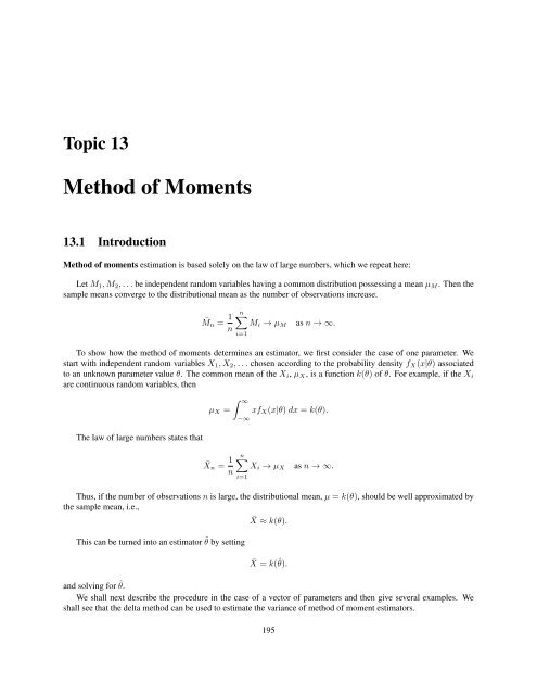
Topic 13<br />
<strong>Method</strong> <strong>of</strong> <strong>Moments</strong><br />
13.1 Introduction<br />
<strong>Method</strong> <strong>of</strong> moments estimation is based solely on the law <strong>of</strong> large numbers, which we repeat here:<br />
Let M 1 ,M 2 ,...be independent random variables having a common distribution possessing a mean µ M . Then the<br />
sample means converge to the distributional mean as the number <strong>of</strong> observations increase.<br />
¯M n = 1 n<br />
nX<br />
M i ! µ M as n !1.<br />
i=1<br />
To show how the method <strong>of</strong> moments determines an estimator, we first consider the case <strong>of</strong> one parameter. We<br />
start with independent random variables X 1 ,X 2 ,... chosen according to the probability density f X (x|✓) associated<br />
to an unknown parameter value ✓. The common mean <strong>of</strong> the X i , µ X , is a function k(✓) <strong>of</strong> ✓. For example, if the X i<br />
are continuous random variables, then<br />
µ X =<br />
Z 1<br />
xf X (x|✓) dx = k(✓).<br />
1<br />
The law <strong>of</strong> large numbers states that<br />
¯X n = 1 n<br />
nX<br />
X i ! µ X as n !1.<br />
i=1<br />
Thus, if the number <strong>of</strong> observations n is large, the distributional mean, µ = k(✓), should be well approximated by<br />
the sample mean, i.e.,<br />
¯X ⇡ k(✓).<br />
This can be turned into an estimator ˆ✓ by setting<br />
¯X = k(ˆ✓).<br />
and solving for ˆ✓.<br />
We shall next describe the procedure in the case <strong>of</strong> a vector <strong>of</strong> parameters and then give several examples. We<br />
shall see that the delta method can be used to estimate the variance <strong>of</strong> method <strong>of</strong> moment estimators.<br />
195
Introduction to the Science <strong>of</strong> Statistics<br />
The <strong>Method</strong> <strong>of</strong> <strong>Moments</strong><br />
13.2 The Procedure<br />
More generally, for independent random variables X 1 ,X 2 ,...chosen according to the probability distribution derived<br />
from the parameter value ✓ and m a real valued function, if k(✓) =E ✓ m(X 1 ), then<br />
1<br />
n<br />
nX<br />
m(X i ) ! k(✓) as n !1.<br />
The method <strong>of</strong> moments results from the choices m(x) =x m . Write<br />
i=1<br />
µ m = EX m = k m (✓). (13.1)<br />
for the m-th moment.<br />
Our estimation procedure follows from these 4 steps to link the sample moments to parameter estimates.<br />
• Step 1. If the model has d parameters, we compute the functions k m in equation (13.1) for the first d moments,<br />
µ 1 = k 1 (✓ 1 ,✓ 2 ...,✓ d ), µ 2 = k 2 (✓ 1 ,✓ 2 ...,✓ d ), ..., µ d = k d (✓ 1 ,✓ 2 ...,✓ d ),<br />
obtaining d equations in d unknowns.<br />
• Step 2. We then solve for the d parameters as a function <strong>of</strong> the moments.<br />
✓ 1 = g 1 (µ 1 ,µ 2 , ··· ,µ d ), ✓ 2 = g 2 (µ 1 ,µ 2 , ··· ,µ d ), ..., ✓ d = g d (µ 1 ,µ 2 , ··· ,µ d ). (13.2)<br />
• Step 3. Now, based on the data x =(x 1 ,x 2 ,...,x n ) we compute the first d sample moments,<br />
x, x 2 ,...,x d .<br />
Using the law <strong>of</strong> large numbers, we have that µ m ⇡ x m .<br />
• Step 4. We replace the distributional moments µ m by the sample moments x m , then the solutions in (13.2) give<br />
us formulas for the method <strong>of</strong> moment estimators (ˆ✓ 1 , ˆ✓ 2 ,...,ˆ✓ d ). For the data x, these estimates are<br />
ˆ✓ 1 (x) =g 1 (¯x, x 2 , ··· , x d ), ˆ✓2 (x) =g 2 (¯x, x 2 , ··· , x d ), ..., ˆ✓d (x) =g d (¯x, x 2 , ··· , x d ).<br />
How this abstract description works in practice can be best seen through examples.<br />
13.3 Examples<br />
Example 13.1. Let X 1 ,X 2 ,...,X n be a simple random sample <strong>of</strong> Pareto random variables with density<br />
f X (x| )= x<br />
+1 , x > 1.<br />
The cumulative distribution function is<br />
F X (x) =1 x , x > 1.<br />
The mean and the variance are, respectively,<br />
µ =<br />
1 , 2 = ( 1)2 ( 2) .<br />
196
Introduction to the Science <strong>of</strong> Statistics<br />
The <strong>Method</strong> <strong>of</strong> <strong>Moments</strong><br />
In this situation, we have one parameter, namely<br />
. Thus, in step 1, we will only need to determine the first moment<br />
µ 1 = µ = k 1 ( )=<br />
1<br />
to find the method <strong>of</strong> moments estimator ˆ for .<br />
For step 2, we solve for as a function <strong>of</strong> the mean µ.<br />
= g 1 (µ) = µ<br />
µ 1 .<br />
Consequently, a method <strong>of</strong> moments estimate for<br />
mean ¯X.<br />
is obtained by replacing the distributional mean µ by the sample<br />
ˆ =<br />
¯X<br />
¯X 1 .<br />
A good estimator should have a small variance . To use the delta method to estimate the variance <strong>of</strong> ˆ,<br />
we compute<br />
g 0 1(µ) =<br />
✓<br />
1<br />
(µ 1) 2 , giving g0 1<br />
2ˆ ⇡ g 0 1(µ) 2 2<br />
n .<br />
◆<br />
=<br />
1<br />
1<br />
(<br />
1<br />
1) = ( 1) 2<br />
2 ( ( 1)) 2 = ( 1)2<br />
and find that ˆ has mean approximately equal to<br />
and variance<br />
2ˆ ⇡ g 0 1(µ) 2 2<br />
n =( 1)4 n( 1) 2 ( 2) = ( 1)2<br />
n( 2)<br />
As a example, let’s consider the case with<br />
=3and n = 100. Then,<br />
2ˆ ⇡ 3 · 22<br />
100 · 1 = 12<br />
100 = 3<br />
p<br />
3<br />
25 , ˆ ⇡<br />
5 =0.346.<br />
To simulate this, we first need to simulate Pareto random variables. Recall that the probability transform states that<br />
if the X i are independent Pareto random variables, then U i = F X (X i ) are independent uniform random variables on<br />
the interval [0, 1]. Thus, we can simulate X i with F 1<br />
X<br />
(U i). If<br />
u = F X (x) =1 x 3 , then x =(1 u) 1/3 = v 1/3 , where v =1 u.<br />
Note that if U i are uniform random variables on the interval [0, 1] then so are V i =1 U i . Consequently, 1/ p V 1 , 1/ p V 2 , ···<br />
have the appropriate Pareto distribution.<br />
> paretobar for (i in 1:1000){v mean(betahat)<br />
[1] 3.053254<br />
> sd(betahat)<br />
[1] 0.3200865<br />
197
Introduction to the Science <strong>of</strong> Statistics<br />
The <strong>Method</strong> <strong>of</strong> <strong>Moments</strong><br />
Histogram <strong>of</strong> paretobar<br />
Histogram <strong>of</strong> betahat<br />
Frequency<br />
0 50 100 150 200 250<br />
Frequency<br />
0 50 100 150 200 250<br />
1.4 1.6 1.8 2.0<br />
paretobar<br />
2.0 2.5 3.0 3.5 4.0 4.5<br />
betahat<br />
The sample mean for the estimate for at 3.053 is close to the simulated value <strong>of</strong> 3. In this example, the estimator<br />
ˆ is biased upward, In other words, on average the estimate is greater than the parameter, i. e., E ˆ > . The<br />
sample standard deviation value <strong>of</strong> 0.320 is close to the value 0.346 estimated by the delta method. When we examine<br />
unbiased estimators, we will learn that this bias could have been anticipated.<br />
Exercise 13.2. The muon is an elementary particle with an electric charge <strong>of</strong> 1 and a spin (an intrinsic angular<br />
momentum) <strong>of</strong> 1/2. It is an unstable subatomic particle with a mean lifetime <strong>of</strong> 2.2 µs. Muons have a mass <strong>of</strong> about<br />
200 times the mass <strong>of</strong> an electron. Since the muon’s charge and spin are the same as the electron, a muon can be<br />
viewed as a much heavier version <strong>of</strong> the electron. The collision <strong>of</strong> an accelerated proton (p) beam having energy<br />
600 MeV (million electron volts) with the nuclei <strong>of</strong> a production target produces positive pions (⇡ + ) under one <strong>of</strong> two<br />
possible reactions.<br />
p + p ! p + n + ⇡ + or p + n ! n + n + ⇡ +<br />
From the subsequent decay <strong>of</strong> the pions (mean lifetime 26.03 ns), positive muons (µ + ), are formed via the two body<br />
decay<br />
⇡ + ! µ + + ⌫ µ<br />
where ⌫ µ is the symbol <strong>of</strong> a muon neutrino. The decay <strong>of</strong> a muon into a positron (e + ), an electron neutrino (⌫ e ),<br />
and a muon antineutrino (¯⌫ µ )<br />
µ + ! e + + ⌫ e +¯⌫ µ<br />
has a distribution angle t with density given by<br />
f(t|↵) = 1 (1 + ↵ cos t), 0 apple t apple 2⇡,<br />
2⇡<br />
with t the angle between the positron trajectory and the µ + -spin and anisometry parameter ↵ 2 [ 1/3, 1/3] depends<br />
the polarization <strong>of</strong> the muon beam and positron energy. Based on the measurement t 1 ,...t n , give the method <strong>of</strong><br />
moments estimate ˆ↵ for ↵. (Note: In this case the mean is 0 for all values <strong>of</strong> ↵, so we will have to compute the second<br />
moment to obtain an estimator.)<br />
Example 13.3 (Lincoln-Peterson method <strong>of</strong> mark and recapture). The size <strong>of</strong> an animal population in a habitat <strong>of</strong><br />
interest is an important question in conservation biology. However, because individuals are <strong>of</strong>ten too difficult to find,<br />
198
Introduction to the Science <strong>of</strong> Statistics<br />
The <strong>Method</strong> <strong>of</strong> <strong>Moments</strong><br />
a census is not feasible. One estimation technique is to capture some <strong>of</strong> the animals, mark them and release them back<br />
into the wild to mix randomly with the population.<br />
Some time later, a second capture from the population is made. In this case, some <strong>of</strong> the animals were not in the<br />
first capture and some, which are tagged, are recaptured. Let<br />
• t be the number captured and tagged,<br />
• k be the number in the second capture,,<br />
• r be the number in the second capture that are tagged, and let<br />
• N be the total population size,<br />
Thus, t and k is under the control <strong>of</strong> the experimenter. The value <strong>of</strong> r is random and the populations size N is the<br />
parameter to be estimated. We will use a method <strong>of</strong> moments strategy to estimate N. First, note that we can guess the<br />
the estimate <strong>of</strong> N by considering two proportions.<br />
the proportion <strong>of</strong> the tagged fish in the second capture ⇡ the proportion <strong>of</strong> tagged fish in the population<br />
r<br />
k ⇡ t N<br />
This can be solved for N to find N ⇡ kt/r. The advantage <strong>of</strong> obtaining this as a method <strong>of</strong> moments estimator is<br />
that we evaluate the precision <strong>of</strong> this estimator by determining, for example, its variance. To begin, let<br />
⇢ 1 if the i-th individual in the second capture has a tag.<br />
X i =<br />
0 if the i-th individual in the second capture does not have a tag.<br />
The X i are Bernoulli random variables with success probability<br />
P {X i =1} = t N .<br />
They are not Bernoulli trials because the outcomes are not independent. We are sampling without replacement.<br />
For example,<br />
P {the second individual is tagged|first individual is tagged} = t 1<br />
N 1 .<br />
In words, we are saying that the probability model behind mark and recapture is one where the number recaptured is<br />
random and follows a hypergeometric distribution. The number <strong>of</strong> tagged individuals is X = X 1 + X 2 + ···+ X k<br />
and the expected number <strong>of</strong> tagged individuals is<br />
µ = EX = EX 1 + EX 2 + ···+ EX k = t N + t N + ···+ t N = kt<br />
N .<br />
The proportion <strong>of</strong> tagged individuals, ¯X =(X1 + ···+ X k )/k, has expected value<br />
Thus,<br />
E ¯X = µ k = t N .<br />
N = kt<br />
µ .<br />
Now in this case, we are estimating µ, the mean number <strong>of</strong> recaptured with r, the actual number recaptured. So,<br />
to obtain the estimate ˆN. we replace µ with the previous equation by r.<br />
ˆN = kt<br />
r<br />
To simulate mark and capture, consider a population <strong>of</strong> 2000 fish, tag 200, and capture 400. We perform 1000<br />
simulations <strong>of</strong> this experimental design. (The R command rep(x,n) repeats n times the value x.)<br />
199
Introduction to the Science <strong>of</strong> Statistics<br />
The <strong>Method</strong> <strong>of</strong> <strong>Moments</strong><br />
> r fish for (j in 1:1000){r[j] Nhat mean(r)<br />
[1] 40.09<br />
> sd(r)<br />
[1] 5.245705<br />
> mean(Nhat)<br />
[1] 2031.031<br />
> sd(Nhat)<br />
[1] 276.6233<br />
Histogram <strong>of</strong> r<br />
Histogram <strong>of</strong> Nhat<br />
Frequency<br />
0 50 150 250 350<br />
Frequency<br />
0 50 150 250 350<br />
20 30 40 50 60<br />
r<br />
1500 2000 2500 3000<br />
Nhat<br />
To estimate the population <strong>of</strong> pink salmon in Deep Cove Creek in southeastern Alaska, 1709 fish were tagged. Of<br />
the 6375 carcasses that were examined, 138 were tagged. The estimate for the population size<br />
ˆN =<br />
6375 ⇥ 1709<br />
138<br />
Exercise 13.4. Use the delta method to estimate Var( ˆN) and<br />
Cove Creek data.<br />
⇡ 78948.<br />
ˆN<br />
. Apply this to the simulated sample and to the Deep<br />
Example 13.5. Fitness is a central concept in the theory <strong>of</strong> evolution. Relative fitness is quantified as the average<br />
number <strong>of</strong> surviving progeny <strong>of</strong> a particular genotype compared with average number <strong>of</strong> surviving progeny <strong>of</strong> competing<br />
genotypes after a single generation. Consequently, the distribution <strong>of</strong> fitness effects, that is, the distribution <strong>of</strong><br />
fitness for newly arising mutations is a basic question in evolution. A basic understanding <strong>of</strong> the distribution <strong>of</strong> fitness<br />
effects is still in its early stages. Eyre-Walker (2006) examined one particular distribution <strong>of</strong> fitness effects, namely,<br />
deleterious amino acid changing mutations in humans. His approach used a gamma-family <strong>of</strong> random variables and<br />
gave the estimate <strong>of</strong> ˆ↵ =0.23 and ˆ =5.35.<br />
200
Introduction to the Science <strong>of</strong> Statistics<br />
The <strong>Method</strong> <strong>of</strong> <strong>Moments</strong><br />
A (↵, ) random variable has mean ↵/ and variance ↵/ 2 . Because we have two parameters, the method <strong>of</strong><br />
moments methodology requires us to determine the first two moments.<br />
E (↵, ) X 1 = ↵ and E (↵, ) X 2 1 = Var (↵, ) (X 1 )+E (↵, ) [X 1 ] 2 = ↵ 2 + ✓ ↵<br />
◆ 2<br />
=<br />
Thus, for step 1, we find that<br />
↵(1 + ↵)<br />
2<br />
= ↵ 2 + ↵2 2 .<br />
µ 1 = k 1 (↵, )= ↵ , µ 2 = k 2 (↵, )= ↵ 2 + ↵2 2 .<br />
For step 2, we solve for ↵ and<br />
. Note that<br />
µ 2 µ 2 1 = ↵ 2 ,<br />
and<br />
So set<br />
to obtain estimators<br />
µ 1<br />
µ 1 ·<br />
µ 2 µ 2 1<br />
ˆ =<br />
¯X = 1 n<br />
µ 1<br />
µ 2 µ 2 1<br />
= ↵/<br />
↵/ 2 = ,<br />
= ↵ · = ↵, or ↵ = µ2 1<br />
µ 2 µ 2 .<br />
1<br />
nX<br />
X i and X 2 = 1 n<br />
i=1<br />
nX<br />
i=1<br />
X 2 i<br />
¯X<br />
X 2 ( ¯X)<br />
and ˆ↵ = ˆ ¯X (<br />
=<br />
¯X) 2<br />
2 X 2 ( ¯X) . 2<br />
dgamma(x, 0.23, 5.35)<br />
0 2 4 6 8 10 12<br />
0.0 0.2 0.4 0.6 0.8 1.0<br />
x<br />
Figure 13.1: The density <strong>of</strong> a<br />
(0.23, 5.35) random variable.<br />
201
Introduction to the Science <strong>of</strong> Statistics<br />
The <strong>Method</strong> <strong>of</strong> <strong>Moments</strong><br />
To investigate the method <strong>of</strong> moments on simulated data using R, we consider 1000 repetitions <strong>of</strong> 100 independent<br />
observations <strong>of</strong> a (0.23, 5.35) random variable.<br />
> xbar x2bar for (i in 1:1000){x mean(betahat)<br />
[1] 6.315644<br />
> sd(betahat)<br />
[1] 2.203887<br />
To obtain a sense <strong>of</strong> the distribution <strong>of</strong> the estimators ˆ↵ and ˆ, we give histograms.<br />
> hist(alphahat,probability=TRUE)<br />
> hist(betahat,probability=TRUE)<br />
Histogram <strong>of</strong> alphahat<br />
Histogram <strong>of</strong> betahat<br />
Density<br />
0 1 2 3 4 5 6<br />
Density<br />
0.00 0.05 0.10 0.15<br />
0.1 0.2 0.3 0.4 0.5<br />
alphahat<br />
0 5 10 15<br />
betahat<br />
As we see, the variance in the estimate <strong>of</strong> is quite large. We will revisit this example using maximum likelihood<br />
estimation in the hopes <strong>of</strong> reducing this variance. The use <strong>of</strong> the delta method is more difficult in this case because<br />
it must take into account the correlation between ¯X and X 2 for independent gamma random variables. Indeed, from<br />
the simulation, we have an estimate.<br />
> cor(xbar,x2bar)<br />
[1] 0.8120864<br />
Moreover, the two estimators ˆ↵ and ˆ are fairly strongly positively correlated. Again, we can estimate this from the<br />
simulation.<br />
> cor(alphahat,betahat)<br />
[1] 0.7606326<br />
In particular, an estimate <strong>of</strong> ˆ↵ and ˆ are likely to be overestimates or underestimates in tandem.<br />
202
Introduction to the Science <strong>of</strong> Statistics<br />
13.4 Answers to Selected Exercises<br />
13.2. Let T be the random variable that is the angle between<br />
the positron trajectory and the µ + -spin<br />
µ 2 = E ↵ T 2 = 1 Z ⇡<br />
t 2 (1 + ↵ cos t)dt = ⇡2<br />
2⇡ ⇡<br />
3<br />
⇡ 2 /3)/2. This leads to the method <strong>of</strong> mo-<br />
ˆ↵ = 1 ✓t<br />
2<br />
2 ⇡ 2 ◆<br />
3<br />
Thus, ↵ =(µ 2<br />
ments estimate<br />
2↵<br />
where t 2 is the sample mean <strong>of</strong> the square <strong>of</strong> the observations.<br />
y<br />
-0.3 -0.2 -0.1 0.0 0.1 0.2 0.3<br />
The <strong>Method</strong> <strong>of</strong> <strong>Moments</strong><br />
Figure 13.2: Densities f(t|↵) for the values <strong>of</strong> ↵ = 1<br />
(yellow). 1/3 (red), 0 (black), 1/3 (blue), 1 (light blue).<br />
-0.3 -0.2 -0.1 0.0 0.1 0.2 0.3<br />
13.4. Let X be the random variable for the number <strong>of</strong> tagged fish. Then, X is a hypergeometric random variable with<br />
mean µ X = kt<br />
N and variance 2<br />
X = k t N t N k<br />
N N N 1<br />
N = g(µ X )= kt . Thus, g 0 (µ X )= kt<br />
µ X µ 2 .<br />
X<br />
The variance <strong>of</strong> ˆN<br />
✓ ◆ 2<br />
Var( ˆN) kt<br />
⇡ g 0 (µ) 2 X 2 =<br />
µ 2 k t ✓ ◆ 2<br />
N t N k kt<br />
X<br />
N N N 1 = t kt/µ X t kt/µ X k<br />
µ 2 k<br />
X<br />
kt/µ X kt/µ X kt/µ X 1<br />
✓ ◆ 2 kt<br />
= k µ ✓ ◆ 2<br />
Xt kt µ X t kt kµ X kt<br />
= k µ X k µ X k(t µ X )<br />
kt kt kt µ X k k kt µ X<br />
µ 2 X<br />
= k2 t 2<br />
µ 3 X<br />
(k µ X )(t µ X )<br />
kt µ X<br />
Now if we replace µ X by its estimate r we obtain<br />
2ˆN ⇡ k2 t 2<br />
µ 2 X<br />
(k r)(t r)<br />
r 3 kt r<br />
For t = 200,k = 400 and r = 40, we have the estimate ˆN<br />
= 268.4. This compares to the estimate <strong>of</strong> 276.6 from<br />
simulation.<br />
For t = 1709,k = 6375 and r = 138, we have the estimate ˆN<br />
= 6373.4.<br />
.<br />
x<br />
203