The effect of correlation on the formation of clusters can ... - GreenBook

variables range from approximately -3 to + 4 in value, with mean
values <strong>of</strong> zero and standard deviations <strong>of</strong> one.
First, I conducted k-means cluster analysis using SAS
with variables X1 and X2. This method was chosen because it is
commonly used and well-understood. It uses Euclidean distance
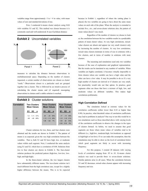
Exhibit 2 Uncorrelated variables
LH
LL
HH
LH
Panel 1
Panel 2
X 2 X 2
measures to calculate the distance between observations in
multidimensional space. Depending on the number <strong>of</strong> clusters
requested, a certain number <strong>of</strong> observations are chosen as cluster
“seeds.” Observations closest to a particular seed are grouped
together into a cluster. This is followed by an iterative process <strong>of</strong>
calculating the cluster means and (if required) reassigning
observations to clusters until a stable solution is reached.
Exhibit 3 Cluster solutions
Correlation Two Clusters Three Clusters Four Clusters
Mean Values Mean Values Mean Values
X1 X2 n X1 X2 n X1 X2 n
1.2 1.11 31% .34 -.30 63% -.17 -.14 46%
.91 -.49 -.49 69% -1.13 -1.13 29% -1.31 -1.33 21%
1.95 1.92 7% 1.04 .92 30%
2.32 2.32 3%
Cluster solutions for two, three, and four clusters were
obtained and the results are shown in Exhibit 3. <strong>The</strong> pattern <strong>of</strong>
means is as expected, given the very high <strong>correlation</strong> between the
variables. That is, both X1 and X2 have high, low, or moderate
values within each segment. Next, I conducted the same analysis
using X1 and X3, which have a <strong>correlation</strong> <strong>of</strong> 0.08. Solutions from
two to four clusters are shown in Exhibit 4. <strong>The</strong> four-cluster
solution produces the predicted pattern (high-low, low-low, lowhigh,
and high-high).
In the three-cluster solution, the two largest clusters
have substantially different means. <strong>The</strong> two-cluster solution isn’t
much different from the high <strong>correlation</strong> case, except for a slightly
higher difference between the means. This is to be expected
because in Exhibit 1, regardless <strong>of</strong> where the cutting plane is
placed, the two variables are going to have about the same mean
values on each side <strong>of</strong> the plane. When the analysis is extended to
include five-, six-, and seven-cluster solutions also, the pattern <strong>of</strong>
mean values doesn’t vary much.
Regardless <strong>of</strong> the number <strong>of</strong> clusters we choose to look
at, the <strong>correlation</strong> between the two variables results in a predictable
pattern <strong>of</strong> mean cluster values. At very high <strong>correlation</strong>s, mixedvalue
clusters are absent and appear (as very small clusters) only
by increasing the number <strong>of</strong> clusters. At very low <strong>correlation</strong>s,
mixed-value clusters dominate in terms <strong>of</strong> size in solutions with a
few clusters, and in terms <strong>of</strong> number in solutions with more
clusters.
<strong>The</strong> reasoning and simulations used only two variables
because <strong>of</strong> the ease <strong>of</strong> explanation and graphical representation.
But the results can be translated to any number <strong>of</strong> variables. When
variables are highly correlated, it becomes virtually impossible to
form clusters where one variable can have a high value and the
other can have a low value. It may be possible to do so if a very
high number <strong>of</strong> clusters are derived or if clusters are very small,
but practicality would rule out that option. In practice, good
segments <strong>of</strong>ten are those that have a mixture <strong>of</strong> high, low, and
moderate values on different variables. This makes high
<strong>correlation</strong>s problematic.
High Correlation Defined
<strong>The</strong> simulation looked at extreme values for the
<strong>correlation</strong> coefficients (either lower than 0.10 or higher than
0.90). In practice, what threshold values <strong>of</strong> <strong>correlation</strong> coefficients
may lead to problems in analysis One way to test this would be to
run simulations such as those described above with varying levels
<strong>of</strong> the <strong>correlation</strong> coefficients to observe the changes in the types
<strong>of</strong> clusters formed. As before, we need to assume that good
segments are those where mean values <strong>of</strong> variables tend to be
different (i.e., high/low, moderate/high, low/moderate as opposed
to high/high or low/low). If we can make this assumption, then the
simulations may be able to show us the level <strong>of</strong> <strong>correlation</strong> below
which good segments are likely to occur with increasing
frequency.
For this purpose, I created 20 datasets with varying
levels <strong>of</strong> <strong>correlation</strong> ranging from .95 to .01. K-means cluster
analysis was used to provide three- to seven-cluster solutions.
Similar patterns arise in all cases. When the <strong>correlation</strong> between
X1 and X2 decreases, mixed-value clusters appear with increasing
frequency and size.
Reprinted with permission from the American Marketing Association (Marketing Research, Vol 15, No. 1, Spring 2003)
19