document - NRSP

Options and Constraints
B.M. Campbell
S. Jeffrey
W. Kozanayi
M. Luckert
M. Mutamba
C. Zindi

Household Livelihoods
in Semi-Arid Regions:
Options and Constraints
B.M. Campbell
S. Jeffrey
W. Kozanayi
M. Luckert
M. Mutamba
C. Zindi

The Center for International Forestry Research (CIFOR) was established in 1993 as part of the
Consultative Group on International Agricultural Research (CGIAR) in response to global concerns
about the social, environmental and economic consequences of forest loss and degradation.
CIFOR research produces knowledge and methods needed to improve the well-being of forestdependent
people and to help tropical countries manage their forests wisely for sustained
benefits. This research is done in more than two dozen countries, in partnership with numerous
partners. Since it was founded, CIFOR has also played a central role in influencing global and
national forestry policies.
© 2002 by Center for International Forestry Research
All rights reserved. Published in 2002
Printed by SMK Grafika Desa Putera, Indonesia
Cover photos: B.M Campbell and Martin Hodnett
ISBN 979-8764-78-1
Published by
Center for International Forestry Research
Mailing address: P.O. Box 6596 JKPWB, Jakarta 10065, Indonesia
Office address: Jl. CIFOR, Situ Gede, Sindang Barang, Bogor Barat 16680, Indonesia
Tel.: +62 (251) 622622; Fax: +62 (251) 622100
E-mail: cifor@cgiar.org
Web site: http://www.cifor.cgiar.org

Contents
Acknowledgements
viii
Executive Summary
ix
Abstract 1
1. Introduction 3
2. The Study Sites 6
2.1 Location 6
2.2 History and population 6
2.3 Markets, infrastructure and services 8
2.4 Climate, agricultural potential, land use and risk 8
2.5 Institutional framework 11
2.6 The national economy 12
2.7 Why Chivi and why two case-study sites 13
3. Methods 14
3.1 Livelihood questionnaire data collection 14
3.2 Livelihood questionnaire data analysis 18
3.3 Participatory rural appraisal (PRA), participatory observation
and action research 21
3.4 Biophysical resource surveys and the geographical information system 21
3.5 Systems modeling 21
4. The wealth index and its variation 23
4.1 Creating the wealth index and wealth quartiles 23
4.2 Wealth quartile characteristics 24
5. Human, financial, physical and natural capital — the assets available
to households 25
5.1 Human capital 25
5.2 Financial capital 35
5.3 Physical capital 40
5.4 Natural Capital 41
5.5 Social capital 49
5.6 Reconstituting an integrated view of the assets of a household 53

Contents
6. Household productive activities — the generation of cash and subsistence
gross income 56
6.1 Dryland and garden production 56
6.2 Livestock production 63
6.3 Woodland use 68
6.4 Wages, remittances and home industry 73
6.5 Gross income patterns — summary, evidence of intensification
and change 77
7. Exploring household strategies 83
7.1 Quantitative analysis 83
7.2 Summarising the trends and patterns 86
8. Net income and poverty 89
8.1 Total net income 89
8.2 Poverty 90
8.3 Patterns of variation in components of net income 93
8.4 Building and balancing capitals to derive income and reduce risk 102
9. Temporal changes in livelihood strategies 104
9.1 Livelihood changes 104
9.2 Drivers of change 111
9.3 Dynamic livelihoods — where to 116
10Modelling livelihood change 118
10.1 The Bayesian Network approach and model structure 118
10.2 Main driving variables of vulnerability and cash income 118
10.3 Livelihood assets and markets 120
10.4 Raising cash income 122
10.5 Exploring livelihood improvements in dry years 122
10.6 Main conclusions from the Bayesian Network 124
11 Making a difference 125
11.1 The sustainable livelihoods perspective — should we be bolder 125
11.2 Resourceful farmers in a changing world 127
11.3 The causes of poverty and options to alleviate poverty 133
11.4 But, can rural development really make a difference 139
Endnotes 142
References cited 144
List of figures
Figure 1. Location of the two study areas in southern Zimbabwe 6
Figure 2. Mutangi Dam, used for small-scale irrigation, fishing and livestock watering 7
Figure 3. Annual rainfall at Chivi Business Centre 9
Figure 4. The view south-east from the top of the Romwe inselberg 10
Figure 5. Gently rolling landscape in Mutangi 10
Figure 6. Average time allocation (hours per day) for females, males and
children in 1999-2000 27
Figure 7. Average time allocation (hours per day) by females in the four
quarters of 1999-2000 29
Figure 8. Average time allocation (hours per day) by males in the four
quarters of 1999-2000 29
Figure 9. Average time allocation (hours per day) by children in the four
quarters of 1999-2000 29
Figure 10. Interactions between quarter and site for cash expenses for dryland crops 37
Figure 11. The relationship between acres of land owned for dryland crops and
household numbers for Romwe and Mutangi 43
Figure 12. Land-cover change in southern Zimbabwe 47
Figure 13. Vegetation types and land cover in Romwe and Mutangi
physical catchments 48
iv

Contents
Figure 14. The community garden in Romwe, supplied by hand-carried water
from the Chidiso collector well 57
Figure 15. Contribution to cash gross income by different dryland crops 59
Figure 16. Contribution to subsistence gross income by different dryland crops 59
Figure 17. Contribution to total gross crop income by different dryland crops 59
Figure 18. Contribution to cash gross income by different garden crops 60
Figure 19. Contribution to subsistence gross income by different garden crops 60
Figure 20. Contribution to total gross crop income by different garden crops 60
Figure 21. Women provide the bulk of labour for dryland cropping 61
Figure 22. A woman weeding a maize field with a cultivator drawn by oxen 64
Figure 23. Distribution of sampled households in Romwe 69
Figure 24. Sources of gross cash income 78
Figure 25. Sources of gross cash income by wealth quartile 78
Figure 26. Quarterly sources of gross cash income 79
Figure 27. Sources of gross cash and subsistence income by wealth quartile 80
Figure 28. The spatial distribution of livestock income in Mutangi 81
Figure 29. Similarities and differences among the household types,
as identified by principal components analysis 87
Figure 30. Sources of total (cash and subsistence) net income 91
Figure 31. Sources of net cash and subsistence income by wealth quartile 94
Figure 32. Sources of net cash and subsistence income by wealth quartile,
where wealth quartile is defined by net income, not assets 94
Figure 33. Sources of net cash and subsistence income by wealth quartile 95
Figure 34. Differences in average net income between sites per household
per year 96
Figure 35. Differences in average net income per household per year as
a function of gender of the household head 99
Figure 36. Differences in average net income per household per year as
a function of age of the household head 100
Figure 37. Differences in average net income per household per year as
a function of educational status of the household head 101
Figure 38. Differences in average net income per household per year as
a function of number of household members 101
Figure 39. Maize yield as related to annual rainfall for Zimbabwean
commercial farms, Zimbabwean communal areas and Chivi
communal area 107
Figure 40. Three decades of change in Chivi in (a) crop systems and
(b) livestock and woodcarving 108
Figure 41. The distribution of crops in fields in the central valley of
the Romwe micro-catchment in 1998/99 109
Figure 42. Percentage change in net income between 1993/94 and 1997/97
for Shindi Ward, Chivi 110
Figure 43. Items sold on the Masvingo-Beitbridge road made from
Afzelia quanzensis 112
Figure 44. The nodes and linkages of the Bayesian belief network 119
Figure 45. Changes in net cash income related to rainfall and the state of
the macro-economy 120
Figure 46. Options (each of the arrows) that can be used to improve cash
income status from the current state 123
Figure 47. The linkages of key variables determining wealth status 134
Figure 48. Watering day at the old garden at Mutangi Dam 137
v

Contents
List of tables
Table 1. Household survey structure 15
Table 2. Reconstruction of quarterly data 16
Table 3. Original sample of households in Romwe and Mutangi villages 16
Table 4. Sectors and activities for analysis of household livelihoods 18
Table 5. Proportions used to allocate ‘Agriculture General’ between
dryland crop production and gardening 19
Table 6. Distribution of Romwe and Mutangi households by wealth quartiles 24
Table 7. Differences in wealth indicators between Romwe and Mutangi 24
Table 8. Household composition by wealth quartile 26
Table 9. Education level by wealth quartiles 27
Table 10. Differences in labour per acre among wealth quartiles 28
Table 11. Differences in labour per acre among sites 28
Table 12. Differences in time use among wealth quartiles for males, females
and children 30
Table 13. Differences in mean leisure plus sleep time by quarter 32
Table 14. Differences in mean wage rates among quarters 32
Table 15. Number of paired activities with partial correlations 33
Table 16. Differences in expenditures on wages by quarters 34
Table 17. Differences in expenditures on wages among wealth quartiles 34
Table 18. Household cash expenses by sector 36
Table 19. Differences in expenses among quarters 36
Table 20. Differences in expenses among wealth quartiles 37
Table 21. Differences in expenses among sites 38
Table 22. Differences among wealth quartiles in percentage of households
with various assets 41
Table 23. Differences in household land holdings among wealth quartiles 43
Table 24. Differences in livestock ownership among wealth quartiles 45
Table 25. Differences among wealth quartiles in household access to
irrigation water 49
Table 26. Mean crop prices 58
Table 27. Average cash and subsistence gross income from crops per household
per year 58
Table 28. Differences among wealth quartiles in average gross income from
crops per household per year 61
Table 29. Differences between sites of average gross income per household
per year from crops 61
Table 30. Mean prices for livestock and livestock products 65
Table 31. Average cash and subsistence gross income from livestock
per household per year 65
Table 32. Differences in average gross income per household from livestock,
by quarters 66
Table 33. Differences in average gross income per household per year from
livestock, by wealth quartiles 66
Table 34. Differences in average gross income per household per year from
livestock, by site 67
Table 35. Mean prices for woodland products 69
Table 36. Average cash and subsistence gross income from woodlands
per household per year 70
Table 37. Differences in average gross income from woodlands per household,
by quarter 71
Table 38. Differences in average gross income from woodlands per household
per year, by wealth quartile 71
Table 39. Differences in average gross income from woodlands per household
per year, by site 72
vi

Contents
Table 40. Average gross income from wages/home industries and
remittances/gifts per household per year 74
Table 41. Differences in average gross income from wages/home industries
and remittances/gifts per household, by quarter 75
Table 42. Differences in gross income from wages and remittances among
wealth quartiles 75
Table 43. Differences in average gross income from wages and remittances
per household per year, by site 76
Table 44. Distribution of remittances by source and by quarter 76
Table 45. Distribution of remittances by source (with mean amounts per
payment in brackets) and by site — quarterly recall data 76
Table 46. Summary of the differences in gross income between sites and
wealth quartiles 81
Table 47. Household types and their distribution across wealth quartiles 84
Table 48. Average gross income per household per year by household types 85
Table 49. Percentage of households in a household type that obtain income
from a specified source 86
Table 50. Average cash and subsistence net income per household per year 90
Table 51. Analysis of covariance of net income variables 97
Table 52. Differences in average net income per household per year 98
Table 53. Livestock population dynamics for 1997-2000 for eight dip
tanks in southern Chivi 109
Table 54. Sensitivity analysis of ‘vulnerability’ for selected variables 121
Table 55. Sensitivity analysis of ‘vulnerability’ for selected variables,
with the rainfall regime and the macro-economic state held constant 122
List of boxes
Box 1. Some historical gossip — the settling of Chivi 7
Box 2. Ms Gradicy — Rearing chickens after accessing financial capital 39
Box 3. A successful cotton grower: The case of Mr Rusipe 39
Box 4. Mrs Chivaura, a productive vegetable producer 40
Box 5. Mr Mike — wood vendor 73
Box 6. Mr C. Kefasi and family — labouring for other farmers 74
Box 7. Mr J. Chivaura loses most children to migration 77
Box 8. The Dapani family — livestock owners 83
Box 9. Mr and Mrs Ncube — wage-earning, trading, gardening 84
Box 10. Mr Piteri — accumulation in the face of adversity 93
Box 11. Mrs F Mutadzi — successful intensive agriculturalist 99
Box 12. From rags to riches: the case of the Ranganayi family 115
Box 13. The Zigari family — struggling in the aftermath of death 117
Box 14. Opportunistic farming or desperation 131
vii

Acknowledgements
This publication is an output from projects funded by the UK Department for International
Development (DfID) and Swiss Agency for Development Cooperation for the benefit of
developing countries. Some support to Marty Luckert was made by ‘Agroforestry:
Southern Africa’ a project supported by the Canadian International Development Agency.
The views expressed are not necessarily those of the donors. The authors would
particularly like to thank the people of Romwe and Mutangi for their lengthy assistance
and participation in the research. The input and help of CARE is acknowledged, especially
that of Kelly Stevenson. For enlightening discussion on the complete overhaul of the
communal lands and the national economy we thank Dale Doré (Shanduko) and Ramos
Mabugu (Economics Department, University of Zimbabwe). We thank Sven Wunder (CIFOR)
for prompting us to critically evaluate the capital assets framework for understanding
rural livelihoods. We thank Peter Frost, Osiman Mabhachi, Alois Mandondo, Nonto
Nemarundwe, Bevlyne Sithole and Caroline Sullivan for their constant discussion and
support on the topics covered here. Comments on the text by Michael Drinkwater (CARE),
Ian Scoones (Institute of Development Studies) and two anonymous reviewers greatly
assisted us in completing this work. For his patience and excellent support we thank
Gideon Suharyanto for layout design.
viii

Executive summary
Questions. Our over-arching question is: What can the development community do, or
facilitate, to significantly improve livelihoods in semi-arid systems To answer this we ask:
What are the relative contributions of different sources of livelihood and how does this
vary amongst households To what extent are people constrained by their assets, including
labour availability How are livelihood portfolios changing What are the options to alleviate
poverty
Cases studies. We base our analysis on two case-study sites in the communal lands of
southern Zimbabwe – Romwe and Mutangi in Chivi. These are fairly typical, from a biophysical
perspective, of a vast domain of granite/gneissic landscapes in semi-arid areas of numerous
developing countries on three continents. Long-term mean annual rainfall is around 550-
600 mm and population densities 55-90 people/km 2 . The study areas are relatively well
positioned to markets — within 100 km of the provincial capital and close to smaller rural
markets. The woodlands and rangelands are part of the commons, while dryland fields
(maize predominant) and gardens are quasi-private. The latter are irrigated from
groundwater or surface water. Considerable responsibility for administration and resource
governance now resides with the district council, but de facto rules and regulations operative
at the village level are centred on traditional authorities. Our quantitative household survey
largely pre-dates the meltdown in the national economy that became increasingly grave
after 2000. From the specific characteristic of Romwe and Mutangi related to site and
history, we have derived general principles relevant to policy in semi-arid regions.
Methods and approach. Our main tool was a detailed livelihood questionnaire (with 24
visits per year to the sampled households). This survey yielded unique empirical results —
very few of the resource-use patterns recorded would be captured in standard household
budget surveys. The survey data were supplemented by participatory rural appraisal,
participatory observation (researchers and research assistants living in the community for
nearly three years), action research (some together with CARE), biophysical resource surveys,
a geographical information system and systems modelling. For the survey data, we identified
four equal-sized wealth quartiles based on household assets, using assets identified by
participatory wealth ranking. The systems model was produced as a means to integrate
different components of the project and as a means to integrate the different capital
assets and multiple livelihood strategies. To structure our research, we used the sustainable
livelihoods approach. While having many positive features, it is not without certain problems.
Capital assets. Human, financial, physical and natural assets are severely constrained
for most households. An analysis of rules, leadership and committee operations indicates a
system dominated by informal arrangements and the ineffectiveness of a number of
institutions.
ix

Executive summary
Human capital. After sleep and domestic activities, most time is spent on dryland cropping,
though on a per acre basis, gardening (mostly by women) is two times more labour intensive
than dryland cropping. Labour is generally fully utilised, without major under-utilisation
even in the dry season. Households make significant investments in education, in terms of
school fees, uniforms, school supplies and forgone labour. We focussed some attention on
the development of leadership in the action research, with good pay-off for one of the
community gardens (Chidiso), which was revitalised and expanded.
Financial capital. Households spend an average of Z$11,000 per year, with 80% of this
used for domestic needs. i Some households in Romwe were fortunate enough to have
received loans of between Z$500 and Z$3000 from a micro-credit scheme, representing a
major injection of cash. In a number of cases this resulted in some significant improvements
in livelihoods beyond the immediate cash injection, but the sustainability of the scheme is
open to question.
Physical and natural capital. The distribution of arable land appears to be the outcome of
a strong historical influence, with more recent arrivals having fewer assets. The local
traditional leaders allocate land, this being one way to gain recognition in the local social
arena. Over time, arable plots have been continually subdivided into small units as plot
owners pass on land to their grown-up sons. Given the lack of room for cropland expansion,
intensification is likely to increase as a response to land scarcity. However, HIV/AIDS is
threatening to change these scenarios. Government resettlement initiatives have not
reduced population pressures. Access to labour and labour-saving equipment allow
households to have larger field areas. One of the primary constraints to economic and
social development in these areas is the difficulty encountered in developing reliable
water supplies.
Social capital. There are numerous local norms about how behaviour within the society,
including those covering resources such as woodlands and water. Reciprocity is still strong,
though declining for some aspects. Rules wax and wane depending on the status of the
resource and the needs of the extractor. Committee functioning was shown to be far from
satisfactory, and the elite (largely traditional leaders and their relatives) dominate resource
management and use. The complexity of local organisations and power struggles is likely
to defy attempts by development projects to facilitate change. Development agencies
and scholars often equate the lack of strict enforcement of rules as evidence of institutional
failure. Institutional flexibility may lower transaction costs and cater for the shocks and
stresses that impinge on livelihoods.
Production and income
Production activities. Most households rely on income (cash and subsistence) from a
number of sources, including dryland crop production, gardening, livestock production,
woodland activities, wages or home industries and remittances/gifts. For dryland crops,
gross income is highest for, in order, maize, cotton, groundnuts and roundnuts. Major
garden crops are tomatoes and leafy vegetables (mostly rape). Draft, transport and milk
are the largest gross income sources from livestock. Woodland income largely comes from
fuelwood, structural items and wild foods. Remittances are mostly from urban areas in
Zimbabwe but also from South Africa and commercial farms/estates. Local wages are for
a wide range of jobs and there is also a diversity of home industries. All activities are
deeply embedded in local social processes (e.g., for gardens this involves negotiating
water use and, in the community gardens, many decisions related to crop production).
Net incomes — subsistence and cash. On average, dryland crops contribute 22% of total
net income (cash and subsistence), gardens 8%, livestock 21%, woodlands 15%, wages and
home industries 12% and remittances and gifts 21%. About 45% of total net income is cash
x

Executive summary
income. Very little of the total net income for dryland crops, livestock and woodlands is
cash (only 21%, 8% and 10% respectively), but for garden crops half is cash (54%). It is clear
that income from wages/home industries and remittances/gifts is particularly important
for cash income generation (73% of total cash income), with only 10% of cash derived from
dryland crops. It is during the dry season from June to November that households are
especially constrained by cash.
Differentiation and the determinants of income
The assets — a gloomy prognosis. The capital endowments and production activities of
households interact to determine the well-being outcomes of households. A major
determinant of dryland crop production income is cattle numbers, as these provide inputs
into cropping (manure and draft), but access to non-farm cash income also improves crop
income, as it is a major source of cash to purchase inputs. For garden production, the
important variable is access to land for irrigation, while remittance income is probably the
main variable determining improved livestock income, as remittances are used to purchase
cattle. Lack of access to cash income drives some households into sales of woodland
products and larger wage/home industry incomes are associated with higher educational
status. Given low capital endowments, there are limitations on what a household can
produce. We found many limitations in the ability to expand natural capital. Labour is fully
utilised and undertaking secondary education is in decline. The state is continuing to
withdraw from its service role (education, extension, health, veterinary). Injections of
cash from the agricultural output of the previous cropping season are limited to a small
sub-population of the communities that have specific characteristics (e.g., access to cash
for inputs, access to fields with particular soil characteristics).
Axes of differentiation. Inevitably, there are different types of households, with different
livelihood strategies and different patterns of resource use. The major axes of differentiation
are those related to gender, wealth and site. We can identify 10 household types (based on
income levels and different activities). Differences between these are largely the result of
the levels of income that various activities bring, rather than qualitatively different activities.
Thus, differentiation is not as marked as in many other rural locations around the globe. It
is apparent that our asset-based wealth class is the most important differentiating variable
(as compared to others such as sex of the head of household, ethnic group, etc.). One
factor driving differentiation is whether a household has access to remittance income,
which can be reinvested in farming activities (especially livestock and cash crops) and
education, two variables which can further change household status.
Wealth differentiation. Marked wealth differentiation occurs, with local people recognising
the different wealth groupings largely on the basis of various capital assets. There is marked
inequity in access to assets (e.g., 20% of households own 61% of the overall cattle herd). We
see wealthier households committing more funds to building human capital and to purchasing
physical assets. Not only do wealthier households have more labour units, they also devote
more time to productive activities and academic pursuits, as well as hiring more labour. The
relative proportion of net income from different sources indicates clearly how the assetbased
wealth quartiles rely on a different spectrum of activities. Income from dryland and
subsistence crops never exceeds 25% of total income, with the higher proportions in the
wealthier households. About 30-35% of income is cash from wages/home industries and
remittances in all wealth quartiles, with remittances proportionally more important in
wealthier households and wages/home industries in poorer quartiles. Poorer households
receive only 7% of total income from livestock, but this is 25% in wealthier households.
Woodlands show the opposite pattern with 28% in poorer households and 9% in the wealthier
groups. The lowest quartile is particularly dependent on wages as a source of cash. The top
quartile is the only one in which households derive more than one-third of their gross cash
income from crops, but their main source of cash income is remittances.
xi

Executive summary
Site differences — patterns of intensification. We can identify greater intensification
(measured as inputs per unit area) and monetisation in Romwe, with more purchased
and in-kind inputs, closer livestock-crop integration and greater cash outputs. This may
be due to the closer proximity of Romwe to a market (Ngundu Halt), but it may also be
due to the better cropping potential and/or higher population densities in Romwe (with
resulting greater land scarcity). On the other hand, the cash market for woodland products
is better developed in Mutangi, where woodland resources are less plentiful. The patterns
of increased intensification do not lead to any degree of poverty alleviation in Romwe;
in fact, Mutangi, on average, may be in a slightly better position as a result of its lower
cash input costs.
Gender. Males spend 18% less time on productive work than females. Women have less
time for leisure and almost none of their time is devoted to academic activities. On the
agricultural side, men focus on livestock and dryland cropping, while women focus on
gardening and dryland cropping. We see the ruling elite, dominated by men, having a
strong control over the activities of the community. However, in a number of cases there
are some powerful women also wielding considerable power. There has been an upsurge
of trading activity, much of it conducted by women.
Drivers of change. Elements of change can be identified in numerous aspects of
capital assets and livelihood strategies. We suggest that there are some key drivers of
change, namely: (a) rainfall, (b) macro-economic changes, (c) changing institutional
arrangements and social processes, and (d) demographic processes and HIV/AIDS.
Rainfall. Rainfall is a primary driver of change, altering crop production from year to
year and causing massive longer-term fluctuations in livestock numbers. Households are
unable to raise sufficient grain for their subsistence needs in one out of three years. In
particularly bad droughts, or as a result of a sequence of bad years, water reserves are
reduced and garden production is also affected, with preference for water use given to
watering livestock (not without contest and conflict). Droughts are great reducers of
inequality, with the largest absolute losses in income in post-drought periods incurred by
the farmers with many cattle. However, these farmers also have a great deal of resilience,
and are usually in a better position to build up the herd again.
Macro-economic changes. Smallholder farmers are linked to the national economy
through remittances derived from other sectors of the economy, prices of agricultural
inputs and products, and services provided by government. Between 1993/94 and 1996/
97, when structural adjustment was being implemented, remittance income increased
in neighbouring Shindi Ward, but now the national economy is undoubtedly shrinking and
remittance income is, by numerous local accounts, in decline. Terms of trade have also
changed over the last few years, with a resulting drastic decline in groundnut and roundnut
cultivation and increased maize and cotton production (though the recent downturn in
the national economy has seen cotton production reduced). There has also been a shift
from food crops to cash crops, at least in the top wealth quartile. Liberalisation of the
exchange rate saw an influx of tourists into Zimbabwe in the 1990s, fuelling the woodcraft
market. Liberalisation also led to some other positive changes for rural people, e.g., a
flourishing informal trade. One negative impact of structural adjustment, as implemented
in Zimbabwe, has been the rolling back of government services in rural areas, including
the previously free health and education services, agricultural extension and veterinary
services. Cash is at a premium — we calculate that cash income stands at less than
US$0.20 per person per day. The need to raise cash and the reduced rates of out-migration
by young males to formal jobs is having repercussions throughout the livelihood system.
Many of the changes we see can be linked to these processes — increased monetisation,
changing gender relations, changing social norms, diversification into non-farm activities
and greater differentiation.
xii

Executive summary
Changing institutional arrangements and social processes. At the country/regional
level, the enforcement of some national environmental laws has been all but halted,
resulting in an upsurge of gardening and the widespread sale of forest products.
Traditional leaders remain central to daily village life and they are behind many
important decisions that influence the livelihoods of villagers, but their powers are
being challenged and traditional rules are not as strictly adhered to. These leaders
will often turn a blind eye to some activities that transgress the local rule system
citing the dire economic situation that their subjects face. Younger men, now more in
evidence in the community as a result of declining external opportunities, are also
forces for change — challenging the authority of the older men and the elites. Reciprocity
is still important but cash is governing more transactions amongst households. At the
household level, women are moving into new activities, such as trading, which involves
them moving temporarily away. Changing mores are also noted — petty theft, which
was once seldom heard of, is now more frequent.
Demographic processes and HIV/AIDS. With the slowly rising populations, the lack of
jobs in the formal sector for young men, and the limited land redistribution in Zimbabwe
not providing opportunities for people such as those in Chivi, endowments of natural
capital — land, livestock, common land for grazing and woodland products — continue
to decline. These are factors set to drive intensification. However, most of the
quantitative data that we have compiled on temporal change illustrate trends that are
much more rapid than the demographic changes that are taking place. Thus most of
the changes we discern cannot be primarily attributed to population increases. In the
study areas there has been an unprecedented rise in deaths linked to the HIV/AIDS
pandemic. This has had negative impacts on remittances (and all the ensuing effects
on education and crop and livestock production) and labour availability, has increased
the cash diverted to medical and death expenses, and has even increased the slaughter
of cattle. Unexpected impacts are a reduced willingness/ability to attend developmentoriented
meetings because of other demands on time (e.g., attending funerals, work
to maintain household income).
Resourceful farmers in a changing world
Resourcefulness. The study suggests that households have a rich and varied livelihood
portfolio, with displays of infinite resourcefulness to make ends meet. Patterns of
livelihood change over time, with their concomitant changes in institutions, illustrating
the responsiveness of farmers and the community to external signals, and their
resourcefulness despite the low levels of capital assets. Who would have predicted in
the 1980s that within the next decade there would be a minor gold rush, an
unprecedented upsurge in woodcarving, a flourish of trading activity and a new migration
to South Africa Many past interpretations of communal areas in Zimbabwe, as elsewhere
in Africa, have followed neo-Malthusian reasoning, but we find little evidence for a
downward spiral of communities triggered by rapid population growth. The neo-
Boserupian perspective, on the other hand, is clearly enviro-optimistic and also tends
to be livelihood optimistic. We do not see the poverty status of rural households changing
fundamentally in semi-arid regions, as part of the neo-Boserupian processes, if indeed
such processes are occurring.
A conceptual model of change. Any simple model of change, e.g., that of Boserup,
may give us some useful insights but is severely limited when confronted with the
complexity of rural production systems, with their multiple pathways of change and
multiple causalities. Following Mortimore and Benjaminsen, we suggest that a more
appropriate model of such systems is that they are non-equilibrial and opportunistic;
they are systems in constant transition. Elements of the system can display long-term
changes in slow variables (e.g., population growth, reduction of ‘sacredness’ of
landscape features), rapid directional (at least for a certain period of time) changes in
xiii

Executive summary
fast variables (e.g., rapid expansion of production of a specific crop such as cotton in
response to specific market signals), fluctuations in responses to some determinants
(e.g., rainfall) and reversals of states (e.g., loss of a breadwinner from HIV/AIDS causing
a household to move from the wealthiest quartile to a very poor quartile). Different
households, depending on their capital assets, will be moving in different directions.
Rural economies and societies appear as a shifting kaleidoscope of activities, household
types, conflicts, alliances and manoeuvres, in which it is difficult to discern the direction
a particular household type will next take, who is in control, the next strategy and the
impact on the asset base.
Poverty — can we make a difference
Poverty status. Seventy per cent of the households fall below the food poverty line, ii
while 90% fall below the consumption poverty line, iii indicating the pervasive poverty
that exists. De facto female-headed households (households where the male is working
away from the homestead) are shown to be better off than de jure female-headed
households (widows or unmarried/divorced women) or male-headed households. This
reinforces the importance of remittances to uplift a household, as de facto femaleheaded
households have high remittances. Development agencies generally try to focus
on the poorest of the poor — in the case of Chivi, and many similar semi-arid systems,
the bulk of the population could be considered prime targets for interventions. Even
the wealthiest quartile has a mean income of less that US$1 per day per person.
Households with large remittance and cash crop incomes can escape poverty. Cattle
numbers, size of dryland fields and educational levels are also correlated with poverty
status. Thus access to assets is important in determining poverty levels. This is probably
a self-reinforcing cycle with access to assets allowing households to improve income,
and hence to reinvest in further assets. Case-study interviews indicate a general
consensus that the richer are getting richer, while the poor are getting poorer; thus
differentiation is thought to be increasing.
The causes of poverty, and the need for integrated approaches: Rural poverty in
semi-arid regions is a result of a combination of interacting social, economic and
environmental factors and processes operating at a range of scales. Some of these are:
(i) adverse biophysical conditions, resulting in, among other things, low agricultural
potential and disastrous crashes in livestock numbers; (ii) insufficient high-quality
land, which is a result of colonial land-allocation patterns; (iii) labour scarcities, even
more so in the face of the HIV/AIDS pandemic; (iv) economic remoteness, with
presumably higher transaction and input costs, and few investments because returns
to investments are low compared to other places; (v) lack of credit markets as a result
of little or no collateral; (vi) few employment opportunities and low levels of education
and skill; (vii) low incomes and hence an inability to purchase some basic needs (e.g.,
medicines, secondary school education); (viii) poor macro-economic conditions; (ix)
the HIV/AIDS pandemic, resulting in the loss of breadwinners, labour scarcities and
increased costs; (x) low levels of empowerment; and (xi) declining woodland resources
leading to the need for greater investments (e.g., labour) to acquire basic products.
The multi-faceted nature of poverty indicates that there is no silver bullet to rural
development, and that an integrated, multi-sectoral approach to development is
critical, with different but complementary activities across a wide range of sectors.
Environment-poverty nexus. Considering that livestock income is largely based on rough
grazing, the common pool resources of the woodlands and grazing areas provide 30-40%
of net income for all wealth quartiles, with this income being predominantly grazing for
the top wealth quartiles and forest products for the lowest quartile. In these landscapes
water can also be classed as a predominantly common pool resource — it is essential for
garden production, which contributes nearly 10% of total income in all quartiles. Thus
common pool resources form the basis for between one-third and one-half of all income.
xiv

Executive summary
Given their contribution to household livelihoods, it is surprising the extent to which
some analysts disregard these resources, the focus often being on dryland crop
production. There is some evidence that woodlands are degrading and, from a technical
perspective, a higher degree of management of the herd size would probably lead to
greater financial return from grazing lands, but the transaction costs of achieving
management of a common pool resources are presumably very high. In general, we
recognise that there are very low incentives to manage natural resources in the
commons, and there are almost no technical or institutional interventions that could
be used to change this situation. Removing ineffective national- and district-level
regulations related to woodlands and grazing areas, and empowering local leaders,
will be a step in the right direction. Given that households are mostly well below the
poverty line, and that forest products (here we exclude grazing) are more important
to the poorest groups, we consider forest resources to be a safety net, preventing
households from even slipping further into poverty. For a few individuals (e.g., the
master carvers) woodlands may be more than a safety net.
Interventions. Our main conclusions, through statistical analysis of the livelihood data,
systems modelling and action research were that: (i) an integrated approach, covering
several production activities, is required to make any sizeable impact on income; (ii)
building the capacity of organisations can be as important, if not more so, than any
focus on a particular production system; (iii) market development is critical to improved
cash income; and (iv) macro-economic impacts on local livelihoods outweigh the effects
that can be achieved through local development initiatives. Of paramount importance
is the development of an enabling policy environment in which indigenous capital can
be effectively mobilised and the merits of technological options can be explored by
the farmers themselves. Support through the provision of market information and the
development of marketing organisations will allow households to respond positively to
markets, and thus to drive development themselves. A variety of possible intervention
points are identified.
But, can rural development really make a difference The donor community has set
an ambitious target for poverty alleviation in developing countries — the reduction of
people living in extreme poverty by half between 1990 and 2015. We can identify rural
development options to improve livelihoods but the impact, in terms of lifting people
beyond an income of US$1 per day, will be limited. Our overall conclusion is that there
are very few options for significantly improving livelihoods in semi-arid regions and
that the poverty alleviation targets set by the international community are overly
ambitious. Our analyses suggest that rainfall variation and the state of the macroeconomy
are likely to have a greater impact on livelihood status than any intervention
at the local level. We suggest that for real poverty alleviation we have to look forward
to the day without communal lands! The pre-condition for this (or even only a portion
of this dream), however, is very high growth rates in the manufacturing and service
industries driven by high investment levels to create the necessary additional
employment. This, of course, presumes a conducive political climate, macro-economic
stability and good luck: good rains, buoyant commodity prices, lowering trade barriers,
and so on. Rural development is only one small part of alleviating poverty.
i
US$1 = Z$38-40 at the time of the study.
ii
The food poverty line represents the income required to meet basic nutritional needs.
iii
The consumption poverty line allows for basic food consumption and some spending for housing, clothing,
education, health and transport.
xv

Household Livelihoods
in Semi-Arid Regions:
Options and Constraints
Campbell, B.M. 1
Jeffrey, S. 2
Kozanayi, W. 3
Luckert, M. 2
Mutamba, M. 3
Zindi, C. 2
Abstract
The overall aim of this study was to explore what the development community can do,
or facilitate, to significantly improve livelihoods in semi-arid systems. We based our
analysis on two case-study sites in the communal lands of southern Zimbabwe, areas
fairly typical of a vast domain of granite/gneissic landscapes in semi-arid areas of
numerous developing countries on three continents. Our main tool was a detailed
livelihood questionnaire, supplemented by participatory appraisal and observation,
action research, biophysical analysis and systems modelling. Human, financial, physical
and natural assets are severely constrained for most households. An analysis of rules,
leadership and committee operations indicates a system dominated by informal
arrangements, and the ineffectiveness of a number of institutions. Most households
rely on cash and subsistence income from a number of sources — dryland crop
production, gardening, livestock production, woodland activities, wage or home
industries and remittances/gifts. Marked wealth differentiation occurs, with local
people recognising the different wealth groupings largely on the basis of various capital
assets. One factor driving differentiation is whether a household has access to
remittance income. The wealthiest quartile is the only one in which households derive
more than a third of their gross cash income from crops, but their main cash income is
remittances. Elements of change can be identified in numerous aspects of the capital
assets and the livelihood strategies. We suggest that there are some key drivers of
change, namely: (a) rainfall, (b) macro-economic changes, (c) changing institutional
arrangements and social processes, and (d) demographic processes and HIV/AIDS. The
study suggests that households have a rich and varied livelihood portfolio, with displays
1

Abstract
of infinite resourcefulness to make ends meet. We found little evidence of a downward
spiral triggered by rapid population growth, but we do not see the poverty status of
rural households improving in semi-arid regions, as part of intensification processes.
Most households fall below various internationally recognised poverty lines. Rural poverty
is the result of a suite of interacting social, economic and environmental factors and
processes operating at a range of scales. The multi-faceted nature of poverty indicates
that there is no silver bullet to rural development, and that an integrated, multisectoral
approach to development is critical, with different, but complementary,
activities pursued at different levels. We recognise that there are very low incentives
to actively manage natural resources in the commons, and there are almost no technical
or institutional interventions that could be used to change this situation. Removing
ineffective national- and district-level regulations related to woodlands and grazing
areas, and empowering local leaders, will be a step in the right direction. In pursuing
poverty reduction, of paramount importance is the development of an enabling policy
environment to allow farmers to experiment and capture opportunities. Our overall
conclusion is that there are very few options for significantly improving livelihoods in
semi-arid regions and that the poverty alleviation targets set by the international
community are overly ambitious. Our analyses suggest that rainfall variation and the
state of the macro-economy are likely to have a greater impact on livelihood status
than local rural development interventions.
2

1. Introduction
This book is about the challenges and constraints rural households face in living in
semi-arid areas, and the role of development in alleviating poverty. Foremost among
the challenges are the often-marginal environmental conditions for many forms of
agriculture, created by low and erratic rainfall, frequent droughts and generally poor
soils (Scoones et al. 1996; Mortimore 1998; Frost and Mandondo 1999). Surface and
groundwater supplies are often poorly developed, unreliable or contaminated by
livestock. Access to good-quality agricultural land is often limited, sometimes by high
population densities (e.g., Malawi) or by the alienation of better farming land for
large-scale commercial concerns (e.g., Zimbabwe). Chronic food shortages are
widespread. For instance, almost 54% of the population in the districts of Chiredzi,
Beitbridge and Chivi in southern Zimbabwe requested food aid each year during the
period 1982-1993 (Frost and Mandondo 1999).
The risk and uncertainty associated with semi-arid regions, in particular the
recurrence of drought and the frequency of crop failure, means that farmers adopt
risk-averse strategies (Scoones et al. 1996; Mortimore 1998; Frost and Mandondo
1999). Such strategies, placed in the context of high livestock and human populations,
may encourage heavy dependence on the environment. Rural communities depend on
a wide range of natural products to supplement their livelihoods, most of them derived
from the commons (Bradley and Dewees 1993; Braedt and Standa-Gunda 2000).
Weakness of local institutions and high transaction costs, however, make it difficult to
manage common pool resources as new pressures emerge (Campbell et al. 2001b).
Environmental problems include deforestation, overgrazing of rangelands and increased
soil erosion, though there is much debate as to the severity, causes and impacts on
livelihoods (Whitlow 1980; Whitlow and Campbell 1989; Bradley and Dewees 1993;
Timberlake et al. 1993; Scoones et al. 1996; Campbell et al. 1997a; Mortimore 1998).
Whereas agricultural production is constrained primarily by the low potential of
much of the land, it is also affected adversely by a range of socio-economic factors
(Frost and Mandondo 1999). It is almost impossible for farmers to secure the credit
and loans needed to purchase agricultural inputs. Markets are under-developed and
often difficult to access consistently because of long distances, cost of transport and
sometimes poorly developed and maintained infrastructure. Access to appropriate
extension advice is minimal. Institutional arrangements governing resource use may
not function efficiently, to the detriment of local livelihoods and the environment.
Many people, mostly men, are attracted by paid employment outside the rural
areas, leaving women with the burden of production. Labour scarcities are being further
compounded by the rising number of deaths as a result of HIV/AIDS (World Bank 1996).
The contribution to household economies of income derived from employment, returned
through remittances, may be declining, because of stagnating and declining economies
in the region (Addison 1996; World Bank 1996; Arrighi 2002). Livelihoods are also
vulnerable to economic policy shifts, particularly economic reform programmes whose
3

HOUSEHOLD LIVELIHOODS IN SEMI-ARID REGIONS
pressures reinforce dependence by the poor on the environment, often causing further
rapid deterioration in its quality (Chipika and Kowero 2000).
In our study we investigate livelihood activities, in the context of natural resources
and their use, and explore how development initiatives might influence the relative
poverty or affluence of the people. We focus on two nearby sites in southern Zimbabwe.
While the sites have many peculiarities dictated by space, time and history, the central
themes are of wide interest to researchers and practitioners in semi-arid regions.
These themes cover the causes and consequences of poverty, the drivers of livelihood
changes, the importance of external factors in controlling local livelihood outcomes
and the role of rural development practitioners in promoting change. All too often
rural studies are too narrow, ignoring the wider dynamics of society, politics and the
economy, and failing to take history into account. Our focus on the details of survey
data from the two sites could lead to this same myopia, at least in print in such a book,
with us getting lost in the means, standard errors and significance tests. Here we do
describe much of the survey data collected, as the book is the descriptive account of
the bulk of our data — in subsequent publications, led by Chris Zindi and Sibongile
Moyo, we will be taking components of the data and providing more in-depth and more
sophisticated analyses (largely using mathematical programming and econometric
models based on utility maximisation). While we do provide some qualitative data in
this book, the project has produced a series of publications that focus on qualitative
insights regarding livelihoods and social processes (Mandondo et al. 2002; Nemarundwe
2002a,b,c; Nemarundwe and Kozanayi 2002; Sithole et al. 2002).
Our over-arching question is: What can the development community do, or
facilitate, to significantly improve livelihoods in semi-arid systems The donor
community has set an ambitious target for poverty alleviation in developing countries
— the reduction of people living in extreme poverty by half between 1990 and 2015
(World Bank 2001). Can rural development practitioners make a major contribution to
this goal Despite decades of investment in rural development initiatives, poverty is
widespread in sub-Saharan Africa, with no signs of significant reduction (Berry 1993).
Scoones (1994), writing on pastoral development in Africa, notes that all is not well in
the drylands of Africa, citing recurrent drought, civil war and economic decline as
characterising too many of the drylands. An appalling record of previous governments
in supporting pastoral development has convinced donors and governments that further
investment will be of little value. However, he suggests that there is growing consensus
of a new approach. Chambers (1994) abounds with optimism, citing the elements of a
professionalism that will rise to the challenges and opportunities emerging from farmers’
realities. Elements of this professionalism include taking risks, embracing errors and
learning; developing, adopting and spreading new methods and approaches; forming
new alliances and associations; articulating a vision of an agriculture based on
participation and equity; and working to make that vision a reality, with poor farmers
gaining more say and playing more of a role in rural development. While we agree that
there are new approaches and insights that can drive our rural development initiatives,
this book examines whether there is any room for optimism in relation to our goal of
significantly changing poverty levels through rural development.
The specific objectives and key questions of our study are:
• To identify the different groups of resource users and quantify their dependence
on each class of resource relative to the other components of their livelihoods.
What are the relative contributions of different sources of livelihood In
particular, to what extent does agriculture play a role in subsistence and cash
income generation, as compared to forest products and non-farm income What
role do common property resources play in the livelihood portfolios of people
in semi-arid regions Inevitably, there are different types of households, with
different patterns of resource use (Scoones 1995; Cavendish 1999a, 2002a,b).
What is the pattern of differentiation among households What is driving
differentiation To what extent are people constrained by labour availability
4

Introduction
Labour is generally in short supply in smallholder semi-arid systems (Berry 1993;
Mortimore 1998). We also ask how HIV/AIDS may be influencing labour availability
(and livelihoods more generally). We consider the social processes that mediate
supply of labour.
• To analyse how livelihood portfolios are changing. Available evidence suggests
continuing livelihood diversification, increased monetisation and constantly
shifting livelihoods (Bryceson 1996, 2000, 2002; Scoones et al. 1996; Ellis 1998,
1999, 2000; Mortimore 1998; Ashley and Maxwell 2001; Orr and Mwale 2001).
We examine whether this is the case, exploring whether there is any evidence
of poverty reduction, and look at the drivers of change. Change and adaptation
are central themes in the study of semi-arid livelihoods (Scoones 1994; Scoones
et al. 1996; Mortimore 1998), with common drivers being variable rainfall,
changing market conditions and the complex of factors driving intensification
and monetisation of production (Boserup 1965; Mortimore 1998; Bryceson 2000).
The use of water for economically productive purposes is part of a wellestablished
progression of gradual intensification of farming systems (Boserup
1965).
• To identify options that are likely to significantly improve the livelihoods of
people. From the perspective of external agents, is the integrated management
of livelihood assets a means to eliminating rural poverty DFID NRRD (1998)
suggests that the sustainable livelihoods approach (Carney 1998) needs to be
tested and transformed into practice. DFID NRRD (1998) go on to suggest that
one approach to development is to improve the understanding of the asset
base of a particular rural system and then develop a suite of options for
interventions. We embraced the sustainable livelihoods perspective to derive
our conceptual model of the system and to frame the way we undertook our
work. We reflect on the value of the approach as a means towards poverty
alleviation. We are particularly concerned that rural development initiatives,
centred on natural resource use, may not lead to significant poverty reduction
(Wunder 2001). The value of natural resources as a component of livelihoods is
undeniable (e.g., Cavendish 2002b), but this does not imply that natural
resources will provide the means to poverty alleviation. The constraining
biophysical conditions in semi-arid regions, particularly low and unreliable
rainfall, may severely limit the ability of households to mobilise resources and
improve incomes. In addition, the lack of reliable markets may limit the ability
of households to intensify production and benefit from cash crops. It is these
themes that we address in this book.
In Chapter 2 we give a background to the study sites in southern Zimbabwe. This
is followed by a description of the methods (Chapter 3). In Chapter 4 we derive a
household wealth index and briefly describe its variation between the study areas.
The index is based on indicators of wealth (e.g., cattle numbers). In the fifth chapter
we analyse the resources that can be utilised for productive activities: human, financial,
physical and natural capital. In Chapter 6 we investigate gross income in the various
sectors of household activity: crop production, livestock production, woodland
production, wages/home industries and remittances/gifts. Chapter 7 explores
differentiation amongst households. Chapter 8 describes how net income varies amongst
households. It also explores the poverty status of households. Chapter 9 summarises
the temporal dynamics in household livelihoods. Chapter 10 explores the likely impacts
of different development options on cash income using a systems modelling approach.
Chapter 11 concludes with our responses to the questions about whether the sustainable
livelihoods approach is valuable as a means to poverty reduction, and whether the
development community can substantially improve livelihoods in semi-arid regions.
5

2. The Study Sites
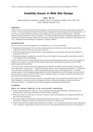
Figure 1. Location of the two study areas in southern Zimbabwe
2.1 Location
The work was conducted at two sites in Chivi District of Masvingo Province in
southeastern Zimbabwe. The study areas were the villages of Romwe (20 o 45’S, 30 o 46’E)
and Mutangi (20 o 15’S, 30 o 30’E) surrounding two physical micro-catchments. They are
70 km apart as the crow flies (Figure 1). In Romwe the physical catchment was centred
on the Chidiso collector well, 4 used for small-scale irrigation of the Chidiso garden. In
Mutangi the physical catchment was that of the Mutangi Dam, also used for small-scale
irrigation (Figure 2). Our survey covered households from villages in the so-called
social catchment, covering the villages using the physical catchment for woodland
and/or water resources. There is much resource sharing across village boundaries in
Chivi (Nemarundwe 2002c; Nemarundwe and Kozanayi 2002), so we used the concept
of social catchment to encompass the broader community of resource user in the
physical catchments. While the physical catchments of Romwe and Mutangi are only
4.5 km 2 and 5.9 km 2 , respectively, the social catchments cover 31.6 km 2 and 50.8 km 2 .
ANGOLA
Mutangi
Romwe
CONGO
ZAMBIA
ZIMBABWE
NAMBIA
BOSTWANA
SOUTH AFRICA
Zambezi
BOSTWANA
TANZANIA
MOZAMBIQUE
L. KARIBA
Shangani
0 100 200km
ZAMBIA
BULA WAYO
Umzingwane
GWERU
BEITBRIDGE
Limpopo
MASVINGO
HARARE
SOUTH AFRICA
MUTARE
Save
MOZAMBIQUE
2.2 History and population
Zimbabwe was one of the last African countries to
gain its independence (in 1980) and was also one of
the most intensively colonised. Until 1980
development opportunities were heavily biased in
favour of the white settlers, and even after 1980 the
small white population controlled many aspects of
the national economy. In the early part of the 20 th
century, land was divided along racial grounds with
the settlers being allocated the best land (currently
termed ‘commercial farming’ areas), forcing the bulk
of the increasingly marginalised and impoverished
black community into heavily populated communal
areas. The inequitable distribution of land was a
major factor fuelling Zimbabwe’s war of independence
and continues to be an important component in
Zimbabwean politics. The pattern of land distribution
remains to this day, though the recent (post 2000) fasttrack
resettlement programme and the general
anarchy prevailing in the commercial farming areas
has seen some breakdown of the pattern. Chivi
communal land (which forms the bulk of Chivi District)
is thus a product of colonial history.
6

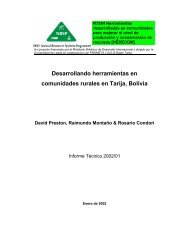
The Study Sites
Figure 2. Mutangi Dam, used for small-scale irrigation, fishing and livestock watering. In such semi-arid
regions it is a key part of the livelihood strategies (photo: Bruce Campbell)
Of particular relevance to Chivi was the forced relocation of a large swathe of
Zimbabwe’s black population in the 1950s when land policies were enforced. At this
time, land grants were being made to white soldiers who had served in WWII, and the
original inhabitants of the land were forced to move to areas like Chivi. There was
some limited redistribution in the 1980s but this did little to relieve population densities.
Even in the post-2000 period there has been negligible impact of resettlement on
population densities in Chivi (Sithole et al. 2002).
Chivi communal area covers 3534 km 2 . Its administrative centre is Chivi Business
Centre, an old settlement established in the early part of the 20th century. Chivi was
settled in the mid-19 th century (Box 1). At the start of that century the estimated
population of Chivi District was only around 15,000 (Scoones et al. 1996). By 1930 the
population had grown to an estimated 28,500, partly due to population movements
into the reserves. The southern parts of Chivi, such as Romwe, were only settled
during the 1950s, with the arrival of people displaced from farms designated for
European occupation further north. Census figures in 1962, 1969 and 1982 showed
district populations of 57 220, 80 580 and 103 656. The 1992 census shows a total
Box 1. Some historical gossip - the settling of Chivi — by Alois Mandondo and Witness Kozanayi
According to Beach (1994) the Chivi people arrived around the mid-19 th century. The ruling Mhari lineage is thought to have
come from the Mutoko area, in northern Zimbabwe, with splinters of them settling around the Mashava hills and Nyaningwe
mountains. It is reputed that the Chivi chieftaincy originated around a character called Tavengerweyi, who married among
the tribes already residing there, and had 14 sons. Some among the 14 sons rose against their ruling uncles overthrowing
them, and driving them across the Runde River into what is now called Mazvihwa communal lands. When the fleeing uncles
arrived at Runde River, the eldest refused to cross the flooded river. One of the sons pushed the resisting uncle into the
flooded river to try and drown him. The uncle managed to swim across the river and, when on the opposite bank, shouted
at the son ‘Chivi charo’ (‘sinful one’). The son retorted ‘Wazvihwa’’(‘serves you right’). Henceforth the area on the eastern
side of the Runde river was called Chivi and the western side was called Mazvihwa.’The Chivi are to this day still considered
the ‘uncles’ to the Mazvihwa.
The Mutangi people came to settle in Chivi in the early 20 th century long after the Mhari people. The Mutangi people
originated from Manicaland in eastern Zimbabwe. They came to Chivi in search of cropping land and grazing area for their
livestock. When they arrived in Chivi they settled near a mountain called Rushinga. After talking to the Mhari people, they
were allocated a new area at the foot of Mushungwi mountain. Here they had enough grazing but inadequate cropland. Again
they shifted, to Baradzanwa, where there was sufficient cropland and grazing area. Unfortunately, the stay of the Mutangi
people at Baradzanwa was short lived. There was an outbreak of a disease and the Mutangi people suspected that they were
being punished by local spirits for having settled in the area without the blessing of the spirits. They then migrated to the site
where Mutangi Dam now stands. When the dam was built in the 1940s, the Mutangi people were again relocated to their
current sites. The leader of the Mutangi people was buried behind the dam wall and the dam was named after him.
7

HOUSEHOLD LIVELIHOODS IN SEMI-ARID REGIONS
population for Chivi District of 157,428, with a growth rate of 1.98% and a population
density of 44.5 people/km 2 . Our calculated population densities for the social
catchments in 2000 were 86.1 people/km 2 for Romwe and 58.2 people/km 2 for Mutangi.
Both Romwe and Mutangi are predominantly Shona but some of the residents of
the Romwe social catchment (10%) are Ndebele who moved from Kwekwe and Shurugwi
areas in Midlands Province mainly as a result of displacement during colonial occupation
in the early 1950s. Even the Shona in Romwe came at about that time, also as a result
of displacement. This is different from Mutangi, which was settled much earlier (Box 1).
2.3 Markets, infrastructure and services
The closest large town to Romwe and Mutangi is Masvingo, the capital of Masvingo
Province, with a population of 55,000 at the time of the 1992 census. It is the major
market town in the region. The turn-off to Romwe is 86km south of Masvingo, on the
main road to South Africa, and then there is 5 km on gravel to the catchment. Other
markets for Romwe farmers are Museva and Ngundu Halt, also on the South Africa
road. Museva is a small bus stop 5 km by foot from Romwe, while Ngundu is a bustling
truck stop and local growth point 7 km by foot from Romwe or 12 km by cart or 14 km
by road. Mutangi is 6 km along a gravel road from the main sealed road running through
Chivi Business Centre. It is 80 km from Masvingo and 19 km from Chivi Business Centre.
The study areas are relatively well positioned for market access, by Chivi standards,
as Ngundu Halt and Chivi Business Centre are the two largest trading sites in the
communal area. Vegetables and other garden produce are largely traded informally at
Ngundu, Chivi Business Centre and the other smaller centres. Truck drivers stopping at
Ngundu often purchase products to take to South Africa (e.g., sweet reeds, roundnuts,
groundnuts and even maize), though the purchased amounts are small (e.g., a maximum
of a few sacks). Women and children generally walk to the points of sale, carrying
what they will try to sell on that day. There will be occasional trips, generally by bus,
as far as Masvingo, for sale of a few boxes of tomatoes or other such crops. These trips
will be timed to coincide with trips needed to purchase commodity items and farm
inputs. For the major cash crops, namely maize and cotton, there are nearby depots,
or traders come to the roads close to the study areas. Farmers speak of low prices or
high costs of transport.
The agricultural sector, particularly for commercial farmers, is relatively well
developed in Zimbabwe, with an agro-industry that supplies the full spectrum of inputs,
well-developed credit markets and suitably organised markets. The situation is not so
favourable for communal farmers. Widespread formal credit became available to
smallholders in the 1980s, but this system soon collapsed in the face of numerous
failures to service the debts. The extension system was widely expanded in the 1980s,
but by the 1990s government operating budgets had been so curtailed that extensionists
were all but absent from the field. Similar cutbacks have occurred with the veterinary
service. In many years Chivi farmers received free inputs (seed and fertiliser) as part
of drought relief efforts, but by the late 1990s such schemes were no longer possible
for a government increasingly facing economic problems. Soon after independence,
agriculture was stimulated by the expansion of centralised marketing systems, which
meant that remote rural producers received subsidised transport of their crops, but by
the mid-1990s marketing had been liberalised and subsidies withdrawn. Withdrawal of
subsidies also has occurred in non-agricultural sectors, and now payments are required
for senior schools and health clinics. Withdrawal of subsidies for agro-industry has
seen a rise in fertiliser prices.
2.4 Climate, agricultural potential, land use and risk
Long-term mean annual rainfall at Chivi Business Centre is 545 mm (1913-2001). The
rainfall average in Romwe is estimated to be 620 mm, while that in Mutangi is 550 mm
— Romwe thus has higher potential for dryland production. On average, 89% of the
8

The Study Sites
annual rainfall at Chivi Business Centre is received during the summer rainy season
from November to March. However, rainfall amount, intensity and distribution are
highly variable, and inter-annual variation is large (Figure 3). The long-term mean has
a standard deviation of 207 mm or coefficient of variation of 38%. Droughts are recurrent
in the region, and the most recent in 1991/92 was the worst on record, when only 83
mm of rain fell in the Romwe catchment. Throughout the country there was almost
total crop failure, and livestock populations plummeted. Researchers can identify wet
and dry rainfall cycles (Moriarty and Lovell 1998), with, for example, the 1970s and
late 1990s having above-average rainfall, while the 1980s precipitation was below
average. The questionnaire survey captured dryland crop production for the 1998/99
season, a period with 15% above-average rainfall at Chivi Business Centre — a high
rainfall year during a wet period. Masvingo is the closest site for which long-duration
temperature and evaporation records exist. Monthly average daily maximum
temperatures vary between 22 o C in June and 29 o C in October. Average minimum
temperatures range between 5 o C in July and 17 o C in January.
Figure 3. Annual rainfall at Chivi Business Centre
1400
1200
1000
Annual rainfall (mm)
800
600
400
200
0
1913 1923 1933 1943 1953 1963 1973 1983 1993
Year
Communal lands make up 49% of Zimbabwe. Approximately 75% of these lie within
natural regions IV and V which are characterised as being unsuitable for intensive
farming due to low and variable rainfall, and poor soils. Most of Chivi, including Mutangi,
falls within natural region IV, but a central area of hills is more typical of natural
region III (characterised as being wetter and more suitable for farming), and it is in
this area that Romwe is situated.
In the Romwe area the valley floors, at about 700 metres above sea level (m.a.s.l.),
are encircled by relatively steep rocky hills, with summits of about 1000 m.a.s.l. Mutangi
is less hilly, with altitudes between 850 m.a.s.l and 950 m.a.s.l. Both areas are
underlined by Precambrian gneiss with occasional dolerite intrusions. The former gives
rise to nutrient-poor soils, while the latter produces more fertile soils. In Mutangi
there are sodic soils in the low-lying areas near the drainage lines, making up 36% of
the physical catchment (Gotosa et al. 1999). These soils are not cultivated and are
easily eroded.
9

HOUSEHOLD LIVELIHOODS IN SEMI-ARID REGIONS
Land use is typical for communal areas in this region, with rainfed cultivation and
rough grazing dominating the landscape. In Romwe the rainfed cultivation is on the valley
floors with grazing in the densely wooded miombo woodland in the hills (Figure 4). In
Mutangi the landscape is gently undulating; the few hills have some grazing and degraded
woodland, but more important for grazing are the areas covered by degraded mopane
woodland on sodic soils along the water courses (Figure 5). Households also have small
garden plots either close to their homestead and fed by wells or near key water points.
Figure 4. The view south-east from the top of the Romwe inselberg (photo:
Patrick Moriarty)
Figure 5. Gently rolling landscape in Mutangi showing areas cleared of woodland
for dryland crops and strips of Colophospermum mopane in the low-lying areas
along streams (photo: Martin Hodnett)
10

The Study Sites
Risk and uncertainty are endemic to such dryland farming systems (Scoones et al.
1996). Rainfall is the key resource in semi-arid rainfed agriculture. Thus when the
rains arrive, how much rain falls, how it is distributed within the season and when the
season ends are critical to the production achieved. The nature of a season is
unpredictable, but more often than not rainfall is insufficient or poorly timed. Studies
at Romwe have found that too much rain can do as much damage as too little, and
when the rain arrives can be as important as how much falls (Moriarty and Lovell
1998). Crop failure in the Romwe catchment, on the gneissic soils, is as likely to follow
from waterlogging due to too much rain as from drought. Rainfall is not the only
component of risk and uncertainty; others include fluctuations in input and commodity
prices, pest and disease outbreaks (for humans, livestock or crops), and the condition
of the country’s macro-economy (which determines, among other things, levels of
remittances and availability of non-farm employment). In an area where off-farm
work and remittances are often critical, a sudden decrease in employment can have as
devastating an effect on livelihoods as a drought or flood.
Our data are generally presented for four quarters of the year, corresponding to
the enumerating schedule. During quarter 1 (March to May 1999) at the start of the dry
season, rainfed crops were being harvested and, where possible, marketed. During
quarter 2 (June to August 1999) people turned to irrigated production in small garden
plots and other non-farm activities (brick moulding, building, thatching and various
woodland-related activities). In the third quarter (September to November 1999) dryland
fields were being prepared for planting and the irrigated gardens were maintained.
The fourth quarter (December 1999- to February 2000) was the height of the growing
season for the rainfed crops.
2.5 Institutional framework
During the colonial period, legislative controls on woodland use were established,
starting with the Native Reserve Forest Produce Act in 1928, and subsequently the
Natural Resources Act (1942) and the Forest Act (1948). These Acts increased State
control over natural resources (largely woodland resources), especially in the communal
lands. Traditional leaders, together with government extension agents, were responsible
for enforcing rules governing woodland use in the communal lands. The traditional
authority was also responsible for tax collection and overseeing other administrative
responsibilities. The traditional structure consists of a hierarchy of chiefs, headmen
and, at the local level, sabhukus (kraalheads).
At independence one of the first major policy initiatives was to change the
governance structure for communal areas, with consequent changes to natural resource
institutions (Mandondo 2001). Through the District Councils Act (1980), the Communal
Areas Act (1982) and the 1984 Prime Minister’s Directive on Decentralization, the power
to allocate land was removed from traditional chiefs and headmen and given to the
District Councils. In addition, local organisations known as the Village Development
Committees (VIDCOs) and Ward Development Committees (WADCOs) were established.
These formed a parallel institution to the traditional authority already in place at
village level. WADCOs and VIDCOs are elected bodies and have the responsibility to
spearhead development in areas under their jurisdiction as well as monitor natural
resource use and land allocation. These new administrative structures further stripped
traditional authorities of their powers. In 1998 the government revised the position of
the WADCOs and VIDCOs, having seen that they were ineffectual. This has restored
some of the authority of the chiefs through the enactment of the Chiefs and Traditional
Leaders Act (1998). However, the legislation now supports two power structures, the
traditional structures and the VIDCO/WADCOs, without clarifying the various roles and
responsibility. It should be noted that even when such powers as land allocation were
withdrawn, the traditional authority continued to exert an influence, albeit with less
absolute powers than before.
11

HOUSEHOLD LIVELIHOODS IN SEMI-ARID REGIONS
Decentralisation is now high on the agenda of the State, inspired in part by the
appeal of an international’‘back to the people’ option that is a potentially more ethical
and effective alternative to centrally directed management of natural resources
(Mandondo 2001). Of late a new rural development thrust, coming with structural
adjustment programmes, has also encouraged cash-strapped governments in many
African countries to decentralise by passing on some roles to lower levels of government.
In spite of the envisioned merits of decentralised natural resource management,
experience in Zimbabwe generally suggests that the State is reluctant to relinquish
power and control. The State view of appropriate management of resources still appears
to extend to local communities through a centrally directed structure and process.
Effective control is still largely vested in the State or bureaucracies under its direction
like the Rural District Councils. State regulation is, however, severely undermined by
its inherent incapacity to assert effective control.
The communal lands are officially State land but managed by a combination of
modern and customary law. Considerable responsibility now resides at the district
level, where the Rural District Council is able to mobilise limited funds for development
activities and provides the legal framework for resource management (through bylaws)
(Mandondo 2001). People in the study area complain that they have minimal
interaction with the district officials, and it is blatantly obvious that the by-laws have
almost no function in the village settings. The de facto rules and regulations operating
at the village level are centred on the traditional authorities (Mandondo et al. 2002;
Nemarundwe 2002c).
2.6 The national economy
Like other post-independence African countries, Zimbabwe has been implementing
various macro-economic policies in an attempt to improve the welfare of its people.
Two diametrically opposite policy regimes were implemented in the first two decades
of independence. In the 1980s fiscally driven redistribution, import substitution and
government controls were adopted, while in the 1990s emphasis was on getting prices
right, through structural adjustment programmes. Neither yielded the desired outcomes.
The period immediately after independence in 1980 saw major improvements of social
services, such as health, education and infrastructure. Agriculture also performed
very well in the first half of the 1980s (Rukuni and Eicher 1994). However, in the
second half of the decade, the economy declined, forcing the government to adopt (in
1991) an Economic Structural Adjustment Programme (ESAP), designed with assistance
from the World Bank and the International Monetary Fund (Addison 1996; World Bank
1996).
While the reform programme may have had a series of positive impacts on the
large-scale commercial farming and manufacturing sectors (Addison 1996; World Bank
1996), a central question is whether the programme, as implemented in Zimbabwe,
has had positive or negative impacts on the rural smallholder sector. The first half of
the 1990s was marked by decreasing subsidies for farming inputs and social services,
increasing unemployment, declining real wage levels and, presumably, decreasing
remittances (World Bank 1996; Oni 1997). Most African countries introduced
liberalisation measures, in response to both internal and external crises resulting from
increases in the price of petroleum, adverse commodity terms of trade, wars and
political upheavals, droughts, wrong domestic policies of overvalued exchange rates,
subsidised imports and distorted factor market prices, overextended and inefficient
public sectors, and poor bureaucracies (Wangwe and Musonda 1998). The ESAPs were
intended, but largely failed, to integrate the African economies into the global economy,
since adjustment measures such as trade liberalisation help open up economies and at
the same time expose domestic industries to external competition. Debate about the
social and distributional impact of reforms has accompanied economic reform
programmes from their inception. For example Ahmed and Lipton (1997), in reviewing
the literature on the impact of structural adjustment on sustainability of rural
12

The Study Sites
livelihoods, conclude that there is no systematic improvement or decline in rural
livelihoods as a result of adjustment measures.
In the late 1990s and into the 21 st century the economy declined even further,
when drastic moves were taken by government to win the votes of the populace in the
face of declining popular support and the threat of election defeat. In addition, the
large expenses committed to the civil war in Congo stretched the national coffers.
This period saw massive inflation (57% in 1999, 60% in 2000, rising to over 100% by
2001), collapse of many industries, including the tourist industry, rapid rise in
unemployment, subsequent massive movement of young able-bodied men to South
Africa (especially from late 2001) and breakdown in law and order. Our quantitative
survey data comes from March 1999-February 2000, so we largely missed the major
meltdown in the economy, but the qualitative data continued to the end of 2001.
The average annual growth in real GDP between 1979/80 and 1998/99 was just
under 2.2%. Growth rates of more than 7% per annum were achieved only in 1979/80
(10.7%), 1980/81 (9.7%), 1984/85 (7.6%), 1987/88 (7.3%), 1993/94 (7.8%) and 1995/96
(8.5%). In most cases, these apparently impressive growth rates merely reflected low
GDP in the preceding year due to factors such as drought. At the time of our quantitative
survey the GDP growth was 0.1% in 1999, 4.9% in 2000, and a further such decline was
expected in 2001.
2.7 Why Chivi and why two case-study sites
The research on livelihoods was conducted within the framework of a much larger
research project on micro-catchments and common property resources. The Institute
of Environmental Studies (University of Zimbabwe) led the work, in close collaboration
with the Department of Research and Specialist Services (Zimbabwe Ministry of
Agriculture), Centre for Ecology and Hydrology (UK) and the Center for International
Forestry Research. CARE led development work in both catchments, as part of a much
larger development project throughout Masvingo Province, in which small dams were
rehabilitated, irrigation was introduced or improved, and organisations were facilitated
to provide local management.
In many parts of the world there are vast shields of igneous and metamorphic
rocks. The most common of these ‘hard rocks’ are granites and gneisses. Large parts
of this geological type lie in least-developed, semi-arid regions. This is especially true
in parts of Brazil, peninsular India, Sri Lanka, Korea, China, the Red Sea region, West
Africa and much of central, eastern and southern Africa (Lovell et al. 2002). Chivi is
relatively typical, from a biophysical perspective, of this vast domain (Lovell et al.
2002). Within Zimbabwe, Chivi is similar to large portions of the communal areas
running from the north-west, down the central and eastern areas to the south of the
country.
Rather covering many locations in Zimbabwe (and beyond) we decided to focus
our work, providing the opportunity for in-depth understanding through frequent returns
to the same households and living at the study sites. We selected two sites to provide
some degree of contrast, while choosing nearby sites for logistical reasons. Romwe
was selected as it had a history of relevant research, while Mutangi was a contrasting
site with greater levels of land degradation, lower rainfall and, possibly, a poorer
community. We hypothesised that in Mutangi, with its harsher conditions than Romwe,
there would be less intensification of land use and there would be greater poverty;
thus allowing us some insights into household variability in relation to site differences.
While being empirically based we have attempted to focus on processes of relevance
to semi-arid regions elsewhere in Zimbabwe and beyond. From the specific
characteristics of Romwe and Mutangi, relating to site and history, we have attempted
to derive principles relevant to policy in semi-arid regions generally. Instead of engaging
in the development rhetoric based on generalisations, we enter the debate from an
attempt to understand the intricacies of everyday life.
13

Methods
3. Methods
3.1 Livelihood questionnaire data collection
In order to collect data to support the livelihood analysis, a household questionnaire
was designed and administered. The survey paid particular attention to the need to
ask questions that did not require long–term, detailed memory, and were therefore
answerable with a high degree of accuracy. Therefore, highly disaggregated data were
collected, and then aggregated by the analysts. The uniqueness of the survey has to
be noted. The survey followed the methods of Cavendish (1999a; 2002a), with some
modifications that we believe are improvements. Cavendish (1999a) notes that such
survey instruments lead to unique empirical results; very few of the resource-use
patterns recorded would be captured in standard household budget surveys (e.g.,
collection of wild fruits, collection of poles). Standard surveys consistently
underestimate woodland-based income; hence overestimating agriculturally based
income. Cavendish (1999a) paid particular attention to design recall periods to capture
the use of products that is seasonal, casual and small. For some variables we recorded
both three-monthly and weekly recall data. The three-monthly recall results proved
to return much lower estimates than those based on one-week recall. As many of our
results are based on the shorter recall periods, we believe we have achieved greater
accuracy. Particular differences to the methods of Cavendish (2002a) were the attention
to labour (he collected no labour data) and our collection of data on goods and services
derived from livestock (he only collected numbers of animals and cash sales). The
price of detail in a questionnaire, with up to 24 visits per year to sampled households,
is respondent fatigue and very time-consuming data capture and analysis. The household
survey was designed to be completed in less than one hour at a household during the
first round of each quarter. The subsequent six rounds in a quarter were quicker (often
less than half an hour). Nonetheless, halfway through the survey it was judged that
households needed to be compensated for participation in the survey, and households
subsequently received a small gift of appreciation per quarter (a packet of kapenta
dried fish valued at Z$65). Despite more or less fulltime attention to data entry, cleaning
and analysis, some of the more complicated modelling is only now being undertaken,
more than two years after the final data were collected (Moyo, forthcoming; Zindi,
forthcoming). One limitation of this work is that we pay scant attention to intrahousehold
decisions and allocation patterns.
3.1.1 The field survey and the recall periods
The survey was conducted as a quarterly household income and expenditure survey,
over 15 months from late 1998 to early 2000 (Table 1). The focus of the survey was on
tracking how households use their available resources in the pursuit of livelihoods, and
the returns that they receive from these activities. Because of the seasonal variability
facing these villages, data were collected quarterly. The first visit (round) in each
14

quarter was structured around major activities for which households could reasonably
be expected to remember over three-month periods. The subsequent five visits (rounds
2-6) in a quarter collected information from short recall questions — for example,
obtaining estimates of labour inputs for the previous 24 hours, thereby providing five
days of labour data per household per quarter.
The nomenclature used in Table 1 for quarters and rounds is somewhat confusing
when it comes to reconstructing a year of data. ‘Quarter 1, Round 1’ and ‘Quarter 1,
Rounds 2-6’ represent the field schedule for enumerators. In ‘Quarter 1’ the three-
Table 1. Household survey structure
Survey
segments
Date
conducted
Dates covered
Type of Data Collected
Quarter 1
Round 1 March 1999 Starting conditions; monthly
.
Background information on the household (shelter, land size,
activities from Dec. 98 to demography);
Feb. 99; weekly activities for Three monthly recall on large items, including remittances,
a week in March 99
.
salaries, wages, dryland crop production, major input costs,
livestock dynamics, wood use patterns.
Weekly recall on other items (smaller items that are not easily
remembered over a month), including garden production,
.
livestock production (milk, draft etc.).
Water use (not quarter specific)
Rounds 2-6 March to March to April 99
Weekly recall questions covering woodland harvesting, purchases
of inputs, income sources for a male, female and child in
April 1999
.
the household
Daily recall for labour (i.e. what was done the previous day), for
a male, female and child in the household
.
Quarter 2
Round 1 June 1999 Monthly activities from March Same items as for Quarter 1, Round 1, but excluding
to May 99; weekly activities the background info that was relatively constant
for a week in June 99
.
Quarterly water use patterns
Rounds 2-6 June to June to July 99 Same items as for Quarter 1, Rounds 2-6
July 1999
.
Quarter 3
Round 1 Sept. 99 Monthly activities from June Same items as for Quarter 2, Round 1
to Aug. 99; weekly activities
for a week in Sept. 99
.
Rounds 2-6 Sept. to Sept. to Oct. 99
Same items as for Quarter 1, Rounds 2-6
Oct. 99
Quarter 4
Round 1 Dec. 99 Monthly activities from Sept.
to Nov. 99; weekly activities
for a week in Dec.
Rounds 2-6
Quarter 5
Round 1
Dec. 99 to
Feb. 2000
April – May
2000 for
Mutangi, and
April to July
2000 for
Romwe
Dec. 99 to Feb. 2000
Monthly activities from Dec
99 to Feb 2000; weekly
recall for the time when the
survey was done.
. Same
. Same
items as for Quarter 2, Round 1
items as for Quarter 1, Rounds 2-6
.
.
Covered the same items as for Quarter 2,
Round 1.
Additional background information for
households (e.g. village name, organisations
involved in, access to collective gardens)
15

HOUSEHOLD LIVELIHOODS IN SEMI-ARID REGIONS
month recall covers the period December to February, but the weekly and daily recall
questions (Rounds 2-6) cover weeks and days during the time of the surveys (i.e., in
March and April; see Table 2). In reconstructing a year of income and expenditure, the
weekly and daily recall questions from Quarter 1 rounds are to be matched with the
three-month recall questions for Quarter 2 Round 1. Thus the first quarter for which we
have a full set of data on all questions is March to May 1999. This necessary overlap
created the need to conduct a ‘5 th Quarter, Round 1’. The above overlaps meant that
some data were not used when constructing annual budgets. However, the data were
not completely discarded in that they were used for specific purposes and/or for checking
consistency of results.
Table 2. Reconstruction of quarterly data
Survey
instruments (see
Table 1)
Date collected in the
field
Three monthly recall
variables used for:
Weekly and daily recall
used for:
Q1R1 March 1999 Mar-May (Quarter 1)
Q1R2-6 Mar-May Mar-May (Quarter 1)
Q2R1 Jun Mar-May (Quarter 1) June-Aug (Quarter 2)
Q2R2-6 Jun-Aug June-Aug (Quarter 2)
Q3R1 Sept June-Aug (Quarter 2) Sept-Nov (Quarter 3)
Q3R2-6 Sept-Nov Sept-Nov (Quarter 3)
Q4R1 Dec Sept-Nov (Quarter 3) Dec-Feb (Quarter 4)
Q4R2-6 Dec-Feb Dec-Feb (Quarter 4)
Q5R1
Apr-May 2000 Dec-Feb (Quarter 4)
–
–
–
–
–
–
Table 3. Original sample of households in Romwe and Mutangi villages
Village name Number of households
sampled
Village name
Number of households
sampled
Romwe
Mutangi
Chikanda 22 Chimuti/Zivengwa 7
Dhobhani 10 Ngindi/Mubviigwi 4
Sihambe 11 Venganai/Murazvo 2
Matenhese 8 Hlanga 16
Tamwa 17 Masimba 4
Ndabaningi 22 Chidanhika/Vurayayi 5
Munikwa 6 Mafuka 3
Puche 17 Matangani 4
Joni 8 Madamba/Tapera 2
Magomo 4 Tambu 9
Gwarisa 9
Tichagwa 6
Hwari 11
Mudzingwa 11
Manikayi 4
Chimwa/Njini Zivanai 11
Mutangi 12
Pedzisai 0
Total 245
16

Methods
Weekly recall is important for collecting accurate data but one needs a large
number of such recall events in any single year. We had 20 rounds of weekly recall data
for the year of the study for most variables, but we did have a problem with livestock
(for draft, transport and milk) and gardening. The weekly data for these activities was
collected in Round 1 with the other agricultural data, and so was only done four times
per year. This was particularly a problem for draft, which is used at a very specific
period of the year and then only for a short time. As the weekly data for the December
to February quarter covered the period of high use in December, we assumed our
weekly recall was an appropriate figure for that month but for the other two months in
the quarter we assumed they were the same as the average for the next quarter.
3.1.2 The sample
The Romwe area contained 417 households in 10 villages, with three of the villages
falling, at least partially, in the physical catchment of the Chidiso collector well (Tamwa,
Dobhani and Sihambe). The Mutangi area contained 453 households in 18 villages, with
at least five villages being partially or completely in the physical catchment of the
Mutangi Dam. A complete household list was compiled for the villages and a stratified
random sample was taken with households selected from each of the villages in
proportion to the total household number in a village (Table 3). In Mutangi one of the
18 villages in the area (Pedzisai) was not in the original village and household listing
for the catchment, resulting in Pedzisai households not being sampled. The distribution
of households within the villages is shown in Figure 23 and Figure 28.
The target sample size was 125 households each from Romwe and Mutangi. Contact
was made with 245 households in total in the first round of the questionnaire. Because
of enumerator problems in the third quarter in Mutangi, a number of cases had to be
deleted from the final data compilation. Thus the final data matrix has 124 households
in Romwe and 75 in Mutangi (total 199). For a number of analyses it was possible to use
the full data set when annual statistics did not need to be compiled from third-quarter
data.
3.1.3 Enumerators and supervisors
Ten enumerators were selected from applicant pools of young adults in each area. The
enumerators were trained over a week-long intensive session that included numerous
pre-tests of the questionnaire. The enumerators were trained to administer the
interviews in English and in Shona, the local language. Each enumerator was assigned
approximately 25 households that were contacted repeatedly as described above.
Supervision took place at a number of levels. The research assistants based at the
study sites made random checks and weekly follow up on enumerators. Post-fieldwork
coding was conducted in Harare, during which errors and contradictory answers were
identified. Questionnaires with problems were returned to the field supervisors and
enumerators for clarification (and in many cases enumerators had to return to the
interviewed household).
3.1.4 Units of goods and services used
To obtain physical measures of production, locally meaningful units were used (e.g.,
contours to define area, wheelbarrows and carts for amounts of manure). Measurement
units that are commonly used by communal households are sometimes not ‘standard’
units. However, to ensure a common standard by the participants, these locally
understood units were used, most of which are based on volume. To assist conversion
a separate survey was conducted in which local units were measured in terms of standard
units (e.g., kilograms, acres; see Appendix 1).
17

HOUSEHOLD LIVELIHOODS IN SEMI-ARID REGIONS
3.1.5 Surveyed prices
Prices were collected in the household surveys in cases where goods and services were
bought and/or sold. Where possible, we have used 5% trimmed means for prices. A
trimmed mean is the arithmetic mean calculated after the highest 5% and lowest 5% of
cases have been eliminated. Eliminating the extreme cases from the computation of
the mean results in a better estimate of central tendency, especially when the data
are non-normal (SPSS Version 10). The non-trimmed mean sale price is used in cases
with few observations for prices, such that the 5% trimmed mean cannot be computed.
In all cases the standard deviations reported are for non-trimmed means. Prices are
vary widely across and within years for some goods and services (e.g., Scoones et al.
1996), making calculations sensitive to the price variable. For maize, we used two
prices: one for dryland maize and the other for garden maize, as each is generally
produced at different times of the year, with widely different products and prices
(green maize sold from gardens at roadside markets, while dryland maize is sold as
less valuable dry maize). Our approach of using a single price across all households
probably means that we have reduced the difference between the poor and the rich.
Our key informant interviews indicate that the rich hold products (e.g., grain and
livestock) until prices are better, both because they have better access to market
information (e.g., relatives working in urban areas) and because they have the resources
not to make frequent crisis sales. Turner and Williams (2002) document similar
phenomena in West African livestock markets in semi-arid regions.
All prices were captured in Zimbabwe dollars, for which the exchange rate
conversion was Z$38-40 to US$1 during the time of the survey (Appendix 2). Values
reported are all in 1999 Zimbabwean dollars.
3.2 Livelihood questionnaire data analysis
3.2.1 The sectors for analysis
In analysing household livelihoods, we identify seven classes of activities that are
subsequently referred to as sectors (Table 4). For some analyses, we subdivide the
Domestic sector into sub-sectors of Leisure and sleep, Academic and Basic (i.e., any
other domestic activity).
Table 4. Sectors and activities for analysis of household livelihoods
Sector
Dryland crops
Gardening
Livestock production
Woodland use
Domestic
Wage labour and home industry
Remittances and gifts
Activities/products
Maize, sorghum, millet, groundnuts, etc. (rainfed)
Tomatoes, green beans, okra, etc. (irrigated)
Cattle, donkeys, goats, pigs, poultry etc.
Wood and non-wood products including construction wood, fuelwood,
thatch, small animals, fruits, mushrooms, etc.
Maintenance of basic household health and nutrition including: preparing
and eating meals, housekeeping and construction, attending gatherings,
travelling, leisure and sleeping, and education
Wages from local employment (e.g. domestic and agricultural work) and
cash- generating home industries such as carving, brick moulding, fixing
bicycle/implements, making household utensils from scrap metal, etc.
Cash sent by family members not living with the household, and gifts
18

Methods
Cash expenses and income were tracked for all sectors with a number of questions,
some of which overlapped to allow crosschecking. For dryland crops, there was a
record of sales of production by crop, using quarterly recall. For the smaller and more
continuous production of garden crops, weekly recall data was collected by crop.
Quarterly recall was used for large woodland items for construction, but weekly recall
also captured this in addition to firewood and the various non-timber forest products.
Expenses for large domestic purchases (e.g., school fees) were based on quarterly
recall, as were data for remittances and wages. In addition to the above records, data
were collected, using weekly recall, for all cash received and expended by source.
This was subsequently classified into sectors.
In a number of cases, it was not possible to separate dryland crops from gardening
in terms of cash expenses (e.g., fertiliser was purchased and subsequently allocated
to different crops but it was not possible for some respondents to accurately apportion
the inputs amongst crops for each type of agriculture), time allocated (e.g., marketing
of products from both types of agriculture at the same time), or income (i.e., income
from both types of agriculture was reported together). Accordingly, we have allocated
all ‘Agriculture General’ into dryland crops and gardening according to the proportions
(Table 5) based on the data that did apportion amounts between dryland crops and
gardening. We feel that this procedure is justified as the cases of ‘Agriculture General’
were less frequent than the cases when agriculture was specifically allocated.
Table 5. Proportions used to allocate ‘Agriculture General’ between dryland crop production and gardening
Dryland crops as a proportion of dryland crops
plus gardening (averaged over all households)
Expenses (quarterly recall data, for items requiring large
cash expense) 0.92
Expenses (weekly data) Child 0.05*
Female adult 0.75
Male adult 0.76
Time
Income (weekly data)
Child
Female adult
Male adult
Done on a household by household basis using the proportion
of time allocated specifically to dryland and gardening
0.45
0.58
0.75
* This would mean that 5% of the child expense figure is allocated to dryland crops with the remaining 95% allocated to gardening
3.2.2 ‘Income’ terminology and the calculation of net income
We use the term income to cover cash income and subsistence (or in-kind) income. We
recognise gross and net income. Gross income is the full amount of income without
any subtraction of expenses. Net income is exclusive of all cash and in-kind inputs,
excluding labour, following the approach of Cavendish (2002a). The exclusion of labour
from the measure is the usual approach in rural household studies (Ellis 2000). Gross
income was calculated on a sector basis from the stated production figures (e.g., milk
consumed and milk sold, manure used and sold, poles used and sold, etc.) and the
stated prices. Net income was less expenses recorded in the weekly recall data. A
proportion of the expenses was allocated to cash income and the remaining amount to
subsistence income, in proportion to the ratio of gross cash income to gross subsistence
income for the sector in question. We use the word ‘total’ to indicate the sum of cash
and subsistence income. The concept of net income, as employed here, is a standard
measure of welfare, used in most rural income and expenditure surveys. While
19

HOUSEHOLD LIVELIHOODS IN SEMI-ARID REGIONS
consumption is often preferred to income as a welfare measure in household studies
(Deaton 1980), in this and other rural studies in Africa the distinction between net
income and consumption is not great. This is because some quantitatively economic
activities represent both consumption and income (e.g., the consumption of ownproduced
goods and own-collected woodland products) (Cavendish 1999a). The total
gross income is normally compiled from the many components of income within a
sector (e.g., livestock income is the sum of income from manure, draft power, milk,
transport, etc.). We present gross income data instead of net income (the standard
measure) because it would have been extraordinarily difficult to find the expenses for
each sub-component (e.g., for livestock, the veterinary costs and all the other costs
would have to be apportioned by the components).
3.2.3 Statistical analysis
For the simple case of comparing variation in continuous variables across single factors,
one-way ANOVA was used to determine whether differences existed among the means.
If a significant difference was found at the 5% level, pair-wise multiple comparison
tests were conducted. Multiple comparison tests describe confidence levels for an
entire system of intervals, simultaneously, for a given variable. For example, in Table 8,
for the variable adult males, there is a system of four confidence intervals, one for
each wealth quartile. Several types of multiple comparison tests are available, the
appropriate use of which depends on whether variances of the populations are equal.
Levene’s homogeneity-of-variance test was implemented to test for equality. The
Scheffe pairwise test is applied to cases depicting homogeneous variance and the
Dunnett C test is applied to cases depicting non-homogeneous variance. For those
readers wanting to see standard deviations for all the means that are presented in
tables and figures in this document, we have compiled these on the project CD-Rom
(Sampurna et al. 2002) available from the authors.
Where we analyse differences amongst quarters, we have a repeated measures
design, as the dependent variable is measured on the same case. In much of our
analysis, ‘quarters’ is only one of three independent variables, the others being ‘wealth
quartile’ and’‘site’. Differences due to these variables and interactions among variables
were investigated with a single analysis of variance, using the general linear model
procedure for repeated measures (the repeated measure being the quarter). In these
cases the significance levels for a single analysis are presented across several tables
for the different means being compared. For instance, for the single analysis of cash
expenses incurred for dryland crops, the statistical results are presented in the first
line of Table 19 (effect of quarters), Table 20 (effect of wealth quartile) and Table 21
(effect of site).
We used the gross cash and subsistence income data for the different sectors to
classify the households into different types (Section 7). This involved using a multivariate
cluster analysis technique, with the similarity between each and every household
calculated on the basis of squared Euclidean distance and the households clustered
into groups using average linkage clustering. In this way we were able to recognise 10
different types of households, each type with their characteristic set of income sources.
The similarities among the different types were explored using principal component
analysis with the data in the analysis being the mean gross income levels for each of
the sectors.
We have also examined the variation in total net income and net income for
different sectors in relation to a variety of socio-economic variables (e.g., age of head
of household) by using analysis of covariance, which allows the use of categorical and
continuous independent variables (Section 8.3). Where we want to determine what
variables relate to the presence or absence of a condition (e.g., being above or below
the food poverty line) we have used stepwise binary logistical regression.
All analyses were conducted with SPSS Version 9 or 10. The raw data, various
intermediate data files and the command files (all in SPSS format) are stored on the
20

Methods
project CD (Sampurna et al. 2002). Two files on the CD describe the survey, one giving
further details of procedures in data collection and another providing a guide to the
SPSS command files.
3.3 Participatory rural appraisal (PRA), participatory observation
and action research
Various participatory tools and techniques were used during the study period. The first
major PRA exercises were conducted in late 1998, but throughout the life of the project
numerous meetings were held, many of them using PRA tools. A number of key informant
interviews were conducted to capture the diversity of and changes in livelihood
strategies. Some of these are presented in the boxes of this book as cases studies of
households (for others see Nemarundwe 2002b; Sayer and Campbell 2002; Sithole et
al. 2002). Names of individuals have been altered to maintain confidentiality. In three
villages in Romwe, short key informant interviews were conducted with all households
to explore the patterns of human mortality in the last few years. From early 1999 to
late 2001 one research assistant was based in each of the two villages, so participant
observation was extensive and written up in various field and monthly reports. During
this period the researchers were accepted as part of the community, especially in
Romwe, and participated in all aspects of community life. In addition, a researcher
working on the livelihood data was based in Romwe catchment for one year (1999/
2000), at the time of the livelihood survey. The participatory tools, the participatory
observation and some components of the action research are described in detail in
Nemarundwe et al. (1998), Nemarundwe (2002a,b,c) and Nemarundwe and Kozanayi
(2002).
Action research mainly covered irrigation development, garden expansion, soil
and water conservation, micro-credit, tree planting and capacity building of local
organisations. Previous research in the area as well as extensive consultation with the
community ruled out some lines of action research (e.g., anything relating to livestock
or fuelwood; Campbell et al. 1997b, 2000a). The action research allowed fieldworkers
to be part of real-world allocation decisions. In this action research we were greatly
facilitated by CARE, who was implementing a large development project in the area,
based on small-dam rehabilitation, while focussing on the sustainable livelihood
approach.
3.4 Biophysical resource surveys and the geographical information
system
A number of biophysical surveys were conducted, allowing the following data layers in
the GIS: land cover, vegetation types, cropping patterns (in a subset of the area),
geology, soils, household locations and water sources, as well as the usual physiographic
features. We were able to overlay income and other household characteristics on the
biophysical data.
3.5 Systems modelling
While it is ideal to collect longitudinal data from households, this is often not possible
in the time frame of a single project. We therefore used a systems model to investigate
likely impacts of development options on livelihoods (Chapter 10). A systems model
was also produced as a means to integrate different components of the project and to
integrate the different capital assets and multiple livelihood strategies).
The model development and the actual model are described in detail in Cain
et al. (2001). Here we give a brief overview. The model was based on a Bayesian
Network (BN), which consists of three elements:
21

Methods
• A set of nodes representing management system variables, each with a finite
set of mutually exclusive states.
• A set of links representing causal relationships amongst these nodes.
• A set of probabilities, one for each node, specifying the belief that a node will
be in a particular state given the states of those nodes that affect it directly
(its parents). These are called conditional probability tables and can be used
to express how the relationships amongst the nodes operate.
A fully functioning BN is a compact representation of the joint probability
distribution over all the variables in the network. Therefore, the impact of entering
findings about one of the variables can be observed as it affects the marginal
probabilities of the other variables in the network. The software used in this study is
called Netica and is produced by the Norsys Software Corporation (www.norsys.com).
Three workshops were held over a period of two years (two of these also had agenda
items other than modelling). At the first, representatives of all stakeholders in the
project were asked to list all the things that affected rural livelihoods in the two
catchments and to describe the relationships between them. However, as the resulting
collection of variables and relationships would have resulted in an extraordinarily
complex model, it was used as the starting point from which key variables could be
selected, at the second workshop. Subsequently, a prototype model was developed by
Jeremy Cain using Bayesian Networks and distributed to the research team for comment
and use. The first model was used to explore the impacts of micro-credit interventions
(see descriptions of some aspects in Campbell et al. 2001a and Sayer and Campbell
2002). On the basis of feedback, a relatively advanced BN diagram was developed and
brought to the third four-day workshop, attended by seven researchers in different
fields (Jeremy Cain: modeller; Peter Frost: ecologist; Manyewu Mutamba: microeconomist;
Alois Mandondo: sociologist; Francis Mugabe: agricultural scientist; Chris
Lovell: hydrologist; Bruce Campbell: natural resource scientist) as well as the two
research assistants living in the study sites (Witness Kozanayi and Osiman Mabhachi).
The team members were then encouraged to change and extend the BN until it met
their needs. This model was built to explore our understanding of the best ways too
improve the cash income of poor people, as this was considered to be the key to other
livelihoods improvements. We also examined ‘vulnerability’, which is an amalgam of
levels of cash income and the resilience of that income. The focus on cash income was
partly practical (to simplify) and partly the recognition that cash income is a crucial
component of broader livelihood needs (Sections 6.5.1 and 6.5.4).
Once a final model structure had been agreed, the project team specified the
functionality of the model by completing the conditional probability tables. This was
done primarily using the results of the livelihood questionnaire survey, but other field
results were used for specific parts of the model. Where the surveys were unable to
provide the necessary information, the expert judgement of the team was used, so
some relationships were specified on the basis of limited data. With the model complete,
the project team carried out a preliminary exploration of the model operation by
changing the value of certain variables in the network and examining how other variables
responded to this. Where unexpected results were found, the reasons were identified
and either accepted as genuine or corrected as errors. A sensitivity analysis was then
performed on the model to identify the variables in the system that control peoples’
livelihoods most strongly. The results of the sensitivity analysis were presented to the
team. Once again, where surprising results were found, the research team used the BN
to explore how these results had arisen. In this way, both the model outputs (in the
form of the sensitivity analysis) and the model operation were used to improve the
research team’s understanding of livelihoods in Romwe and how resource management
strategies might enhance them.
Model building was thus an iterative process; it provided insights that changed
the way the project was being implemented and, with a deepening understanding
gained from various aspects of fieldwork and data analysis, the model was improved.
22

4. The wealth index and its variation
In conducting the analyses in this paper, we were interested in how income sources differ
amongst households. While we return to the topic of differentiation in detail in Chapters 7
and 8 , here we need to introduce one of the major differentiating factors: asset status, as
this will be used in the descriptive results presented in the subsequent sections. Wealth
ranking, a PRA technique, was undertaken for three villages centred on the Romwe physical
catchment to explore local perceptions of household stratification. The key informants
regarded ‘wealth’ as the main differentiating factor. In the wealth ranking, 10% of the
households were classified as rich, 19% as average, 36% as poor and 35% in the poorest
category. Variables identified by the key informants as important in distinguishing households
were: type of shelter; livestock numbers; ownership of farm implements; yields achieved
from dryland production; amount of remittances received; degree of food security; ability
to offer food to guests; nutritional status of the family; level of education of children; and
the kinds of schools children attend.
Cavendish (1999a,b, 2002a,b), in his excellent household studies from nearby Shindi
Ward in Chivi, used wealth quintiles to explore patterns of income distribution. We undertook
a preliminary questionnaire analysis and identified wealth status as the most important
factor to be considered in describing household livelihoods (more important than variables
such as the age and sex of the household head, site, household size, etc.).
It was thus necessary to develop some means of differentiating wealth levels among
households, and to do this we developed a wealth index based on household assets. We
could not use wealth ranking from PRA, as the household survey covered an area that
encompassed more households than could be included in a wealth ranking exercise. The
wealth index we developed uses variables that were identified as important criteria in
differentiating households in the PRA wealth ranking.
4.1 Creating the wealth index and wealth quartiles
The wealth index was created using Principal Components Analysis (PCA). This technique
involves combining several original variables into a few derived variables. In this case,
there is a single derived variable, which is interpreted as a wealth index. Original variables
investigated include: area of dryland fields; area of irrigated land; type of shelter;
remittances in the period December 1998 to February 1999; number of cattle; number of
goats; number of donkey; number of various types of productive equipment (e.g., machete,
wheelbarrow, plough, etc.); and number of various types of household equipment and
furniture (e.g., mortar and pestle, sewing machine, etc.).
Several analyses were conducted in creating the wealth index. In the initial analysis,
the first principal component (the derived variable) accounted for 21% of the variation in
the original variables and had high loadings for many of the variables. 5 In particular, number
of beds, chairs and cattle had loadings ≥0.70. Because the number of beds and chairs were
probably more related to household size than wealth, in the second analysis these kinds of
variables (e.g., beds, cooking pots, chairs, tables) were removed. In this second analysis
variables with loadings of ≥0.45 were identified, and these variables were used in the
third analysis. 6
23

The wealth index and its variation
In the third analysis the five variables with the highest loadings were number of
cattle ( the coefficient for this variable in the principal component was 0.19), ownership
of scotchcarts (0.19), ownership of wheelbarrows (0.17) and type of shelter (0.16).
Scoones (1995) also identified these variables as wealth-related. Other variables
included in the analysis but with lesser loadings were ownership of televisions (0.15),
ownership of sewing machines (0.14), number of goats (0.12), ownership of solar panels
(0.12), number of donkeys (0.11), ownership of radios (0.11), ownership of drums
(0.11), ownership of ploughs (0.11) and ownership of spades (0.07). To calculate the
wealth index these coefficients are multiplied by the standardised values of the
respective variables. The wealth index accounts for 31% of the variation in the original
variables used in the analysis. It was used to divide the sample of 199 cases into
wealth quartiles with 49 to 50 households in each.
While it may have made sense to have classes that were not equal in size, it is more
appropriate from a statistical perspective to have equal-sized classes, and we cannot
assume that the four unequal-sized classes recognised in the PRA wealth ranking in
three villages apply to all the other villages. We did explore different ways of constructing
the wealth classes, including the use of classes defined by ‘natural’ breaks in the wealth
index, but settled on the current system after much preliminary data analysis.
4.2 Wealth quartile characteristics
The distribution of households among wealth quartiles is almost identical in Romwe and
Mutangi (Table 6). There was no significant statistical difference in the wealth index
between Romwe and Mutangi (one-way ANOVA, F = 0.14, df = 1 & 197, p > 0.1). However,
this finding should not be interpreted to imply that the composition of wealth is the
same in both sites. There are more cattle and larger areas of dryland fields and gardens
in Mutangi than in Romwe (Table 7). However, field sizes are not necessarily wealth
related; they are probably larger in Mutangi because of the predominant nutrient-poor
soils, resulting in more extensive production systems, with a higher proportion of fallow
land. In addition, Mutangi has less hilly terrain than Romwe and more cultivatable area.
Table 6. Distribution of Romwe and Mutangi households by wealth quartiles (% of households)
Areas Lowest 25% 25-50% 50-75% Top 25% Sample size
Romwe 25 23 26 26 100% 124
Mutangi 24 28 24 24 100% 75
Overall 25 25 25 25 100% 199
Table 7. Differences in wealth indicators between Romwe and Mutangi
Variables Romwe Mutangi
Significance (One-way ANOVA, F
test for continuous variables; X 2
test for categorical data)
Dryland field areas (acres) 5.1 7.0 ***
Garden areas (acres) (% ownership of 0.37 (77%) 0.52 (85%) *** (NS)
gardens)
Cattle numbers (% owning) 2.8 (52%) 3.9 (65%) * (NS)
Ownership (% of Scotchcarts 42
31 NS
households in the Wheelbarrows 75
88 *
study area owning) TVs
10
6
Shelter type (% with metal or asbestos
NS
roofing) 38 33 NS
NS = level of significance is < 5%; * = level of significance is 5%; ** = level of significance is 1%; *** = level of significance is 0.1%
24

5. Human, financial, physical and natural
capital — the assets available to households
Households use a variety of resources as inputs into their production processes as they
attempt to meet and extend their livelihood needs. These can be classified as human,
financial, physical, natural and social capital, as has been popularised in the sustainable
livelihoods approach (Carney 1998). We have used the five capital assets as a means to
structure this chapter, as it ensures that all the components of the livelihood assets are
addressed. Similarly, in our modelling endeavours we have used the capital assets framework
as an organising principle. By breaking down the assets into different components one
risks having a disaggregated rather than an integrated perspective. Thus in the last Section
(5.6) of the chapter we return to an integrated perspective of households and their assets.
In that section we point to the emerging temporal trends, the manner in which household
assets are inter-substituted and the major axes of differentiation that are apparent. Some
limitations of the capital asset framework also emerge (Section 5.1.6).
As households make choices about how to use their resources to further their
livelihoods, the allocation of human capital, chiefly labour, is arguably the most important
resource decision (Mortimore 1998). We give this decision considerable attention. Decisions
regarding investments in financial capital tend to play a lesser role, as the scarcity of cash
prevents frequent and large investments. Furthermore, limited availability and
transferability of natural capital prevents frequent and major decisions regarding land
allocations. In this Chapter we describe the capital assets, and in Chapter 6 we describe
how the assets translate into production.
5.1 Human capital
In semi-arid systems labour can often be regarded as the chief resource available to
households (Mortimore 1998). We begin below by investigating household size, composition
and health. Next, we discuss how investments in human capital are made through education.
We then investigate how households allocate their time between alternative activities.
The next section looks at the seasonality of the opportunity cost of labour, in order to
explore whether there are particular labour bottlenecks. We then investigate the extent
to which households may go beyond the labour resources available within their households,
by hiring outside labour. The final section summarises and indicates the need to broaden
the concept of human capital to human capability.
5.1.1 Household size, composition and health
Households comprise an average of 6.51 members. Wealthier households tend to have
more adult males and females, while there are no differences for children and minors
amongst wealth quartiles (Table 8). In other words, households with more adults appear
25

HOUSEHOLD LIVELIHOODS IN SEMI-ARID REGIONS
to be able to create more wealth, while children do not appear to contribute to
household wealth. As household resources are invested in children, returns to households
appear to be received when they mature and can contribute more towards household
production as adults. Consistently for all wealth classes there are more adult females
than males, a reflection of the greater degree to which males move from the household
on a relatively permanent basis to take up employment in urban areas, on mines and
on large-scale commercial farms. Our case studies show that women are increasingly
moving into long-distance trading of a wide variety of farm and non-farm products
(e.g., garden produce, second-hand clothes, non-timber forest products). This requires
that they move temporarily to other areas, but they seldom move away permanently.
Table 8. Household composition by wealth quartile
Variable Lowest 25% 25-50% 50-75% Top 25% One-way ANOVA,
F test
Number of adult males 1 1.2 a 1.5 ab 1.3 ab 1.7 b *
Number of adult females 1 1.5 a 1.8 a 1.8 ab 2.4 b ***
Number of children 2 1.7 1.9 1.9 1.8 NS
Number of minors 3 1.5 1.3 1.5 1.2 NS
Total number of household members 5.9 6.5 6.6 7.1 NS
Sample size
49 50 50 50
Dunnett C test: means followed by a common superscripted letter imply the mean difference is not significant at the 5% level; NS = level of
significance is < 5%; * = level of significance is 5%; ** = level of significance is 1%; *** = level of significance is 0.1%; 1 Males or females 16 years;
2
Children who are 10 – 16 years;
3
Children under 10 years.
We did not conduct any health surveys, but during the period of participatory fieldwork,
an increase in funerals became apparent. It is not possible to attribute the deaths with
absolute certainty to the HIV/AIDS pandemic, as it is unacceptable to openly discuss the
cause of death. However, it is clear that the majority of the deaths are associated with
HIV/AIDS-related diseases. In the three villages centred on the Romwe physical catchment,
we surveyed all households for mortality in the previous 41/2 years (1997 to mid-2001).
Twenty-four per cent of households lost a member, with an average of 20 deaths per 1000
persons per year, twice the national average at the time of the last census (1992). The
current rate in Romwe is probably much higher, as many of the deaths were recorded in
the last two years. Some families have lost between three and seven members. The
demographic impact is reduced family sizes and a higher dependency ratio (other impacts
are discussed in Section 9.2.4).
5.1.2 Education
Households may undertake significant investments in terms of school fees, uniforms, school
supplies, and forgone labour, in order to educate family members. While there is no
difference among wealth quartiles at levels of primary education, secondary education is
associated more with higher wealth households, while no education is more associated
with the lowest quartiles (Table 9). The number of family members with post-secondary
school education is extremely low. Zimbabwe had an extremely strong drive to provide
education for all after independence, as reflected in the number of people with primary
school education. The current trends are worrying as increasingly children are being
withdrawn from school, especially secondary school, due to the introduction of school
fees and the fact that households have less disposable income. Shocks such as the death of
breadwinners may also result in withdrawal from school (e.g., Box 13). Lack of employment
opportunities in the country has also discouraged children from completing the basic four
years of secondary education. It is now common to hear young children querying why they
should keep on going to school given that their older brothers and sisters, who completed
secondary and even tertiary education, are unemployed. Rather than ‘waste’ time and
school many decide to join the exodus to South Africa seeking jobs.
26

Human, financial, physical and natural capital — the assets available to households
Table 9. Education level by wealth quartiles
Variable
Number of household
members with no
education
Number of household
members with primary
school education
Number of household
members with secondary
school education
Number of household
members with post-secondary
school education
Lowest
25%
25-50% 50-75% Top 25% Mean (all One-way ANOVA,
households) F test
1.5 a 1.5 a 1.3 ab 1.0 b 1.3 *
3.5 3.4 3.2 3.5 3.4 NS
1.0 a 1.6 b 2.1 bc 2.6 c 1.8 ***
0 0.02 0 0.04 0.02 NS
Sample size 49 50 50 50
5.1.3 Household use of time
Household labour resources, described above, may be used in numerous activities to
contribute to household livelihoods. As these activities are known to vary seasonally,
and by age and gender, data on time spent in various activities were collected to
analyse potential differences. In, this study, we are dealing with time units and not
energy units — the pattern for energy allocation could be quite different as various
activities have very different energy requirements. After sleep and domestic activities,
dryland crop fields receive the most attention in terms of time (Figure 6). Domestic
activities include gatherings for meetings, funerals, etc — this is important in building
social capital. Males contribute 18% less time to agricultural and domestic activities
than do females, spending more time on leisure and academic pursuits. Numerous
Figure 6. Average time allocation (hours per day) for females, males and children in 1999-2000
100%
90%
80%
70%
60%
50%
40%
30%
20%
10%
Sleep
Home industry
Academic
Leisure
Domestic
Woodlands
Livestock
Dryland crops
Gardening
0%
Adult female Adult male Child
Means for the various activities were different amongst the three categories (females, males, children) in all cases,
except for sleeping and woodland between males and females, leisure and sleep between females and children, and
livestock activities between males and children (Dunnett C test). Standard deviations for all the means that are
presented in tables and figures in this document have been compiled on the project CD-Rom (Sampurna et al. 2002).
27

HOUSEHOLD LIVELIHOODS IN SEMI-ARID REGIONS
men spend this extra leisure time at the nearby beer halls or business centres, many
times to near midnight. It is not befitting respectable women to remain out so late.
Females contribute much more to dryland and garden production than males, while
males spend more time on livestock production. Leisure activities average two days
per week, more for males, and less for females. The main leisure days are usually one
day over the weekend (to coincide with the day of prayer, depending on the religion)
and one day during the week (chisi — the traditional rest day). Academic activities are
important for children, and secondarily for adult males, with adult females having no
time for such activities. Children still contribute a significant amount of time to family
labour in spite of the upsurge in school attendance since independence. For example,
while females contribute about 50% of a 24-hour day to agricultural and domestic
work, children contribute about 30%.
The absolute amount of time given to garden production is not very high, but
when the time input to drylands and gardens is calculated on a per area basis, garden
production is much more labour intensive (two times more than drylands), with most
of this labour contributed by female members. Households in the top wealth quartile
appear to allocate much more labour to gardens than households in poorer quartiles,
but there is wide variability and the differences are not significant (Table 10). The
pattern of labour by wealth class for dryland fields is not as clear, as wealthier households
have more labour-saving devices (Table 22) and they hire more labour (Table 17). More
time is spent in the fields in Romwe than in Mutangi, and this is significant for dryland
crops (Table 11). Traditionally, gardens are the domain of women with the food produced
going to domestic consumption. In Mutoko, in north-central Zimbabwe, a project
improved garden production and marketing to the point where gardens become lucrative
money earners. Men became more involved, with women being allocated some garden
land to raise food for the household (Sithole 1999). We interpret the dominance of
women in gardening in Chivi (Nemarundwe 2002b) as a sign that garden production in
Chivi is not sufficiently lucrative to attract men. It is also noted by local people that
men shy away from labour-intensive activities such as gardens, but may be tempted to
devote more time to garden production if labour-saving techniques were available.
The biggest seasonal differences in time allocation for all family members appear
for dryland crop activities, and for adult males and children in livestock and academic
activities (Figure 7, 8 and 9). The usual interpretation is that time is more abundant in
the dry season (May to October) — indeed this may be the case for males, as leisure
time increases by one to two hours per day, but they also increase domestic and wagerelated
activities. However, in general, we see that time is at a premium; there are
seasonal shifts in time allocation by males and females to different activities, but
Table 10. Differences in labour per acre among wealth quartiles (average hours per acre per household per year)
Variable Lowest 25% 25-50% 50-75% Top 25% One-way ANOVA, F test
Dryland crops 1545 1217 1181 1347 NS
Gardening 2110 2823 2893 3272 NS
NS = level of significance is < 5%
Table 11. Differences in labour per acre among sites (average hours per acre per household per year)
Variable
Romwe Mutangi Two-way ANOVA,
F test
Site by wealth interaction,
F test
Dryland crops 1525 982 *** NS
Gardening 2960 2464 NS NS
NS = level of significance is < 5%
28

Human, financial, physical and natural capital — the assets available to households
Figure 7. Average time allocation (hours
per day) by females in the four quarters
of 1999-2000. All activities, except
academic and livestock, are significantly
different amongst quarters (ANOVA).
Means followed by a common
superscripted letter imply the mean
difference is not significant at the 5%
level (Dunnett C test).
Hours per day
8
7
6
5
4
3
2
1
0
b
b Female adults
c
a
a
d
b
b
ab
a
c
b b
b
b
a
c
a
b
b
c
a
b
Mar-May Jun-Aug Sept-Nov Dec-Feb
Gardening
Dryland crops
Livestock
Woodlands
Domestic
Leisure
Academic
Home industry
Season
Figure 8. Average time allocation (hours
per day) by males in the four quarters
of 1999-2000. All activities are
significantly different amongst quarters
(ANOVA). Means followed by a common
superscripted letter imply the mean
difference is not significant at the 5%
level (Dunnett C test).
Hours per household
8
7
6
5
4
3
b
a
b
b
b
b
Male adults
c
d
ab
Gardening
Dryland crops
Livestock
Woodlands
Domestic
Leisure
2
1
0
a
b
a
a
a
a
a
a
a
Mar-May Jun-Aug Sept-Nov Dec-Feb
c
a
a
c
c
Academic
Home industry
Season
Figure 9. Average time allocation (hours
per day) by children in the four quarters
of 1999-2000. All activities, except
leisure, home industry and woodlands,
are significantly different amongst
quarters (ANOVA). Means followed by a
common superscripted letter imply the
mean difference is not significant at the
5% level (Dunnett C test).
Hours per day
8
7
6
5
4
3
2
a
a
b
a
b
ab
Children
b
c
a
c
Gardening
Dryland crops
Livestock
Woodlands
Domestic
Leisure
Academic
Home industry
1
0
a
c
b
b
a
ab
Mar-May Jun-Aug Sept-Nov Dec-Feb
Season
29

HOUSEHOLD LIVELIHOODS IN SEMI-ARID REGIONS
large amounts of free time do not exist (we address this in greater detail in Section
5.1.4). Children are withdrawn from school in the wet season (and this is the time of
the long holiday) to supplement family labour, especially for dryland fields and livestock
herding. There are few fences to exclude animals from the dryland cropping areas,
and during the wet season animals are more closely herded so that they do not enter
the fields where the crops are growing.
Further analysis was conducted to see whether activities differed among wealth
quartiles (Table 12). Time allocated to livestock, gardens and academic work is shown
to increase with wealth. In contrast, activities where time increased for poorer
households included collection of woodland products.
Table 12. Differences in time use (average hours per day) among wealth quartiles for males, females and children
(daily recall data)
Activity Lowest 25% 25-50% 50-75% Top 25% One-way ANOVA,
F test
Males
Garden 0.40 ab 0.27 a 0.44 b 0.50 b **
Dryland crops 2.61 2.50 2.51 2.50 NS
Livestock0.80 a 0.73 a 1.10 b 1.46 c ***
Woodland 0.81 a 0.69 a 0.65 a 0.41 b ***
Domestic 4.74 4.94 5.12 4.78 NS
Academic 0.71 a 0.69 a 0.87 a 1.74 b ***
Home industries and wages 0.23 0.26 0.37 0.26 NS
Leisure plus sleeping 13.71 a 13.90 a 12.91 b 12.35 c ***
Females
Garden 0.70 a 0.84 ab 0.96 b 0.93 b *
Dryland crops 3.07 3.31 3.20 3.25 NS
Livestock0.05 0.06 0.06 0.10 NS
Woodland 0.89 a 0.69 b 0.66 b 0.49 c ***
Domestic 6.95 6.77 7.09 7.18 NS
Academic 0.01 a 0.06 ab 0.04 ab 0.01 b *
Home industries and wages 0.18 0.10 0.20 0.14 NS
Leisure plus sleeping 12.15 ab 12.16 a 11.78 b 11.80 ab **
Children
Garden 0.34 0.23 0.24 0.25 NS
Dryland crops 1.33 1.20 1.22 1.07 NS
Livestock1.22 ab 1.09 a 1.51 b 1.51 b **
Woodland 0.57 a 0.43 ab 0.39 b 0.46 ab **
Domestic 4.34 4.05 4.27 4.41 NS
Academic 4.54 5.18 4.90 5.09 NS
Home industries and wages 0.04 0.05 0.10 0.03 NS
Leisure plus sleeping 11.62 ab 11.77 a 11.40 bc 11.17 c ***
Sample size 697 869 840 791
All Dunnett C tests: means followed by a common superscripted letter imply the mean difference is not significant at the 5% level;
NS = level of significance is < 5%; * = level of significance is 5%; ** = level of significance is 1%; *** = level of significance is 0.1%
5.1.4 Inquiries into seasonality in the opportunity costs of labour
A key question regarding labour and household livelihoods concerns whether there are
large seasonal variations in the demands for labour. If labour is severely constrained
on a seasonal basis, then new activities or projects that require labour during periods
of high demand will be less likely to succeed. In contrast, if projects are introduced
30

Human, financial, physical and natural capital — the assets available to households
that require labour during seasons of low demand, then they will have a higher
probability of success. This assumes that the demand for labour displays significant
seasonal fluctuations. An alternative scenario is that households have a suite of labourusing
activities that allows them to smooth their labour demands throughout the year.
For example, during periods of low labour demand for dryland crops, more time may
be spent on gardens, academic endeavours and woodland collection.
The degree of seasonal variation in labour demand was investigated using three
approaches: (a) analysis of leisure/sleep time, (b) analysis of wages, and (c) analysis
of substitutability of activities.
(a) Analysis of leisure/sleep time
The literature on agricultural household models presents two major approaches to
considering leisure in agricultural households. The first set of studies explicitly considers
leisure. Such studies include Lau et al. (1978), Strauss (1982, 1984), Coyle (1994) and
Young and Hamdok (1994). One justification for including leisure is that, in communities
where significant off-farm and non-farm income earning opportunities exist, the
opportunity cost of leisure is high. As a result, leisure should be included to capture
the opportunity cost of alternative time use. This scenario holds in communities where,
during the dry season, household members seek non-farm seasonal employment if
they have the opportunity.
A second school of thought suggests that leisure need not be incorporated into
the analysis of household production. Lobdell and Rempel (1995) argue that leisure
can be excluded from household analysis, for two reasons. First, in peasant households
the typical tradeoff is between different types of work activities or between more or
less work effort, rather than between work and leisure per se. The other reason is that
in a society where significant amounts of time and effort are invested in the maintenance
of social relationships, the distinction between work and leisure becomes problematic.
Assuming that leisure can be excluded from the analysis, the amount of family labour
devoted to farm and non-farm work can be taken as a close proxy to the total stock of
time available to the household.
The first school of thought is consistent with the hypothesis that there is seasonal
variation in the demand for labour. It is assumed that during the dry season there is
more time available so that household members seek non-farm employment. The second
school of thought is consistent with the hypothesis that there is little variation in the
demand for labour — that leisure time remains roughly constant, and that relevant
tradeoffs are between types of work.
If the hypothesis of seasonal variation labour demand were correct, one would
expect to see large and significant differences in the amount of sleep or leisure time
that households spend between quarters. If the hypothesis of constant labour demand
were correct, small and/or no significant deviations in leisure/sleep time between
quarters would be expected.
During the June to November period, when dryland crop and livestock activities
are less pressing, adults spend the greatest amount of time on sleeping and leisure
(Table 13). In contrast, children spend the most time on sleeping and leisure during
the December to May quarters, when less time is allocated to academic activities.
Although tests show that all means are not the same, differences in time spent on
leisure and sleep between quarters are not large. In particular, for women and children
the largest difference between quarters for mean time spent on sleeping and leisure is
only 0.7 hours. For adult males, the largest difference is slightly greater at 1.6 hours. 7
Therefore, there do not seem to be important tradeoffs being made between work
and sleep plus leisure. Instead, the important tradeoffs seem to be between different
types of work. We analyse this further in the following section.
31

HOUSEHOLD LIVELIHOODS IN SEMI-ARID REGIONS
Table 13. Differences in mean leisure plus sleep time (hours per day) by quarter (daily recall data)
Activity Mar-May June-Aug Sept-Nov Dec-Feb Repeated measures ANOVA,
Greenhouse Geiser F test
Adult female 11.7 12.3 12.2 11.6 ***
Adult male 12.4 14.0 13.5 12.9 **
Children 11.8 11.1 11.1 11.8 **
Female sample size 981 944 959 948
Male sample size 940 886 868 849
Child sample size 836 815 797 749
** = level of significance is 1%; *** = level of significance is 0.1%
(b) Analysis of wages
Another way of investigating whether there are slack labour periods is to look at mean
wages by quarters. If labour markets were functioning in the area, we would expect
that decreased demand for labour during the heavier leisure and sleep quarters for
adults (June to November) would lead to reduced wage rates.
In nominal terms, tests show that the mean values between all quarters are not
the same at the 1% level, with the highest wages occurring in the September to February
period (Table 14). 8 However, it is also apparent that wages generally increase over
time. This is most likely due to inflation, which is estimated to have been approximately
60% per annum over the course of the year during which these households were surveyed.
Accordingly the tests were also conducted on deflated, real values. 9 Results show that
with deflated values, there is only evidence that the mean values are not the same
between quarters at the 5% level. Furthermore, only one quarter, September to
November, tends to stand out with a high value. However, this period also coincides
with the higher sleep and leisure quarters. Increased labour demands for dryland crops
and grazing do not lead to higher demand for labour. The wage rate recorded in June
to August, was half the minimum wage at that time (Z$130 per day) and was at the
lower end of the range of wages paid to unskilled workers in various industries, which
ranged from Z$60 to Z$180 in August 1999 (Financial Gazette, 13 August 1999).
Table 14. Differences in mean wage rates among quarters
Activity Mar-May June-
Aug
Sept-
Nov
Dec-
Feb
Overall
Repeated measures
ANOVA, Greenhouse
Geiser F test
Nominal daily wage rate (Z$/day) 58 68 106 105 80 **
Real daily wage rate (Feb 1999 Z$/day) 48 49 62 45 51 *
N 110 94 76 67 347
* = level of significance is 5%; ** = level of significance is 1%
(c) Substitutability of activities
The final approach used to investigate the question of seasonality was an inquiry into
the substitutability of activities among household members. In situations where there
were no slack periods of labour, one would expect that increased time allocation for
one activity would displace time previously devoted to another activity. Therefore,
one would expect to see negative partial correlations among activities, signifying that
more of one activity is undertaken at the expense of another. In contrast, positive
correlations between activities would imply that more of an activity could be undertaken
while simultaneously increasing time allocated to another undertaking.
For all males, females and children, negative correlations are much more frequent
than positive correlations (Table 15). 10 For example, in the case of males in the March
32

Human, financial, physical and natural capital — the assets available to households
to May quarter, all activities have negative and highly significant partial correlations
associated with dryland crop activities, implying that more time on dryland crops
takes time away from all other activities (see Appendix 3). For the few cases where
there are positive partial correlations, they are mostly recorded between sleep (not
shown in Table 15) and another activity, implying that more sleep may be required
after some tasks.
Table 15. Number of paired activities with partial correlations that were negative, positive or not significant at
the 5% level (excluding those with leisure and sleeping)
Mar-May June-Aug Sept-Nov Dec-Feb
Males
Negative 16 13 15 10
Positive 0 0 0 0
Not Significant 5 8 6 11
Females
Negative 7 8 8 7
Positive 0 0 0 0
Not Significant 14 13 13 14
Children a
Negative 8 8 7 14
Positive 0 1 0 3
Not Significant 7 12 14 4
a
Some values for children were not computable because of insufficient numbers of observations.
Combining these results with the leisure plus sleeping analysis and wage tests, it
can be concluded that there is little evidence to support the contention that the
opportunity cost of labour varies seasonally. Instead, household members seem to be
fully employed throughout the year. Therefore, any new activity that requires labour
would have to compete with other productive uses of time throughout the year.
5.1.5 Hiring labour from outside the household
What are the conditions of access to non-family labour In the past some of the labour
demands were met by group labour, but the importance of this source of labour has
strongly diminished (as is the case elsewhere in semi-arid regions, e.g., Mortimore
1998). Few households hire labour with the result that average amounts spent on hired
labour per household are very low (Table 16). There are exceptions — for example, the
wealthy retired schoolteacher in Romwe, with access to large fields, hired a local
church group, which was on a fund-raising drive.
There was only sufficient data to conduct statistical tests for dryland cropping,
livestock and total labour hired. In the case of dryland cropping and total labour there
was significant seasonal variation, with most labour hired in the harvest season. For
all variables wealthy households hire more labour (Table 17). Thus we find that the
poor sell their labour to the rich. Much more livestock-related labour is hired in Mutangi
where cattle numbers are higher (F=10.2, df = 1 & 192, p < 0.01). Hiring labour for
dryland fields is the same in Mutangi and Romwe.
5.1.6 Human capability not human capital
For most of Africa’s poor, the prime asset they control is their own labour. The
productivity of this labour depends on skills and knowledge acquired, health status
and degree of experience. From our labour analysis, we see that households have
33

HOUSEHOLD LIVELIHOODS IN SEMI-ARID REGIONS
Table 16. Differences in expenditures on wages by quarters (weekly recall data)
Activity
Mar-May
(Z$ per
quarter)
June-Aug
(Z$ per
quarter)
Sept-Nov
(Z$ per
quarter)
Dec-Feb
(Z$ per
quarter)
Overall
(Z$ per
year)
Repeated measure
ANOVA, Greenhouse
Geiser F test
Dryland crops 74 16 0 14 104 ***
Gardening 0 0 0 0 1 -
Livestock20 21 26 6 73 NS
Woodland use 7 1 0 0 8 -
Domestic 4 0 0 0 4 -
Total 105 38 26 19 190 ***
NS = level of significance is > 5%; *** = level of significance is 0.1%
Table 17. Differences in expenditures on wages among wealth quartiles (average Z$ per household per year)(weekly
recall data)
Variable Lowest 25% 25%-50% 50%-75% Top 25% Repeated measures
ANOVA, F test
Dryland crops 5 a 64 a 52 a 293 b ***
Livestock0 a 0 a 2 a 287 a ***
Total (over all sectors) 5 a 75 a 54 a 618 b ***
All Dunnett C tests: means followed by a common superscripted letter imply the mean difference is not significant at the 5% level;
*** = level of significance is 0.1%.
little room to manoeuvre. Labour is generally fully utilised, with little under-utilisation
of labour even in the dry season. Given the HIV/AIDS pandemic, the exodus of able
bodied men from the area to South Africa and the rise in movement out of the area for
trading by women (Section 6.4.2), the labour situation is not likely to improve. Labour
largely remains family labour. There are mechanisms of mobilising labour through
customary social institutions and relationships. For example, there are still some group
work parties, where individuals will get together to tackle some specific jobs (e.g.,
digging a well) in return for some reward, usually beer in the case of male groups. The
prevalence of reciprocity as a social norm also results in the boost of labour in times of
particular need. However, case-study interviews indicate these mechanisms for
mobilising labour are on the decline (see also Berry 1993; Tomich et al. 1995). Reciprocity
is still part and parcel of social norms but is not as strong as it was 10 or 20 years ago.
Hired labour appears to be increasing in prevalence, but is still a minor component of
total labour. We conclude that labour is constrained and these constraints are likely to
increase (Mortimore 1998). In terms of technical interventions, a focus on laboursaving
devices and technologies could have a positive impact. The livelihood system
we describe is dominated by labour as an input, and as there are scarcities, there are
tradeoffs and bottlenecks in supply. The cheap price of labour is just a reflection of
low productivity systems that require lots of labour to have any productive impact.
This is symptomatic of the problems of improving livelihoods in this system.
For Sen (1997) ‘human capital’ is too economistic; too much about the productivity
of labour. Following Sen (1997) and Bebbington (1999), we need to talk also of human
capability. To be able to read and write, to negotiate and to facilitate change is perhaps
more important than having a specified number of labour units. Given capability, humans
can become the architects of change. Analysis of labour units is necessary but not
sufficient when planning for and promoting change. In the current project we focussed
some attention on the development of capability in the action research component
(Mandondo’et al. 2002). Inspired by the writings of Freire (1997) and Hagmann (1999),
and seeing problems with leadership of committees, we organised ‘Training for
Transformation’ workshops (Hope and Timmel 1984) with community committees and
34

Human, financial, physical and natural capital — the assets available to households
leaders, and farmer exchange visits to build experience of what can be achieved in
these semi-arid zones. Most of these techniques were used in a complementary fashion,
i.e., exchange visits and leadership training helped build the confidence and selfesteem
that proved essential in dialogues with district-level officials during discussions
about changing the rule system in the area. Nowhere did the results pay off better
than with respect to the revitalisation and expansion of Chidiso garden in Romwe. The
garden scheme started in the early 1990s but was almost collapsing in the period 1999-
2000. People variously attribute the slump at that time to leadership problems in the
scheme, including lack of accountability, poor organisation, bad handling of meetings
and failure by leaders to attend crucial meetings. After several exchange visits and
the involvement of the leaders in a leadership training course, the committee was
revamped and the roles of the various leaders more clearly specified — leading to the
rejuvenation of the garden scheme. After the Training for Transformation course there
were numerous calls for change in the garden committee. Negotiations amongst the
community and between the community and the external parties over the expansion
in the garden were prolonged. However, once some training had been completed and
incumbent leaders saw they could better respond to community calls for change, there
was rapid agreement on the way forward, a new life to the garden was seen (with
improved production) and the garden was doubled in size (Section 11.3f).
5.2 Financial capital
‘Capital’ is the stock of accumulated goods devoted to the production of other goods
(Webster’s Dictionary). In smallholder systems in semi-arid areas, financial capital in
the form of cash is severely constrained; cash received is soon allocated and spent
(Mortimore 1998), and the Chivi sites are no exception. An important component of
financial capital is livestock, which acts as a store of wealth and buffer against bad
times (Ellis 2000). We examine livestock holdings under natural capital (Section 5.4.2),
though it could have been discussed here. We explore financial capital by exploring
the cash expenditure flows through the system, rather than stock numbers (Section
5.2.1). We present results on how households allocate their cash to different household
sectors. In Chapter 6 we consider where this cash comes from as a return from various
activities. We also explore the micro-credit scheme in Romwe, as this is a source of
much-needed finance (Section 5.2.2).
5.2.1 Cash expenses
Purchases for domestic purposes make up approximately 80% of all household expenses,
but this figure includes a minimal amount of expenditure on home industry (Table 18).
Dryland crops are a distant second at approximately 12%. Woodland cash expenses are
minimal. Across all sectors, cash expenses average about Z$11,000 per household per
year. Table 18 also shows that cash expenses for major items, collected using quarterly
recall, make up only about one-third of the all cash expenses, collected using weekly
recall. It appears that weekly recall is important for documenting the many small
expenses that make up the majority of household expenses. However, for dryland
crops and livestock production, which are largely made up of large purchases, quarterly
recall and weekly recall produce results that are more consistent. For our calculation
of net income, where we need to know the expenses by sector, we are fortunate
enough to be in position to use weekly recall data.
From weekly recall data, cash expenses for dryland crops come in the early dry
season and early growing season (August to November), the time when fields are being
prepared (Table 19). Domestic expenses peak at the end of the year, probably reflecting
availability of cash as a result of remittance inflows of cash that time (Table 41),
coinciding with bonus time in formal employment and Christmas (also when most
remitters return to their rural homes for holiday). Major purchases, as shown by quarterly
recall data, follow similar patterns.
35

HOUSEHOLD LIVELIHOODS IN SEMI-ARID REGIONS
Table 18. Household cash expenses by sector (average Z$ per household per year)
Expenses (weekly
recall data)
Expenses for specific large items
(quarterly recall data)
Dryland crops 1312 (12%) 927 (25%) (inc. draft, fertiliser, seeds, pesticides)
Gardening 302 (3%) 77 (2%) (inc. fertiliser, seeds, pesticides)
Livestock production 420 (4%) 577 (15%) (cattle purchases)
Woodland 147 (1%)
Domestic & home industry 8883 (80%) 2193 (58%) (inc. school fees, clothes, kitchen
utensils, building materials)
Overall 11064 (100% - total) 3779 (100% - above items)
Table 19. Differences in expenses among quarters (average Z$ per household)
Activity
Mar-May
(Z$ per
quarter)
Jun-Aug
(Z$ per
quarter)
Sep-Nov
(Z$ per
quarter)
Dec-Feb
(Z$ per
quarter)
Overall
(Z$ per
quarter)
Repeated
measures
ANOVA,
Greenhouse
Geiser F test
Significant
interactions
with quarter,
F test
Weekly recall data (all expenses
Dryland agric 181 175 447 509 1312 *** Site (**)
Gardening 18 122 93 69 302 NS None
Livestock77 107 131 105 420 NS None
Woodland 31 81 34 1 145 NS None
Domestic 1525 2042 2152 3163 8883 *** Site (*)
Total 1831 2527 2857 3849 11064 *** Site (*)
Quarterly recall data (major expenses)
Dryland agric 37 141 566 184 927 *** Site (***)
Wealth (*)
Gardening 4 10 47 15 77 *** Site (**)
Wealth (**)
Livestock82 156 151 187 577 NS None
Domestic 550 535 438 671 2193 NS None
Total 677 842 1200 1057 3776 ** None
NS = level of significance is > 5%; * = level of significance is 5%; ** = level of significance is 1%; *** = level of significance is 0.1%
In most cases where there were significant differences amongst quarters, there
were also significant interactions between quarter and site or wealth (Table 19). The
most notable interaction is that between quarter and site for dryland crops, indicating
that the differences between quarters are particularly notable for one site. This is
shown in Figure 10 where Romwe has very high inter-quarter variability in cash expenses
on dryland crops. Greater inputs were made in the case of Romwe.
Expenses differ between wealth quartiles (Table 20). Based on weekly recall, for
all sectors except gardening and woodland use (the two lowest expense sectors), greater
amounts are expended by wealthier families. Results are similar for major expenses,
except that there is significantly more spent by households in the top quartile on
gardens. The domestic expenditure for large items (e.g., school fees) is some five
times greater for wealthy than poor households.
36

Human, financial, physical and natural capital — the assets available to households
Figure 10. Interactions between quarter and site for cash expenses for dryland crops (weekly recall data). Error bars
show mean and one standard error
750.00
Romwe
Mutangi
500.00
Z$ per quarter
250.00
0.00
Mar-May Jun-Aug Sep-Nov Dec-Feb
Quarter 1999-2000
Mar-May Jun-Aug Sep-Nov Dec-Feb
Quarter 1999-2000
Table 20. Differences in expenses among wealth quartiles (average Z$ per household per year)
Variable Lowest 25% 25-50% 50-75% Top 25% Repeated measures
ANOVA, F test
Weekly recall data (all expenses)
Dryland crops 654 a 938 ab 1450 bc 2192 c ***
Gardening 144 201 276 584 NS
Livestock247 a 216 a 306 ab 907 b ***
Woodland use 10 398 63 113 NS
Domestic 5145 a 6392 ab 8174 b 15747 c ***
Total 6200 a 8145 a 10269 a 19543 b ***
Quarterly recall data (major expenses)
Dryland crops 487 a 802 a 821 a 1589 b ***
Gardening 41 a 60 a 70 a 137 b ***
Livestock761 611 397 553 NS
Domestic 838 a 1481 ab 2075 b 4352 c ***
Total 2127 a 2954 a 3363 a 6631 b ***
All Dunnett C tests: means followed by a common superscripted letter imply the mean difference is not significant at the 5%
level; NS = level of significance is > 5%; *** = level of significance is 0.1%
There are differences in expenses between Romwe and Mutangi for all sectors
except woodlands, with expenses being greater in Romwe (Table 21). Higher agricultural
land productivity, as noted earlier (Chapter 2), and Romwe’s location near a thriving
informal market for vegetables (Ngundu Halt), seems to be attracting larger investments.
A small portion of the heightened expenditure may be due to the micro-credit scheme
in Romwe (Section 5.2.2). Interactions between site and wealth generally yield no
significant results.
37

HOUSEHOLD LIVELIHOODS IN SEMI-ARID REGIONS
Table 21. Differences in expenses among sites (average Z$ per household per year)
Variable Romwe Mutangi Repeated measures
ANOVA, F test
Site by wealth
interaction, F test
Weekly recall data (all expenses)
Dryland crops 1648 757 ** NS
Gardening 431 90 * NS
Livestock540 222 * NS
Woodland use 182 89 NS NS
Domestic 10277 6579 ** NS
Overall 13078 7737 *** NS
Quarterly recall data (major expenses)
Dryland crops 1040 740 * NS
Gardening 85 63 NS NS
Livestock585 563 NS NS
Domestic 2018 2482 NS *
Overall 3728 3848 NS NS
NS = level of significance is > 5%; * = level of significance is 5%; ** = level of significance is 1%; *** = level of significance is 0.1%
5.2.2 Micro-credit in Romwe
There is much informal borrowing of money as part of the social fabric of these rural
communities, though the amounts are not large. In addition there is widespread
formation of savings clubs to which one gives a small amount of money each month, all
the money going to a particular person whose chance it is to receive the money (with
no obligation to give it back, but an obligation to keep making monthly payments).
Thus one is ensured of a windfall every so often to buy larger items rather than putting
aside small amounts of money each month. Access to formal credit is more or less
absent. In Romwe in late 1998, 54 individuals received loans totalling Z$45,000, while
in late 1999, 63 individuals received Z$55,000. This disbursement occurred in three
villages in the Romwe area as part of a donor-assisted, but community-run, microcredit
scheme. Thirty-seven per cent of households in the three villages received
loans in 1998, and 47% in 1999 (some households received loans via two different
household members). The disbursed funds reached some of the respondents in the
survey, and amounted to, on average over all households in the Romwe sample, Z$100
in 1998 and Z$160 in 1999. Households that borrowed from the scheme received between
Z$500 and Z$3000. This reflects a substantial amount of money if it is considered that
annual expenses in the Romwe area are only in the order of Z$13000 per household.
Loans were relatively equitably distributed amongst wealth quartiles.
In a number of cases the loans were put to good use and resulted in relatively
sustainable improvements in livelihoods. However, we also received reports of numerous
instances of wasteful use of the funds (e.g., supporting the drinking and womanising
habits of young men at Ngundu Halt!), and there was widespread defaulting on the
loan repayments. In the second report from the micro-credit committee (late 1999), it
noted that as a result of the loans, two farmers who purchased inputs for cotton
production used the proceeds of cotton sales to buy cows; one farmer used money
generated by the loan to pay someone to dig him a well; 10 to 12 women used the
proceeds from the cotton harvest to buy kitchen units and utensils; two cotton growers
used the proceeds to build themselves new, more modern houses. The diversity of use
of the micro-credit funds is illustrated in the case studies (Box 2, 3, 4, 9 and 13).
38

Human, financial, physical and natural capital — the assets available to households
Box 2. Ms Gradicy — Rearing chickens after accessing financial capital
Ms Gradicy, a single mother, completed her ‘O’ level certificate 11 a couple of years ago. Since then she has not
been able to enrol at a college for professional training, nor has she been able to secure formal employment. She
is involved in broiler production.
She received a loan of Z$1000.00 in 1998 from the local credit scheme and managed to start a poultry project.
At first she was in a partnership with another woman from the catchment, a widow. After selling their first batch
of chickens, Ms Gradicy found that the partnership resulted in very small profits, and she then went alone.
At any one time she keeps 100 birds. She sells the chickens locally at Z$200.00 each. 12 She rears the chicks
for at least seven weeks so that they reach a sellable weight. The viability of her business is now under threat
due to the high cost of feed. In the past she mixed her own feed using maize and pig concentrate. Maize is locally
available and was affordable. Pig concentrate is usually cheaper than chick concentrate. At present maize and
pig concentrate is very expensive and her buyers are unable to pay the higher prices that she needs to charge.
She has temporarily halted business, but is hoping to re-start as soon as the conditions improve.
She used the proceeds from her chicken venture to look after the family — her mother, an uncle and her
sister’s three children. Her mother is not married and no member of the family is formally employed.
For the 1999 disbursement, reported in the third report from the committee (late
2000), most farmers were said to have used the funds for inputs into dryland cropping
(seed and fertiliser). The 1999/2000 season was disastrous due to waterlogging, so
many investments in dryland cropping probably did not pay off (Section 6.1.4). Many
recipients (18 of the 63) invested in cotton production (Box 3). Fifteen had received
Z$1000 while the remaining three received Z$500. The majority bought cotton seed,
fertiliser and chemicals, but Z$500 was insufficient to buy most of the basic inputs
needed to produce cotton, with consequent low productivity. In addition, the poor
1999/2000 season resulted in low yields. Some farmers harvested as little as 30-40 kg
of cotton, some harvested more than 500 kg.
Box 3. A successful cotton grower: The case of Mr Rusipe
Mr Rusipe has been borrowing money from the micro-credit scheme and investing in cotton production. 13 In
1998 Mr Rusipe received a loan of Z$500. He bought pesticides for cotton production. He purchased cotton
seed and fertilisers with money remitted by his sons who work in towns. He harvested six bales of cotton and
realised Z$11,000 from the sale of the cotton. He used the money to buy an ox (Z$9500) and to hire a tractor
from the district development fund to plough his five acres (Z$2000). In 1999 he received Z$1000 from the
micro-credit scheme. Again he bought cotton chemicals and seed. He harvested four and half bales of cotton
and received Z$15000 from their sale. He is planning to deposit most of the money in a savings account at
the bank, for his ‘pension’. With the rest of the money he also started a poultry (broiler) production project.
He has 25 broilers, which he sells locally at Z$150 each. He is planning to hire someone to dig some infiltration
pits in his field to improve the water-holding capacity of the soil, an example of an investment in the
physical assets of the household.
Some farmers, especially women recipients, invested in gardening, buying seeds
and pesticides, and made good profits (Box 4). Other women used funds to start trading
activities. For example, one women received Z$500 and used it to purchase fish from
Kyle Lake near Masvingo to sell locally. After two successful trips one of her close
relatives fell ill and she used her profits to pay hospital bills for the sick relative.
The micro-credit scheme provided an opportunity for jointly addressing locallevel
equity issues together with enhancing community capacity for collective action.
The first phase of the scheme faced several constraints including lack of regular and
scheduled meetings of the micro-credit committee, lack of elections, poor accounting
systems and financial records, domination by members of elite lineages, inequities in
the distribution of the loans in which political and economic elites gained at the expense
39

HOUSEHOLD LIVELIHOODS IN SEMI-ARID REGIONS
Box 4. Mrs Chivaura, a productive vegetable producer
Mrs Chivaura is one of the farmers who invested her loan in vegetable production and made a profit. She received
Z$1000 from the micro-credit scheme. 14 She used Z$500 for bus fare to get to her original home to attend a
funeral. With the remaining money she hired someone to fence her private garden. In the garden she grew onions
and leaf vegetables, using manure to improve soil fertility. From the sale of vegetables (largely onions) she received
Z$2300, in addition to getting some output for home consumption. Mrs Chivaura bought some kitchen
utensils with the profits and onion seed. Unfortunately, cattle trampled the seedlings before she could transplant
them. She is hoping to carry on with onion production, as it has proved to be a lucrative enterprise and is not as
labour intensive as other crop enterprises.
of the less privileged, and low repayment profiles. Researchers sourced more credit
funds and facilitated the formation of a new and more representative loan committee.
In spite of this, some members from the old committee, particularly those from
influential lineages, still found their way onto the committees, and the disbursement
of funds still remained largely inequitable, with influential village heads generally
receiving much more than ordinary people, particularly young families. But in general
more people from less privileged groups were able to access the loans than before.
Inequitable outcomes are partly attributable to the fact that the facilitators adopted
open-ended approaches without necessarily directing the process. Such unexpected
outcomes appear to suggest that in some cases, particularly where elite interest has
deeply entrenched itself, open-ended facilitation can be a slow and painful process in
which only marginal gains can be expected. In spite of the small margins realised in
terms of impact, researchers on the project were still facilitating a culture of
transparency and accountability in the handling of the funds up until the end of the
project. This was done mainly through meetings, which allowed ordinary members to
interact with committee members.
While we documented successes in terms of the funds being put to good use and
improving livelihoods, the overall scheme was not successful due to the large number
of defaults on repayments. Hope seems to spring eternal, as those receiving loans
largely invested the money in dryland crop production. With the disastrous season of
1999/2000 very few loans could be repaid (Section 6.1.4). There would appear to be
little hope for sustainability of such a scheme over the longer time period without
constant cash injections from external sources.
While ideas of using the credit for group activities were enthusiastically discussed
in 1999, the loan recipients showed their preferences by allocating the bulk of the
money to their individual dryland cropping endeavours. In the third year, partly as a
response to widespread crop failure and loan defaults, the committee and the members
decided to allocate one-third of the funds to a group scheme — the purchase of fencing
material to expand the community garden (in which members farm individual plots).
This represented a more focussed use of money, which would otherwise have been
spread thinly across households, and probably demonstrates some increased capacity
of the community to work collectively.
5.3 Physical capital
In this section we look at physical assets of the communities. Some of the variation in
physical assets among households has been dealt with in Chapter 4 on the wealth
quartile derivation, as the wealth quartiles are mostly based on physical and natural
capital. Physical assets of a household include huts/houses and implements (Table 22).
As the wealth index is defined by many of these variables, their significant difference
among wealth classes comes as no surprise (however as the wealth index is a linear
combination of many variables it does not mean that all variables in the index will
necessarily be significantly different). Higher percentages of households own huts/
houses with tin or asbestos roofs, scotchcarts, ploughs, wheelbarrows, manual saws,
40

Human, financial, physical and natural capital — the assets available to households
radios and music instruments in the wealthier quartiles. The ownership of hoes, fishing
rods and kerosene lamps is not associated with wealth quartiles. Some ownership data
has to be read together with cattle ownership. For example, although 80% of households
have ploughs, only 66% of the households have two or more cattle or donkeys and the
current situation is the best it has been since animals were decimated in the drought of
the early 1990s. The case studies show that cash windfalls are often used to improve
physical assets. Households with members in the formal workforce are also often able to
invest in physical assets. In one case wages covered the purchase of a diesel water
pump, which greatly increased irrigated production, only to falter when the pump ceased
to work (Sayer and Campbell 2002). Ownership is only one measurement of access, as
the high degree of reciprocity allows non-owners to access some of the key physical
capital resources. For example, a plough may be borrowed from a neighbour or a kinsman.
However, this may not substitute perfectly for ownership, as the access may come at an
inconvenient or inappropriate time, or with various implicit strings attached. Increasingly,
there are many transactions that are now governed by cash exchanges.
Table 22. Differences among wealth quartiles in percentage of households with various assets
Variable Lowest 25% 25-50% 50-75% Top 25% X 2 test
Roofing type of main hut/house as
as bestos or metal (as opposed to thatch) 2 24 33 87 ***
Owning a scotchcart 0 12 51 90 ***
Owning a plough 43 82 96 98 ***
Owning a wheelbarrow 2 30 85 94 ***
Owning a hoe 100 100 100 100 NS
Owning a manual saw 14 22 27 40 *
Owning a radio 27 30 43 80 ***
Owning a musical drum 8 12 35 53 ***
Owning a fishing rod 18 16 8 9 NS
Owning a kerosene lamp 53 54 49 55 NS
NS = level of significance is > 5%; * = level of significance is 5%; *** = level of significance is 0.1%. As the wealth classes are defined by
some of these variables, it is not surprising that they differ significantly amongst wealth classes.
At the scales of the community and district the important elements of physical
capital are the infrastructural facilities that improve the working of markets, speed the
flow of information and increase the mobility of people, resources and outputs. Relative
to many other rural settings in Africa, the study sites are fortunate in being close to
sealed roads with relatively frequent bus connections, close to sizeable rural business
centres and within 100 km of a small town (Section 2.3). In both study areas there are
dip tanks for livestock, primary schools, clinics and small-scale irrigation systems.
5.4 Natural Capital
Incomes in rural Africa are closely tied to natural resources, land for crop and livestock
production, woodland for a wide variety of goods and services, and water for household
consumption and small-scale irrigation. Human activity can reduce or increase the
quantity and quality of a resource.
5.4.1 Land for crop production
Land is part of the natural stock of capital that can be used in conjunction with other
inputs to support livelihoods. Households generally have three types of cropping land,
two types for dryland production and a smaller area for irrigated garden production of
41

HOUSEHOLD LIVELIHOODS IN SEMI-ARID REGIONS
largely vegetables. These are quasi-private but through a variety of arrangements
other households are permitted access to certain resources (e.g., crop residues in the
dry season). The dryland croplands comprise a field close to the homestead and a field
(usually larger) much further from the homestead. The former is usually more intensively
managed (Scoones et al. 1996; Campbell et al. 1998). Gardening varies from very
small plots around the homesteads, to large gardens near perennial sources of water
(e.g., some shallow wells/springs in Romwe) to large community gardens. As an
illustration of the diversity of the situation we describe Romwe. In Chikanda village
the majority of the gardens are along the Musapwe, a seasonal river that flows through
the village. In Ndabaningi some of the gardens are along a seasonal stream that flows
from the Barura Dam. In Sihambe and Dobhani villages most gardens are around privately
owned wells.
Traditional authorities allocate land. In principle, the traditional leaders are
supposed to allocate the land in consultation with the Village Development Committee
(VIDCO) or Ward councillors and an agricultural extension officer. In practice, however,
the traditional leaders clandestinely allocate land without consulting the other parties.
This allocation of land is one of the ways traditional leaders gain recognition from the
people they lead and gain an edge over their ‘adversaries’ in the local social arena
(VIDCO and WADCO leaders and councillors). Previously allocated land is inherited
within the family. Alternatively, a farmer may sell his piece of land to another farmer
when he is emigrating. In the past such land would revert to the traditional leaders
who would take it is as part of the ‘common pool’ land for re-distribution to new
landless families. There is much informal borrowing of patches of land and even some
leasing of land. Thus farmers who are able to crop larger areas by having access to the
required inputs (especially labour) can increase their acreage, within limits. We recorded
6.5% of the households in Romwe leasing out land and 0% in Mutangi, the leasing price
averaging Z$285/acre. A retired schoolteacher in Romwe is a good example of a farmer
who has managed to lease land from his neighbours (Box 10).
The importance of labour and labour-saving devices is shown in the analysis of
covariance of area of dryland fields as related to ownership of a plough, site, number
of household members, age of household head and remittance income. Age of the
household head reflects household maturity, and is used in the analysis because
households tend to accumulate assets (including land holdings) as they mature.
Remittance income is entered as a proxy for wealth, as we later show that remittances
tend to drive local production. 15 The first three-mentioned variables are significantly
related to cropping area, in the order site (F = 16.3, df = 1 & 192, p < 0.001), number
of household members (F = 9.3, df = 1 & 192, p

Human, financial, physical and natural capital — the assets available to households
Figure 11. The relationship between acres of land owned for dryland crops and household numbers
for Romwe and Mutangi
16
14
12
10
8
6
Acres per household
4
2
0
Romwe
Mutangi
0
2
4
6
8
10
12
14
Number of household members
Table 23. Differences in household land holdings (acres) among wealth quartiles
Variable Lowest 25% 25-50% 50-75% Top 25% Overall One-way
ANOVA
Dryland acres owned 4.85a 6.02ab 5.67ab 6.74b 5.83 *
Garden acres owned 0.37a 0.41a 0.37a 0.56a 0.43 * (Chi-
(% ownership of gardens) (78%) (80%) (74%) (88%) (80%) square NS)
Total land owned in acres 5.16a 6.48ab 6.11ab 7.28b 6.26 **
All Scheffe test: means followed by a common superscripted letter imply the mean difference is not significant at the 5% level;
NS = level of significance is < 5%; * = level of significance is 5%; ** = level of significance is 1%
very household-specific factors, e.g., whether dryland fields are close to springs or
rivers, whether a household entered gardening in the early years (and was willing to
enter into conflict with the authorities because gardening near streams or in wetlands
was illegal, but get access to the choice sites), etc.
From the 1940s, a series of land-use planning initiatives and enforced natural
resources legislation increasingly constrained farming opportunities. For example, the
Natural Resources Act of 1942 reinforced the ban on riverbank and wetland cultivation,
thus restricting garden production. During the liberation war of the 1970s the restrictions
imposed by State intervention in land-use management were no longer obeyed,
particularly by younger people who had no access to land. ‘Freedom farming’ (madiro)
became a popular protest around Chivi as people claimed land areas previously reserved
for grazing (Nemarundwe et al. 1998).
Following independence in 1980, a number of policies pursued in the colonial
era were revived. Bans on riverbank and wetland cultivation were again enforced
and there was a policy to create consolidated gardens, some distance from streams.
43

HOUSEHOLD LIVELIHOODS IN SEMI-ARID REGIONS
The 0.4 ha garden at the Chidiso collector well in Romwe and the garden near Mutangi
Dam are both examples of consolidated gardens. However, by the late 1980s the
restrictions on garden cultivation were no longer being enforced in any systematic
fashion and by the late 1990s all enforcement had ceased.
There is a high demand for more cultivated land. Young households complain of
insufficient land. Land shortage has resulted in a number of infringements of the
restriction of cultivation in grazing areas (Nemarundwe et al. 1998). In the early 1980s
resettlement of people from communal land to land purchased from the commercial
sector was pursued. The pace of resettlement had slowed by the late 1980s, and then
in 2000 illegal occupations of commercial farms began in the name of fast-track
resettlement. None of these resettlement attempts have had any impact on settlement
patterns and household land holdings in the two study areas (Sithole et al. 2002).
Cultivated areas cover 38% of the physical catchment in Romwe, and 52% in Mutangi
(Kwesha and Mapaure 2001). For Chivi as a whole, Mutangi is more typical, as the
district average is 65%.
So far our discussion has been mainly limited to quantity of land available, but land
quality also differs both between sites and within a site. In general, communal areas are
located in the agriculturally marginal zones of Zimbabwe, and Chivi is no exception. The
soils are generally nutrient-poor sands. Romwe appears to have generally better crop
potential than Mutangi, as it has higher rainfall, greater extents of richer soils and
smaller area of the difficult-to-manage sodic soils (36% of the area of the Mutangi physical
catchment). On the other hand, it does have more steeply sloping land (36% of Romwe
physical catchment has slopes of more than 14%, while the average slope in Mutangi is
only 0.8%). Maintenance of soil fertility and organic matter is a major problem because
of relatively high costs to buy and transport inorganic fertiliser and a shortage of manure
resulting from the loss of cattle and goats in the 1991/92 drought.
The distribution of arable land, in terms of total size, number of holdings and land
quality appears to be based in a strong historical influence (Mandondo et al. 2002).
Compared to immigrants, clans that have resided in the areas for longer periods tend to
have either a greater number of fields, fields that are bigger or better quality land (e.g.,
good soils, better access to water points). Local inequalities in the distribution of land
are therefore partly explained by access to influence and political power. People can fall
into a four-tier hierarchy based on socio-political status — voho, zvidza zvepo, vawuyi
and vechirudzi. Chiefs, headmen and sabhukus and their direct descendants constitute
the voho category, who should be included in all local meetings and decision-making
processes. Zvidza zvepo is another category comprised of closely related kinsfolk of the
ruling clans but not their direct descendants — e.g., people whose mothers derive from
ruling lineages. Daughters of ruling lineages wield considerable influence when they get
married and are normally referred to as vatete. The vatete whose bridewealth is used to
obtain a wife for their brothers are more special and influential than the others and they
are normally referred to as the chipanda. People settling into the area at a later stage
are referred to as vawuyi (newcomers), and consequently generally have less privileged
access to influence and land. Aliens from other countries (especially Malawians) wield
least influence and status and they are referred to as vechirudzi. In practice, the less
privileged often have means by which they incorporate themselves into the positions of
influence within the local social fabric. They can use their available resources to entice
the locals to accept them, as has been the case with Ms Antoyo from Malawi who,
because of her trustworthiness, has been retained several times as the treasurer of
various committees. Other people who settled in the area recently often volunteer to
participate in community programmes, e.g., repairing village roads damaged by rain.
They also receive recognition from the local leaders and powerful families in the
community by not openly opposing their views.
Over time, arable plots have been continually subdivided into small units as plot
owners pass on land to their adult sons. This has resulted in average area available for
dryland crop production per household declining over time (though calculations based
on remotely sensed data of cultivated area in Romwe (Section 5.4.3) and population
44

Human, financial, physical and natural capital — the assets available to households
numbers indicates that the decrease has not been sizeable). In general, people complained
about shortage of land and such complaints were more frequently made by households
of newly married couples. From observations and discussions, it appears that the ruling
elite and their extended families also have better-quality land at their disposal, though
we have no quantitative data on this. This is partly because they belong to some of the
older families of the area, with new arrivals receiving more marginal land, but it is also
a consequence of their power in land allocation. Given that much of the land available
for cropping is already under crops, and the remaining woodland is largely confined to
rocky areas (Section 5.4.3), the pace of change of conversion from woodland to cropland
is likely to slow. With a lack of opportunity for cropland expansion, intensification is
likely to increase as a response to land scarcity (Boserup 1965; Angelsen and Kaimowitz
2001). However HIV/AIDS may change the above scenarios (Section 5.1.1).
Many families also have more than one type of dryland field, with contrasting
physical quality. In Romwe this is particularly important for livelihood security, with
the richer, heavier soil being highly productive in wet years, and drought prone in drier
seasons, while the sandy soils achieve some production in dry years but are waterlogged
and/or nutrient-limited in wet years.
5.4.2 Livestock
Livestock comprise an important store of wealth for households. 17 There are differences
amongst wealth quartiles for numbers of cattle, goats and donkeys (Table 24), as expected,
given that the wealth index is partially based on livestock holdings. However, there are
a number of other components in the wealth index besides livestock, weakening the
direct link between wealth and cattle. Twenty per cent of the households own 61% of
the overall cattle herd, indicating how skewed cattle ownership is within the community.
Thirty-four per cent of the households have only one or no cattle/donkeys, and therefore
suffer with respect to draft power, as well as access to manure, milk and transport.
Cattle ownership has a major impact on dryland crop production (Section 6.1.4). What
determines livestock ownership patterns We suspect that it is largely remittances
that allow for livestock purchases; this is supported by an analysis of covariance,
where remittance income was positively correlated to numbers of cattle (F = 19.6, 1 &
195, p < 0.001) (Box 8). Site, age of the household head and income from wages and
home industries were not significant. Key informant interviews suggest that good incomes
from cotton sales also allow for cattle purchases (e.g., Box 3). Windfalls of cash (as
occurred in the disbursement from the micro-credit scheme, from gold-panning, and
remittances from South Africa) were sometimes used to become involved in small livestock
production (chicken, goats). Larger windfalls (e.g., from a bumper cotton harvest, a
large remittance from the extended family) allowed cattle purchases. In the case studies,
households with members in employment are frequently able to buy cattle.
Land pressure in Chivi District has resulted in an increasing proportion of land being
used for farming, with consequent loss of woodlands and grazing area. The percentage
of arable land increased from under 10% in the mid-1940s to over 20% by the early 1960s
(Scoones et al. 1996). By the late 1980s, around 45% of the total area of the district was
arable land, the rest being settlements, woodland, rough grazing or granite rock. The
expansion of arable areas over the decades has meant that available grazing land has
Table 24. Differences in livestock ownership among wealth quartiles
Variable Lowest 25% 25-50% 50-75% Top 25% One-way ANOVA
Number of cattle 0.27 a 1.44 ab 3.88 c 7.37 d ***
Number of goats 1.17 a 2.52 ab 2.82 b 7.78 c ***
Number of donkeys 0.23 a 0.32 ab 1.12 bc 1.74 c ***
All Dunnett C tests: means followed by a common superscripted letter imply the mean difference is not significant at the 5% level;
*** = level of significance is 0.1%.
45

HOUSEHOLD LIVELIHOODS IN SEMI-ARID REGIONS
decreased. Livestock must increasingly rely on small patches of grazing within the
landscape, found along riverbanks, in uncultivated valley sites, on remote hillsides,
along roads and around settlements. Arable areas are now also an important source of
fodder with field-edge grazing and crop residues important for dry season livestock
nutrition (Scoones et al. 1996). For households this has meant declining herd sizes. Case
studies indicate the severe loss of livestock, especially cattle, during droughts.
5.4.3 Woodland
There have been marked changes in land cover in southern Chivi in recent years,
mostly involving the conversion of woodland and wooded grassland to cultivated land,
reflecting the need for more land by a continually growing population (Peter Frost,
pers. comm.). The proportion of cultivated land for an area centred on Romwe in
southern Zimbabwe increased from 20% in 1984 to 33% in 1999. Woodland declined
from 36% to 22%; wooded grassland dropped from 11% to 8%. In 1999, the remaining
woodland was confined mostly to rocky ridges and hills (Figure 12). The decline in
woodland resources translates into additional labour required to extract woodland
products. In environments like Chivi in 1994 most households reported that it took
under two hours for a firewood collection trip, while in 1999 it was more than two
hours (Vermeulen et al. 2000 — Chivi was one of the study sites).
Romwe is more heavily wooded than Mutangi (Kwesha and Mapaure 2001). Natural
vegetation covers 62% of the physical catchment in Romwe, and 47% of Mutangi’s physical
catchment (Figure 13). The Mutangi situation is more typical of Chivi as a whole, with
the district average for natural vegetation being 35% coverage. In the Romwe physical
catchment, miombo woodland on the rocky slopes and hills accounts for 52% of the
landscape, the remaining natural vegetation is remnant woodlands and shrublands mainly
along drainage lines. Although there is some evidence of woodcutting, the hill slope
woodland is generally intact, unlike many other communal lands in Zimbabwe. In Mutangi,
woodlands are much degraded, with the bulk of the woodland being made up of mopane
woodlands along the drainage lines (31% of the physical catchment).
The preliminary evidence from ecological data from the Romwe woodlands, which
are in a better state than the Mutangi woodlands, is that there are degradation problems,
with lack of regeneration of the dominant species (Karin Gerhardt, 18 pers. comm.),
presumably due to heavy grazing and cutting for poles. The upsurge of woodcarving in
the area along the road to South Africa has resulted in a decline in the carving resource
to the point where the most desired species largely come from other than communal
areas (Oliver Braedt, 19 unpublished data; Braedt 2002).
The woodlands are a common pool resource, with a wide variety of operational
requirements. There are a number of village-level rules, such as restrictions against the
harvesting of unripe fruit; the cutting of some species; the collection of woodland products
by members of other villages (unless permission is sought); the use of fires to harvest
honey; access to sacred areas such as the Romwe Mountain; and the sale of products
from the woodlands, especially timber products (Nemarundwe 2002c). In general,
operational requirements relating to woodlands seem to be more numerous and specific
in Romwe than in Mutangi (Mandondo et al. 2002). The two major woodland resource
management structures found at the local level are the traditional authority and the
modern administrative village development committees (VIDCOs). Each of these structures
has a set of rules and regulations that relate to woodland resource use and management,
with the more operative rules being those of the traditional authority.
5.4.4 Water
One of the primary constraints to economic and social development in these areas is
the difficulty encountered in developing reliable water supplies (Lovell et al. 2002).
Surface water is often contaminated with waterborne pathogens and, without storage
structures, is generally not available on a permanent basis. Groundwater is important
46

Human, financial, physical and natural capital — the assets available to households
Figure 12. Land-cover change in southern Zimbabwe, as interpreted through remote sensing (source of data
and interpretation: Peter Frost, Institute of Environmental Sciences)
ROMWE, SOUTHERN CHIVI: LAND COVER 1984
7710000
7700000
UNCLASSIFIED
WATER
WOODLAND
BUSHLAND
WOODED GRASSLAND
CULTIVATED LAND
SAND
ROCK
FIRE SCAR
SHADOW
Meters
5,000.00
260000
270000
280000
Grid
North
ROMWE, SOUTHERN CHIVI: LAND COVER 1999
7710000
7700000
UNCLASSIFIED
WATER
WOODLAND
BUSHLAND
WOODED GRASSLAND
CULTIVATED LAND
SAND
ROCK
FIRE SCAR
SHADOW
Meters
5,000.00
260000
270000
280000
Grid
North
because of its widespread extent and because for many people it provides the only
source of water for long periods of the year. However, hard rock aquifers are spatially
highly variable. Boreholes typically 5-30 m deep and cased in the regolith may exploit
the fractured bedrock, but yields are low and unreliable unless interconnected fractures
are intercepted that draw on the water stored in the regolith. In contrast, dug wells
are completed in the regolith, but again yields are low and unreliable if sited where
there is insufficient depth of saturated weathering or where low regolith permeability
causes rapid localised draw-down of the water table around the well on pumping.
In similar regions in Asia and Africa there have been reports of water table declines.
One of the reasons given is the increased abstraction rates as a result of rising populations
and intensified production methods. Other reasons cited for the apparent ‘loss’ of
47

HOUSEHOLD LIVELIHOODS IN SEMI-ARID REGIONS
Figure 13. Vegetation types and land cover in Romwe and Mutangi physical catchments (Kwesha and
Mapaure 2001)
48

Human, financial, physical and natural capital — the assets available to households
water include a decline in rainfall and poor land management, especially cutting of
trees and overgrazing (Moriarty 2000). However, the effects of changing vegetation on
hydrology are complex. Deforestation can enhance ground water recharge where
shallow-rooted crops and grass intercept less rainfall and consume less water than
previous deep-rooted trees. At the same time, runoff and erosion may increase due to
less surface cover and decline in infiltration. As shown by a recent review, the balance
between these changes is not always clear (Calder 1999).
Water-livelihood relationships have been reported in detail elsewhere (Sullivan’et
al. 2001), as water collection is a major labour-demanding activity (reported in Section
5.1.3 as part of domestic activities). Access of households to irrigation water and group
gardens appears to be slightly better in the wealthier quartiles, but this is not significant
(Table 25).
Table 25. Differences among wealth quartiles in household access to irrigation water
Variable Lowest 25% 25-50% 50-75% Top 25% Overall Chi-squared
statistic
Overall
Access to any kind of irrigation
(wells, boreholes, private springs,
dams with gardens) 67% 79% 81% 84% 77% NS
Access to a group garden plot
with irrigation 54% 64% 65% 74% 64% NS
NS = level of significance is > 5%
Wells dug by specific households close to their homes or in their fields are regarded
as belonging to that household (Mandondo et al. 2002). However, exclusive use of a well
by a single household is highly unlikely. Water is regarded as God-given, and wells will
thus be open to use by other specific households. Wells are shared with relatives,
neighbours, church colleagues and friends, such that eventually everyone in the village
has access to almost any well within reach. The well owners attach certain conditions to
the use of wells. For example, permission has to be sought from a well owner before
collecting water from a private well. In general, wells in crop fields are more accessible
to the whole village, unlike wells near homesteads, which are usually fenced off. Other
water sources include dams and boreholes. Dams will be available for the use of numerous
villages, locally termed the social catchment. Members from villages outside the social
catchment will not be able to use the dam for specific purposes, e.g., fishing, collecting
large amounts of water. However, during droughts, use rights for specific purposes may
be extended to other villages that are without water (e.g., for watering livestock and
domestic use). Whereas a borehole may be located in one village, neighbouring villages
are allowed access to it. This is not a written contract but an informal arrangement. If
there is a critical shortage of water in some villages, especially during the dry season or
in drought years, rules regarding access to water are loosened to accommodate the
unfortunate neighbours. Similarly if a neighbouring village’s borehole breaks down, access
is given to residents to collect water from the local borehole.
5.5 Social capital
Woolcock (1999) defines social capital as ‘a broad term encompassing the norms and
networks facilitating collective action for mutual benefits’. There is emerging consensus
that social capital is crucial for societies to prosper and achieve sustainability
(Bebbington 1999). Social capital has been variously measured as the number of civic
organisations, degree of ‘trust’ (civic norms and level of associational, degree of local
rule compliance and degree of functioning of local institutions. In much ethnographic
work the focus is on social processes that enhance people’s abilities to access and
49

HOUSEHOLD LIVELIHOODS IN SEMI-ARID REGIONS
defend resources. Our work has been mostly on the qualitative aspects of social capital,
i.e., on the social processes mediating access (Mandondo et al. 2002; Nemarundwe
2002a,b,c; Nemarundwe and Kozanayi 2002; Sithole 2002). In synthesising our work on
institutions and the transactions accompanying social change (Mandondo et al. 2002)
we have steered away from using the term ‘social capital’, thus following a recent
trend among some writers who emphasise the limitations of the term (Portes 1998;
Petrzelka and Bell 2000; Section 11.1). Nevertheless, given its widespread adoption in
the sustainable livelihoods approach, we use it in the review here.
Given the complexity of local organisations, and the fact that organisations function
in diverse ways and some superficially well-functioning organisations are fronts for
resource acquisition by the elite, we see value in analyses, at least at the micro-level,
of the kind by Putman (1993), where the number of civic organisations are correlated
with income levels. Nonetheless, we did attempt some quantification since incorporating
social capital was essential when modelling the livelihood system (Chapter 10). In the
prototype model, we used a variable ‘adherence to rules’, which was measured as the
percentage of participants adhering to rules, and in this case they were the rules of
the micro-credit scheme. This influenced the sustainability of the credit scheme, and
thus the availability of future credit (Cain et al. 2001; Sayer and Campbell 2002). By
taking a tiny portion of the full gamut of social capital we felt that some quantification
was possible (with the relationships defined by expert opinion, i.e., that of two
researchers — Alois Mandondo and Nonto Nemarundwe). This approach was at the
expense of any reality about the full breadth of issues that ‘social capital’ entails. In
the final model, completed towards the end of the project where our understanding
of social processes was greater, we used a more all-embracing approach. Here we had
a variable termed ‘functioning of local institutions’, and this influenced numerous
other variables. To take an example of one linkage, institutional functioning determined
the amount of irrigated land, as detected when we facilitated garden expansion in the
action research. Where organisations functioned efficiently, decisions about changing
the garden area could be rapidly reached and then implemented, and visa versa.
Understanding the micro-political manoeuvrings identified in the various
committees and in the community is probably crucial to the ultimate success of a
development project, as these manoeuvrings affect how local institutions function,
and the relative costs and benefits to different stakeholders (Sithole 2002). Development
projects rarely have the time or resources to develop this type of in-depth
understanding, however, with the result that their efforts are often subverted or
diverted.
5.5.1 Norms
Part of the social capital of communities resides in the institutions that regulate practices
with respect to common pool resources. These institutions are largely based on a system
of norms, taboos and mores (Campbell et al. 2001b; Mandondo et al. 2002). For example,
controls in woodlands prohibit felling of big trees (felling is perceived to ‘undress’ the
landscape) and fruit trees, discourage clear-felling, encourage collection of dry wood
for fuel instead of felling live trees, and impose volume restrictions on the extraction of
resources. Selling wood is also considered unacceptable. For water resources, controls
relate to hygiene, the volume of water that may be extracted, and the uses to which
water may be put (Nemarundwe and Kozanayi 2002). Boundary relations are also complex,
as is illustrated by the results of the village mapping exercises (Mandondo’et al. 2002).
Mostly, boundaries are ‘soft’. While people have a general idea where the traditional
village boundary is, there were numerous instances of ‘no-boundary’ households in villages
and of disputed boundaries. An extreme example of a ‘no-boundary’ household is Mr
Isaiah Dobhani, who is under the jurisdiction of sabhuku Dobhani, lives in Matenhese
village and has crop fields in Sihambe and Matenhese villages.
More detailed analyses reveal that there are complex kin-based webs of access,
extending beyond source villages (Nemarundwe and Kozanayi 2002). For example,
50

Human, financial, physical and natural capital — the assets available to households
consider the ‘private’ well owned by Mr D.J. Tamwa in Tamwa village. His wife Juliet,
together with her sister Zenzo and brothers Paul and Lucky, use this well. Zenzo, Paul
and Lucky’s sons and daughters, including Fanuel Zinoni, Frank Zinoni and A. Mashanga
also use the well. Daniel Tamwa, who is the well-owner’s father also draws water from
the well, as does his sister Janet and her son O. Chamunorwa. Sithole and Varumbi also
use the well by virtue of being the well-owner’s friend and neighbour, respectively. To
close the well for private use would be unacceptable. The rules about use vary,
depending on the status of other water resources in the area.
This example of the well illustrates some aspects of reciprocity, which is widespread
in the society. It operates positively to mediate lack of labour, lack of livestock, illness
and lack of cash. An interesting index of wealth, as identified by informants in the PRA
wealth ranking, is the ability to offer food to guests. This illustrates the importance of
being able to offer hospitality and gifts to those visiting the homestead. Outsiders will
often remark at the amazing spirit of generosity by people in the study area. Despite
poverty there will always be an attempt to offer a plate of food or some agricultural
product. This culture of gifts represents one element of the importance of reciprocity.
Many instances of change in these norms have been documented at the study
sites. These include the reduction in social controls on some activities (e.g., harvesting
from sacred woodlands) and changing mores (e.g., the rise in petty theft, previously
uncommon). The collection of firewood, poles for construction and fruits from Romwe
sacred mountain was unheard of in the 1960s. There are also changes in the institutions
related to the extended family. For instance, in the face of HIV/AIDS there is a
breakdown of some traditional institutions and cultural practices that provide a safety
net. In the past, members of the extended family would normally share the responsibility
of looking after orphans and widows. The institution is, however, unable to cope with
the dual pressure of rising burdens from HIV and the rising cost of living (see also
Mabeza-Chimedza et al. 2001).
5.5.2 Committees
Part of the social capital is also present in committees. There are numerous committees,
e.g., for different kinds of water points, controlling extraction and use; garden
committees, controlling when irrigated water may be needed, crops to be planted,
planting dates, responsibilities for fence repairs, etc; and catchment committees
responsible for conservation and land use. All committees are linked to the traditional
governance system, and in the case of serious transgressions, the committee members
will often draw in the traditional leaders to bring pressure to bear on the violators.
The organisational landscape is crowded, as illustrated by Frost et al. (2002) for Romwe.
Overlapping organisational structures catering for different interest groups are
superimposed on a complex pattern of resource use, with different villages using
different combinations of resources in a specific village (Mandondo et al. 2002;
Nemarundwe, unpublished data).
When examined closely, many instances of the failure of local organisations, defined
in terms of local perceptions of failure, are apparent. We take the example of the
Chidiso garden. For the past three years, no grease has been bought for the working
hand pump at the Chidiso well despite its minor cost (it is only about US$0.50/month).
The other hand pump broke down in 1997 and has not been repaired; yet all it needs is
a bolt costing less than US$5. Meanwhile, members of the garden continue to queue at
the only functioning hand pump, wasting scarce time. Members have called for the
repair but there has been no response from the committee. Similar problems could be
detailed for the fence around the garden. A donor-supplied toolbox, chemicals bought
collectively for pest control, and money from leasing out the group’s sprayer have
disappeared, presumably to one or more of the committee members. The annual levies
paid by project members are not properly accounted for. In many cases, the garden
committee does not adhere to the constitution it has pledged to uphold. The committee
members do not attend meetings called by members to discuss problems; meetings
51

HOUSEHOLD LIVELIHOODS IN SEMI-ARID REGIONS
called by the committee have an agenda set by the committee members; and meetings
start three or four hours later than scheduled because a key member of the committee
has not arrived. Yet the committee has not changed in 10 years! Members have expressed
their dissatisfaction to the village head, who replied that that the only person who could
have run the project productively was his late brother or his sister (all part of the ruling
elite). A woman from the ruling elite, who is feared to be a witch, dominates the
committee and the garden activities. The ultimate result of this organisational failure is
reduced productivity in the garden due to longer queues for water, trampling by livestock
due to lack of fence repairs, crop selection by the committee without consultation, and
the garden lying fallow for long periods (e.g., 1999) because of poor decisions. Similar
cases of organisational failure, largely unearthed during the action research, can be
documented for other organisations (e.g., the micro-credit committee and the respective
local leaders allocated much larger loans to themselves, were highly unlikely to pay
back the loans, and misappropriated some of the loans repaid by other farmers).
5.5.3 Leadership and the exercise of authority
None of the norms are written down; rather, they are part of common knowledge.
Such ‘soft’ controls are often augmented by direct enforcement by traditional leaders
or committees, and the fear of censure by the spirits. All members within the community
are expected to help report or apprehend violators. Most local leaders are part of or
have influence over every committee in their area (see Mr Kefasi’s case study in Sayer
and Campbell 2002). The ruling elite, mostly dominated by men, can be characterised
as having high social capital — a strong network or relationships that control many
aspects of life, sometimes to the detriment of other households. This illustrates the
notion that social capital is not always a positive social good to be encouraged as a
solution to the problems of collective action (Portes 1998; Petrzelka and Bell 2000).
This situation can be observed in Romwe, where the extended family of the elite are
centrally involved in all local endeavours, sometimes to the disadvantage of other
village members (Mandondo et al. 2002). The powerful in a community are not only
those who derive power from being connected with the ruling lineage. Witchcraft is
also an important component (see extended case study of Mr Kefasi in Sayer and
Campbell 2002).
Rules and norms are interpreted and applied in a rather loose manner, even in the
case of more formal social systems, such as committees. There are numerous instances
of exceptions to the way rules or practices are applied. In some cases decisions cater
for dire need, where households may be allowed to transgress the accepted norms to
meet particular livelihood needs. In other cases, it reflects a misuse of authority by
the ruling groups. For example, rules and regulations may be deliberately altered by
those who are supposed to enforce them, in order to settle some perennial scores. In
yet other cases it is petty corruption. For instance, Mr Mike, a firewood seller in
Romwe (Box 5), normally collects his firewood for free, but the sabhuku has recently
asked Mr Mike to pay a little commission to him for ‘mining the woodlands’. Mr. Mike is
contemplating paying the leader in kind — a packet of sugar and some tea.
Disputes over leadership and questioning the legitimacy of some traditional leaders
has resulted in ineffective common property management systems at the local level. A
case in point is that of three young men from Sihambe village who cut a restricted
Afzelia quanzensis tree at the boundary of Sihambe and Chikanda villages. The boys
were caught by headman Chikanda’s police and taken to the village court presided
over by the headman. The parents of the boys were asked to pay Z$50 each for convening
the village court, which they did. After the case was tried, the boys were found guilty
and were fined Z$500 each. Because the boys’ fathers were absent from the village
court hearings, they refused to pay the fine arguing that it was too much for first
offenders. Informal investigations revealed that people were not happy with the ruling
the headman made because they believe that he is not the legitimate headman because
he also holds the sabhuku position. Theoretically, two different individuals should
52

Human, financial, physical and natural capital — the assets available to households
hold the positions of sabhuku and headman. This study found that it is increasingly
becoming difficult to enforce the rules, especially in common property resource areas.
At the research site in Romwe a few items of research equipment were stolen,
most likely by unemployed local youths. Members of the research team were able to
apprehend some of the thieves on two occasions. In both cases the local traditional
leaders (who also form the catchment management committee) failed to prosecute
the culprits. The first case involved theft of solar panels that were mounted in a small
hill to power research equipment. Someone tipped off the research team about the
culprit’s identity was and the research team, as per protocol, informed the local
traditional leaders. Unfortunately the leaders did not act, forcing the research team
to ‘arrest’ the culprit; this eventually led to conviction and imprisonment. The culprit,
not originally from Romwe, returned to the area after serving his term, against the
wishes of the local traditional leaders. The local leaders did not try to evict him,
fearing that such action would strain their relations with the culprit’s host. The social
milieu requires that local leaders exercise their power with extreme caution. In the
second case of theft the culprit, a young man in his early twenties, was caught redhanded.
Again the traditional leaders were unable to act, allegedly because the culprit
is an orphan. It appears that unscrupulous young men are taking advantage of their
positions in local society to violate long-standing norms of behaviour.
Development agencies and scholars often equate the lack of strict enforcement
of rules in peasant production systems as evidence of institutional failure. However,
the formal rule-based systems of writers such as Ostrom (1999) bear little relation to
the realities of the systems in place in Chivi. Although the informality of the rules may
allow for corruption and inhibit the pursuit of livelihoods, this institutional flexibility
may also lower transaction costs and cater for the shocks and stresses (e.g., weather,
deaths, loss of remittances, etc.) that impinge on livelihoods. Moreover, ‘failure’ is
relative — what is seen as a failure by some village members may be seen as a success
by others.
5.6 Reconstituting an integrated view of the assets of a household
By addressing each capital asset separately, as in the previous sections, we start to
lose the integrated picture of a household. In this section we therefore try to bring
some of the strands together again. One formal means to make the connection among
the capital types is through systems modelling, and this we do in Chapter 10. In our
prototype model we explicitly took a capital assets approach with variables such as
produced capital, financial capital, social capital (‘adherence to rules’) and natural
capital (water for crop production and soil fertility). In the final model we used the
capitals perspective to ensure that we did not omit components of an integrated system.
In that model all capital assets were covered, some in more detail than others. The
variables used were:
- Human capital: labour, general education, farmer skills
- Financial capital: surplus capital (surplus after basic needs have been met for
school fees, health, food and basic agricultural inputs)
- Physical capital: dams, tools, distance to markets
- Natural capital: soil type, aquifer quality and quantity, woodland cover, grazing
quality, dryland and irrigated crop area, livestock numbers
- Social capital: functioning of local institutions
We are now in a position to answer some of the questions posed in the introduction
regarding labour. Labour is generally in short supply in smallholder semi-arid systems
(Mortimore 1998). To what extent are people in Chivi constrained by labour availability
Within the household, there are significant differences in portfolios of activities of
women, men and children (Section 5.1.6). Most of the day is spent on domestic activities.
Women spend the largest proportion of their time on these tasks, followed by men and
53

HOUSEHOLD LIVELIHOODS IN SEMI-ARID REGIONS
children. Dryland crops are generally the next most time consuming, with adult males
and females spending roughly equal time, and children spending a smaller portion of
their time. Instead, children spend a substantial part of their time on academic
activities. These activities make up 4% of the time of males, but are almost absent
among women. Leisure among women and children is approximately the same, whereas
men spend approximately twice as much time on such activities. Livestock is almost
the exclusive domain of men and children, with women spending very little time on
this responsibility. In contrast, women are more involved in gardens than men and
children. All family members spend approximately equal time on woodland activities
and home industries, although these take up very little of their overall time budget.
The large suite of activities that households engage in allows them significant flexibility
to smooth out the demand for labour throughout the year. Results show that there is
very little difference in sleep and leisure times between quarters, that wages do not
increase during periods of lower leisure activities, and that almost all increases in any
given activity are associated with decreases in another activity (i.e., activities are
competitive). We conclude that there is labour scarcity, apparent even before the
HIV/AIDS pandemic.
In this chapter we have started to see how capitals may be substituted for each
other, to the degree that this substitution is possible. Thus human capital, as expressed
by labour availability, influences natural capital (the amount of land that can be tilled).
Financial capital, when available in large windfalls, is deployed to build human capital
(education), to make improvements in physical capital (fencing for irrigation, house
improvements, implements and utensils) and to purchase cattle, which produce a
number of goods and services. Human capital in the form of leadership skills and time
available for social functions has a major impact on social capital. Social capital mediates
access to a wide range of resources (natural resources and, to some extent, labour and
physical assets). We have presented detailed examples of how the functioning of social
institutions affect the viability of micro-credit schemes and irrigated gardens. We
have also seen how assets have to be combined and sequenced in people’s own
livelihoods. The complexities of organisations are apparent, a complexity that is likely
to confound attempts by development projects to facilitate change. Thus an
improvement in garden output may require attention to social capital (as measured by
improved rule compliance), human capital (e.g., leadership issues in the borehole and
garden committees; labour availability), physical capital (maintenance of the borehole
and purchase of fencing to expand the garden) and financial capital (e.g., large windfalls
of cash to raise funds for the fence and spare parts for the pump). In Chapter 6 we turn
to how the assets are mobilised for productive activities.
We have started to discern some major axes of differentiation, in particular those
related to gender, wealth and site. We see the ruling elite, dominated by men, having
a strong control over the activities of the community. However, in a number of cases
there are some powerful women also wielding considerable power (Nemarundwe 2002b).
On the agricultural side, men focus on livestock and dryland cropping, while women
focus on gardening and dryland cropping. Marked wealth differentiation occurs, with
local people recognising the different wealth groupings largely on the basis of various
capital assets. We see wealthier households committing more funds to building human
capital and to purchasing physical and natural assets. The individuals from wealthier
households appear to allocate less of their time to sleep/leisure than those in the
poorer households. Individuals from poorer households spend more time on woodland
activities than those in wealthier households. Not only do wealthier households have
more labour units, they also devote more time to productive activities and academic
pursuits. The elements of self-reinforcing cycles are emerging, where the wealthy are
able to ensure that they become wealthier, or at least that they are well placed to
withstand shocks to their system; while the poor are unable to invest in their future,
and risk getting poorer, unless they are able to break out of the cycle. We have started
to see some tantalising differences between Romwe and Mutangi. Field sizes in Romwe
are smaller than Mutangi (Table 7) and population densities are higher (Section 2.2),
54

Human, financial, physical and natural capital — the assets available to households
thus labour availability per unit area of land is much higher in Romwe. Also in Romwe,
there are higher expenses for all agricultural operations. Evidence of greater
intensification, i.e., higher inputs per unit area, in Romwe is appearing. Many of the
following sections return to examine differentiation.
While the household survey data presents a static picture, the case studies and
other work adds some dynamic elements. Landscapes continue to change as new
woodland or grazing areas are opened up to cropland. Per capita components of natural
capital, namely livestock and cropland, continue to decline. Disturbing signs of a rise
in human mortality have emerged, as a consequence of HIV/AIDS and this is going to
have a negative impact on labour, financial capital (loss of breadwinners) and future
investment in education (Section 5.1.1). Another disturbing trend is the reduction in
school-going children, especially at secondary level. We have also seen how institutions
are evolving, both at a macro-level (e.g., changes in the status of traditional leaders)
and at the micro-level (e.g., in response to ‘Training for Transformation’) (Section
5.5). Another change is the increasing involvement of women in a variety of trading
activities (Section 5.1.1; see also 6.4.2), a phenomenon also recorded in other areas
of sub-Saharan Africa (Monela et al. 2000). The scene is set to return to the theme of
change in later sections, through the use of various temporal data sets (Chapter 9) and
modelling (Chapter 10).
55

6. Household productive activities —
the generation of cash and subsistence
gross income
Given the assets that households have at their disposal, what productive activities do
they undertake In this chapter we describe the productive activities of households
and the cash and subsistence (in-kind) benefits that households receive from those
activities. What becomes clear is the variety of goods and services coming from the
land and the diversity of income-generating activities. While differentiation data are
presented in this chapter but we return to differentiation in Chapter 7 by looking at
the gross income characteristics of different household types. Given the difficulty of
calculating expenses for each of the livelihood sub-components, this chapter is based
on gross income data, not net income. We return to use net income in a Chapter 8,
where we deal with the total cash and subsistence income for each of the sectors. A
limitation of the quantitative survey is that it largely concentrates on a single year,
1999-2000. Where possible we have supplemented it with qualitative data that indicate
temporal trends, and return to temporal change in Chapter 9.
Our analysis is organised by six sectors: dryland crop production (Section 6.1),
garden production (6.1), livestock production (6.2), woodland activities (6.3),
remittances (6.4) and local wages/home industries (6.4). For each sector, we begin
with a description of the production system. We follow this with a presentation of the
price data that were collected to value the resources. We then combine the price and
quantity data to value the contribution of each sector to livelihoods. We follow with
an examination of the factors that influence the levels of income. After the different
sectors have been described we summarise gross income patterns, intensification
patterns and changes in gross income (Section 6.5).
6.1 Dryland and garden production
6.1.1 The production system
All households in the sample engage in dryland crop production (100%), with most
households (84%) having access to gardens for small-scale irrigated production. Dryland
production is centred on maize, but a wide spectrum of crops is grown, even within a
single household. Gardening is usually based on hand or animal carried water drawn
from dams, wells, boreholes, springs or rivers (Figure 14). In one case there is gravityfed
irrigation in Romwe at Barura Dam, and such a system is being developed for a
garden next to Mutangi Dam. Dryland crop activities are particularly labour intensive
during the period November to February, while gardening consumes most labour in the
May to October period (Section 5.1.3). The farming systems of Chivi are described in
rich detail in Scoones et al. (1996) and Chibudu et al. (2001). Even by the 1970s
farmers in Chivi were using hybrid maize, but the rise in fertiliser use was negligible,
with only 9% purchasing fertiliser in 1986 (Scoones et al. 1996).
56

Household productive activities — the generation of cash and subsistence gross income
Figure 14. The community garden in Romwe, supplied by hand-carried water
from the Chidiso collector well. Dryland fields surround the garden, and the
miombo woodlands at the base of the hill can be seen in the distance (photo:
Bruce Campbell)
6.1.2 Dryland crop and garden prices
Although data for some prices are limited, results show that prices are fairly constant,
with standard deviations generally being equal to approximately 25% of the means.
Even for the diverse category of ‘leafy vegetables’, standard deviations are only 35%
of the mean price (Table 26). There was only a difference between sites (one-way
analysis of variance) for cotton prices. The problems of using just a single price are
illustrated for garden produce, where women, the main sellers of such produce, get
high prices if they manage to sell at a local market, and especially so on the Masvingo-
South Africa road near Romwe. Prices received for inter-household trade are low, and
usually based on credit.
6.1.3 Contribution of dryland crop and garden production to livelihoods
While slightly more than half of the gross income from gardening comprises cash, only
about one-quarter of the dryland crop gross income is sold; most dryland crop gross
income is subsistence (Table 27). Comparisons with the Cavendish (2002a) study from
neighbouring Shindi Ward show that his numbers are lower than ours. This was expected,
as his income figures are net of all inputs except labour, while our figures are gross
income. Much of his crop production was classified as ‘environmental income’ or
‘livestock income’ for the purposes of his study. 20
57

HOUSEHOLD LIVELIHOODS IN SEMI-ARID REGIONS
Table 26. Mean crop prices (Z$/kg)
Dryland Crops
Cotton 47 11.18 11.13 3.16
Maize 37 3.87 3.81 1.50
Groundnuts (Arachis hypogaea) 18 11.05 10.88 3.14
Roundnuts (bambara nuts Voandzeia subterranea) 23 9.03 9.10 2.08
Rice 5 6.43 6.55 1.60
Pearl millet (Pennisetum glaucum) 2 6.11 6.11 0.79
Sweet reed (a variety of Sorghum bicolor) 6 5.11 5.01 1.77
Sunflower 13 4.23 4.19 1.30
Sorghum (Sorghum bicolor) 1 5.00 5.00 -
Beans (various sorts) 1 6.67 6.67 -
Sweet potatoes 1 6.25 6.25 -
Finger millet or rapoko – (Eleusine coracana) 1 12.04 12.04 -
Pumpkins 0 - - -
Garden Crops
Tomatoes 75 9.00 8.57 4.04
Leafy vegetables (mostly rape) 111 5.54 5.42 1.94
Maize (mostly for green maize not ground) 4 8.75 8.70 3.70
Okra 0 - - -
Onions 0 - - -
Sweet Potatoes 0 - - -
Beans (various sorts) 0 - - -
a.
Cases with zero observations of prices imply that the respective crops were not recorded as sold and therefore mainly used for
household consumption.
Number of
observations a
Grand
mean
5%
trimmed
mean
Standard
deviation
Table 27. Average cash and subsistence gross income from crops per household per year (Z$)
Subsistence
income
Cash
income
Total
income
Equivalent figure from
Cavendish a (2001)
(1999 Z$ prices)
Dryland crops (quarterly recall data) 8489 2474 10963
Gardening (weekly recall data) 1109 1211 2320
Overall 9598 3685 13283 7902
a.
Cavendish (2002a) presents his figures in terms of ‘adult equivalent units’. Our data is on a per household basis. Given that
there are an average of 5.2 adult equivalent units in a household, we multiply the Cavendish numbers by 5.2 to make it comparable
to our results.
Cotton is almost the only crop that is important for gross cash income from dryland
crops (Figure 15). Maize makes up more than 50% of gross subsistence income from
these crops. The next most important crops are groundnuts and roundnuts, and then
the various small grains (Figure 16). Looking at cash and subsistence gross income
combined, maize contributes most, followed by cotton, groundnuts and roundnuts
(Figure 17). Tomatoes completely dominate the sales profile for gross cash income
from gardens(Figure 18), but are less important for gross subsistence income
(contributing about 50% of income — Figure 19). They are followed by leafy vegetables
(mostly rape), and then maize and sweet potatoes. Tomatoes are the highest contributor
to gross income from garden crops (Figure 20). Other crops make up just over 25% of
value and, amongst these, leafy vegetables are most important.
58

Household productive activities — the generation of cash and subsistence gross income
Figure 15. Contribution to cash gross income by different dryland crops
Others
Roundnuts
Groundnuts
Maize
Cotton
Figure 16. Contribution to subsistence gross income by different dryland crops
Others
Sorghum
Bullrush millet
Finger millet
Roundnuts
Groundnuts
Maize
Figure 17. Contribution to total gross crop income by different dryland crops
Others
Sorghum
Bullrush millet
Finger millet
Roundnuts
Groundnuts
Cotton
Maize
59

HOUSEHOLD LIVELIHOODS IN SEMI-ARID REGIONS
Figure 18. Contribution to cash gross income by different garden crops
Maize
Leafy vegetables
Onions
Sweet potato
Tomato
Figure 19. Contribution to subsistence gross income by different garden crops
Leafy vegetables
Maize
Onions
Sweet potato
Tomato
Figure 20. Contribution to total gross crop income by different garden crops
Leafy vegetables
Maize
Onions
Sweet potato
Tomato
In all but one of the gross crop income variables presented in Table 28, the higher
wealth quartiles correspond with higher levels of gross crop income, for sales and
household consumption. The one exception is cash income from garden produce, where
there are no significant differences among wealth quartiles (though the trend was the
same as the other variables).
Garden production stands out in three ways — firstly it is something practised by
a wide range of household types, is not limited to wealthier households, and is without
60

Household productive activities — the generation of cash and subsistence gross income
Table 28. Differences among wealth quartiles in average gross income from crops per household per year ($Z)
Variable
Dryland (quarterly recall data)
Lowest
25%
25-50% 50-75% Top 25% Two-way
ANOVA,
F test
Cash 447 a 1454 ab 2232 b 5721 c ***
Subsistence 5159 a 6794 ab 7851 b 14083 c ***
Total 5606 a 8248 ab 10083 bc 19804 c ***
Gardens (weekly recall data)
Cash 832 873 1248 1882 NS
Subsistence 791 a 624 a 976 ab 2037 b ***
Total 1624 a 1497 a 2224 ab 3919 b **
Dryland and gardens
Dryland and garden cash 1279 a 2327 a 3480 ab 7604 b ***
Dryland and garden subsistence 5950 a 7418 a 8827 a 16120 b ***
Total dryland and garden cash and subsistence 7229 9745 12307 23724 ***
All Dunnett C tests: means followed by a common superscripted letter imply the mean difference is not significant at the 5%
level; NS = level of significance is > 5%; ** = level of significance is 1%; *** = level of significance is 0.1%
strong wealth-related trends (Table 23). Secondly, a high proportion of its income is
cash (as compared to dryland production). Thirdly, from the labour activities data, it
is predominantly women who provide labour for garden production (Figure 21).
Gross crop incomes do not differ between Romwe and Mutangi (Table 29). There is
one interaction of site and wealth for subsistence income of garden crops, which is due
to significant variation among wealth quartiles in Mutangi but not in Romwe. Total dryland
and garden crop incomes are about the same in the two sites, but the cash income
proportion is higher in Romwe than Mutangi for both dryland and garden crops. The cash
proportion being of total crop gross income in Romwe is 31% and 23% in Mutangi.
Figure 21. Women provide
the bulk of labour for dryland
cropping. Here a woman
carries a bucketful of water
150 m from the Mutangi Dam
to her garden plot (photo:
Bruce Campbell)
Table 29. Differences between sites of average gross income per household per year from crops ($Z)
Variable
Romwe Mutangi Two-way
ANOVA,
F test
Significance of
wealth-site
interaction, F test
Dryland crops (quarterly recall data)
Cash 2673 2144 NS NS
Subsistence 8303 8795 NS NS
Total 10976 10939 NS NS
Gardens (weekly recall data)
Cash 1418 867 NS NS
Subsistence 964 1347 NS **
Total 2382 2214 NS NS
Dryland and gardens
Dryland and garden cash 4091 3011 NS NS
Dryland and garden subsistence 9267 10142 NS NS
Total dryland and garden cash
and subsistence 13358 13153 NS NS
NS = level of significance is > 5%; ** = level of significance is 1%
61

HOUSEHOLD LIVELIHOODS IN SEMI-ARID REGIONS
6.1.4 Factors influencing crop income
We investigated the factors likely to influence gross dryland income in a household. In an
analysis of covariance, by far the most important factor was cattle numbers per household
(F = 47.0, df = 1 & 185, p < 0.001). This reflects access to draft power and manure. Much
less important, but still significant, was access to non-farm cash income (cash from
remittances and wages/home industries) (F = 6.1, df = 1 & 185, p < 0.05). Non-farm cash
income is used to purchase inputs for production. Number of household members, site,
ownership of a plough and number of acres are not significant. In a similar analysis for
gross garden income, but excluding ploughs (as land preparation is not usually done by
ploughs), the only variable that was significantly related to garden crop income was the
size of the garden plot, reflecting access to good irrigation water (F = 17.0, df = 1 & 189,
p < 0.001). Our action research on the micro-credit scheme indicated that loans were
often used for dryland production, usually to purchase cotton inputs. One woman illustrated
how she had used the loan to engage successfully in garden (onion) production (Box 4).
Similar analyses were done for cotton production, but as this is relatively limited to
the wealthiest class, we only used that quartile in the analysis. Characteristics of the
household head were particularly important in influencing cotton production. Age of
household head was important, with young household heads (less than 40 years) producing
approximately three times less cotton than older household heads (40-55 years) (F = 4.7,
df = 2 & 39, p < 0.05). We interpret this as an asset issue, with younger households having
fewer assets to draw on. Those with secondary education were producing outputs averaging
Z$13245, while those with primary education were producing an average of $7175 and
those with no education just $4768 (F = 3.9, df = 2 & 39, p < 0.05). The other significant
variable was the value of remittances (F = 5.0, df = 2 & 39, p < 0.05). It was surprising that
cropland area was not significant. We suspect that this a consequence of land quality
being more important than land quantity, as cotton production is practised on particular
soil types.
In the case studies people talked of the yearly fluctuations in dryland crop production
and the unreliability of this as a source of cash and subsistence. Even in our project period
we noted the impact of three very different seasons: a slightly above-average year (1998/
99 — the season captured by the survey), crop failure due to waterlogging (1999/00) and
crop failure due to drought (2000/01) (Section 9.2.1). In the past, serious crop failure was
met by State assistance in drought relief, which was a combination of food, seed and
fertiliser provision. This support has been increasingly withdrawn as the State coffers
decline, so can no longer be seen as a safety net. Farmers also discuss changes in the crop
mixes — noteworthy has been the rapid increase in cotton production in the last few years,
followed by a decline (see also Figure 40). Some farmers have recently reverted to using
open pollinated varieties of maize. Others have embarked on greater use of locally available
organic fertilisers (leaf litter from the hills, soil from termite mounds) in the face of an
ever-rising cost of inorganic fertilisers. People link these changes in production to the
appearance of new opportunities, the costs of inputs and the prices paid for crops. Cotton
became more lucrative when the market was deregulated, with the subsequent collapse
due to lack of capital to purchase inputs. For gardens, case studies consistently record an
increase in gardening activity; there is a long-term trend of more gardens being opened
up. In the case of many new gardens they are being opened up for new, young families, but
this is not the entire story as the rate of increase in gardens is higher than the population
growth rate (Section 9.2.4). While some of the increase relates to the development of new
water points, it is mostly due to lack of enforcement of natural resource regulations that
limit cultivation along streams and in wetlands. Farmers note that in the colonial period
and into the 1980s, the natural resource officers were very active, but now they hardly see
them (Section 9.2.3; Nemarundwe and Kozanayi 2002). Garden production also fluctuates
with rainfall; extreme droughts or a series of low rainfall years reduce surface or groundwater
supplies, resulting in reduced planting.
For garden production a host of social processes influence production, as a considerable
amount of production is in the community gardens, which are governed by committees,
usually an agronomy committee (often women) and a water point committee (often
men). Even for home gardens, there has to be considerable inter-household negotiation
62

Household productive activities — the generation of cash and subsistence gross income
in cases when water for gardening is drawn from a community water point. In the
community gardens, the committee decides which crops to grow and when to plant.
When water is scarce, the committee decides how to ration the water. The committee
often purchases the pesticides for spraying, and a nominated individual often does the
spraying of the whole garden. Some joint marketing may also be undertaken. If the
committees don’t function effectively, then production can suffer, as occurred in the
Chidiso garden in the 1999 dry season (see also Section 5.5). Most people have a
private garden and a plot in a community garden. Despite the more complex social
environment for community gardens, local people use these for three main reasons:
• Shortage of reliable water sources. In the dry season some of the shallow wells
dry up and the community relies on communally owned water sources, such as
the dam and collector well.
• High fencing costs. If gardens are not fenced, livestock will eat crops in the dry
season. With community gardens, an external donor meets the bulk of the
fencing costs.
• Extension services are largely provided to groups of people and not individuals.
By being part of a garden an individual is able to better interact with the
extension worker.
Dryland production is much more of a household affair, though there are many interhousehold
arrangements (e.g., the borrowing of cattle and ploughs, assisting each other
with harvest). In some cases of dryland production there are important committees, such
as the cotton growers committee, that try to keep up to date with extension messages,
information from the marketing company, etc. But even here, cotton production remains
largely a household matter.
Households probably view dryland production as the central activity of their livelihood
system. This was seen in the various needs assessments that were completed in the
participatory fieldwork. From both study sites, participants made continual calls for a
focus on dryland production for development activities. In Mutangi, top priorities for private
fields were erosion, inadequate moisture and declining fertility. In the action research,
considerable time was spent on soil and water conservation technologies, which farmers
were introduced to during farmer-to-farmer visits to nearby areas where the technologies
are being adopted. Despite the effort placed on this activity, the farmers did not show a
great deal of interest in adopting any of the technologies. Many of the techniques require
considerable labour, which as we have seen is not abundant (Section 5.1.6). The complexities
of the climate, meant that the planned interventions, intended to address inadequate
moisture, were discussed just before one of the wettest seasons in history (three such
events in a century). An interest in alleviating inadequate moisture was seriously dampened!
6.2 Livestock production
6.2.1 The production system
Livestock produce a myriad of goods and services for household livelihoods and provide
income for 78% of households. Besides food products, such as meat and milk, they also
provide draft, transport and are a source of manure (i.e., fertiliser). Cattle are also used
to pay dowry ‘rooro’. In some cases cattle can also be used to pay fines at traditional
courts. A recent case is that of Mr. Dobhani, the sabhuku of Dobhani village. He was
convicted by chief Madzivire of having caused the collapse and subsequent death of Mr
Makiwa, one of the Dobhani villagers. He paid a fine of $7000.00 to the complainant (the
late Makiwa’s daughter).’ A few months later Mr Dobhani was again back at a village
tribunal. This time his crime was that he had slept with a neighbour’s wife. The neighbour
charged Dobhani a fine of four cattle, which the latter paid. There are also stories whereby
cattle are used to appease avenging spirits. The belief in avenging spirits is strong among
the Shona and the only way to avert the wrath of these spirits is to appease them using
money or cattle. Goats have an important cultural role in which they are slaughtered and
63

HOUSEHOLD LIVELIHOODS IN SEMI-ARID REGIONS
eaten during a ritual ceremony called ‘Masungiro’. This is very common among the Karanga
people of Chivi. This ritual ceremony is observed when a woman who is pregnant for the
first time is sent to her parents to be given traditional medicine that is meant to enlarge
the birth canal. Usually two goats are slaughtered for the function, all female goats.
Cattle, donkeys and goats are the main species of livestock; most households also
have a small number of chickens, with a few households specialising in poultry production
(Box 2). Animals are penned at night; manure accumulates in the pens and is collected in
the dry season for application to crop fields. During the growing season the animals are
carefully herded so that they do not destroy the dryland crops, which are largely unfenced
(unlike the garden plots), and this is the time when labour for livestock is most demanding
(for males and children) (Section 5.1.3). During the dry season the herding is not as rigorous,
and the animals roam over much of the landscape. During this time a considerable amount
of dryland crop residue is eaten in situ, though a minority of farmers collect the crop
residue for pen feeding. There is almost no purchased livestock feed and there is no
market for locally produced fodder. Livestock, including cattle, are generally sold locally
through informal channels. The market is not large, and bears no similarities to the vibrant
informal butcheries described by Mortimore et al. (2001) for semi-arid systems in Niger.
Details of the Chivi livestock production system can be found in Scoones et al. (1996) and
Campbell et al. (2000a).
6.2.2 Livestock prices
As was the case for crops, price information for livestock and livestock products is sparse
(Table 30). However, results show that prices are fairly consistent, with standard deviations
being approximately 25% size of the means. There were no differences between sites for
any of the livestock price variables that had sufficient samples for analysis (one-way
analysis of variance).
6.2.3 Contribution of livestock to livelihoods
Draft, transport and milk are the largest sources of gross income from livestock (Table 31).
Almost all livestock products are for subsistence use, with very little cash income generated,
except from sales of animals. 21 Draft is most important between December and February,
particularly for the top quartile in Romwe in the fourth quarter, and has significant
interactions with site and wealth (Table 32 and Figure 22). Manure also varies seasonally,
with most income coming in the period from August to October, and then mostly for the
top quartile. Thus livestock, in particular cattle, are very important for crop production.
Figure 22. A woman weeding a maize field with a cultivator drawn by oxen. The Romwe inselberg is in the background
(photo: Bruce Campbell)
64

Household productive activities — the generation of cash and subsistence gross income
Table 30. Mean prices for livestock and livestock products (Z$/head unless otherwise indicated)
Class of livestock
Number of
observations a
Grand
mean
5 % trimmed
mean
Standard
deviation
Calf (bought) 1 5000 - -
Calf (sold) 3 4167 - 764
Steer (bought) 4 3875 3806 1436
Steer (sold 1 4500 - -
Heifer (bought) 13 4700 4572 1442
Heifer (sold) 4 5500 5472 707
Cow (bought) 3 5233 - 1250
Cow (sold) 0 - - -
Oxen (bought) 0 - - -
Oxen (sold) 3 7167 - 1041
Bull (bought) 1 4800 - -
Bull (sold) 1 2000 - -
Cattle (bought or sold) 34 4841 4775 1468
Goat (bought) 15 371 369 135
Goat (sold) 9 359 360 102
Goats (bought or sold) 24 372 370 121
Donkey (bought) 5 1700 1700 283
Donkey (sold) 4 975 961 377
Donkeys (bought or sold) 9 1378 1381 489
Livestock Products
Cattle draft per hour 8 55 56 18
Cattle transport per hour 1 17 -
Donkey draft per hour 0 - - -
Donkey transport per hour 7 37 37 22
Cattle Milk per litre 21 5 5 2
Draft per hour (donkeys or cattle) 8 55 56 18
Transport per hour (donkeys or cattle) 8 34 34.25 22
Manure per kg b 0 - - -
Meat per kg 3 42 - 28
Hide per kg 3 12 - 6
a. Cases with zero observations of prices imply that the respective items were not sold and therefore mainly used for household
consumption.
b. We used Z$0.275/kg derived from another study in Chivi (Campbell et al. 2000a).
Table 31. Average cash and subsistence gross income from livestock per household per year ($Z)
Subsistence
income
Cash
income
Total
income
Equivalent figure from
Cavendish (2001) (1999 Z$ prices)
Manure 382 0 382
Milk810 48 858 Cash only: 13
Meat 457 14 471 655
Transport 1062 36 1098 Cash only: 37
Draft 2588 86 2674 (transport plus draft)
Hides 16 0 16 Cash only: 0
Animal sales 0 228 228 361
Overall 5315 412 5727 2356
65

HOUSEHOLD LIVELIHOODS IN SEMI-ARID REGIONS
Table 32. Differences in average gross income per household from livestock, by quarters (Z$)
Activity
Mar-
May
Jun-
Aug
Sep-
Nov
Dec-
Feb
Overall
Repeated
measure
ANOVA,
Greenhouse
Geiser F test
Significant
interactions
with quarter,
F test
Manure 20 93 242 27 382 *** Wealth (***)
Milk413 170 245 30 858 NS NS
Meat 164 106 72 129 471 NS NS
Transport 305 253 210 329 1098 NS NS
Draft 256 78 267 2072 2674 *** Site (***)
Wealth (***)
Hides 5 3 3 5 16 NS NS
Live animals 78 59 33 59 228 NS Wealth (*)
Overall cash 120 120 34 139 413 NS Wealth (*)
Overall subsistence 1121 643 1040 2513 5317 *** Site (*)
Total 1241 762 1073 2652 5731 *** Site (**)
Wealth (*)
NS = level of significance is < 5%; * = level of significance is 5%; ** = level of significance is 1%; *** = level of significance is 0.1%;
Weekly recall data: draft, transport, milk; Quarterly recall data: manure, meat, hides, live animals
Both cash and subsistence income from most livestock products are shown to vary
directly with wealth level, with income in the top quartile some nine times more than
that in the lowest quartile (Table 33). This is to be expected, as the wealth quartiles are
asset-defined, with cattle numbers being one of the important assets in the wealth
index. Of the livestock products, it is only gross income from draft that differs between
sites, with it being larger in Romwe (Table 34).
Table 33. Differences in average gross income per household per year from livestock, by wealth quartiles ($Z)
Variable Lowest 25% 25-50% 50-75% Top 25% Repeated measure
ANOVA, F test
Manure 59 a 170 ab 521 bc 773 c ***
Milk25 a 1168 ab 949 ab 1273 b NS
Meat 155 a 413 abc 316 ab 996 c NS
Transport 59 a 232 a 1403 b 2677 b ***
Draft 889 a 2025 a 3090 ab 4656 b ***
Hides 6 a 12 ab 11 ab 37 b **
Live animals 113 131 131 537 NS
Overall cash 166 a 230 a 301 ab 949 b *
Overall subsistence 1140 a 3922 ab 6120 bc 10002 c ***
Total 1306 a 4152 ab 6421 b 10951 c ***
All Dunnett C tests: means followed by a common superscripted letter imply the mean difference is not significant at the 5%
level; NS = level of significance is < 5%; * = level of significance is 5%; ** = level of significance is 1%; *** = level of significance is
0.1%; Weekly recall data: draft, transport, milk; Quarterly recall data: manure, meat, hides, live animals
66

Household productive activities — the generation of cash and subsistence gross income
Table 34. Differences in average gross income per household per year from livestock, by site ($Z)
Variable Romwe Mutangi Repeated measure
ANOVA, F test
Site by wealth
interaction, F test
Manure 350 436 NS NS
Milk873 834 NS NS
Meat 448 512 NS NS
Transport 1188 949 NS NS
Draft 3387 1494 *** NS
Hides 17 16 NS NS
Live animals 229 225 NS NS
Overall cash 361 497 NS NS
Overall subsistence 6132 3969 * NS
Total 6493 4466 ** NS
NS = level of significance is > 5%; * = level of significance is 5%; ** = level of significance is 1%; *** = level of significance is 0.1%;
Weekly recall data: draft, transport, milk; Quarterly recall data: manure, meat, hides, live animals
6.2.4 Factors influencing livestock income
The cash income from livestock is largely comprised of income from small stock and
chickens. Cattle sales are rare, and are the result of urgent cash needs or distress
sales during droughts, when it is better to sell than watch an animal die (see also
Kinsey et al. 1998). The size of gross income from livestock in any particular year is
obviously determined by animal numbers. It is well recognised that wealth status is
largely a function of the number of animals owned (Chapter 4). What allows households
to accumulate animals For cattle we suggest that it is largely access to sizeable
remittance income and good incomes from cotton sales (Section 5.4.2). A major factor
influencing livestock numbers is the pattern of rainfall, as many case studies attest.
All households discuss the traumatic loss of livestock in the early 1990s. Data collected
from dip tank areas indicate the wide fluctuations that occur in herd size (Figure 40).
Droughts are great reducers of inequality, with the largest absolute losses in income in
post-drought periods incurred by the farmers with many cattle. However, these farmers
also have a great deal of resilience, and are usually in a better position to build up the
herd again.
While many external stakeholders regard over-stocking and over-grazing as
problems, farmers were not interested in any interventions that involved controlled
grazing or supplementing livestock feed. Top on their agenda for the livestock sector
was rebuilding the cattle herd to its previous numbers. Some farmers have recently
benefited from donor initiatives aimed at rebuilding the local herd. SEDAP (South
Eastern Dry Areas Programme) has given loans to a few local farmers to buy cattle.
Other farmers recently bought cattle from their savings derived from gold panning and
working on commercial farms in South Africa. In Romwe two people were able to
purchase cattle after they received windfalls from the government as gratuities for
fighting in the liberation war in the 1970s. Mr Elliot Makodza got a lump sum of $50,000
in 1997 and bought four cattle, which have since multiplied to more than 10.
Ownership of cattle is concentrated amongst the wealthiest households, but there
are numerous processes whereby those without cattle get access to key livestock
services, such as transport and ploughing. In many cases this is based on reciprocity. In
some cases the poorer household may look after the cattle for the wealthier household
(e.g., through providing a child to herd the cattle) in return for having their fields
ploughed. In some cases, farmers have farm implements but do not have cattle. In
these cases, farmers team up with cattle owners and till their fields together. Case
study interviews suggest that increasingly the exchanges involving livestock are governed
by cash transactions.
67

HOUSEHOLD LIVELIHOODS IN SEMI-ARID REGIONS
6.3 Woodland use
6.3.1 The woodlands as a source of goods and services
Woodlands are known to be an important source of livelihood for subsistence farmers,
particularly among the poorer households and during times of drought (Arnold and
Ruiz Pèrez 1998; Cavendish 2002b). The woodlands are a common pool resource, with
the chief rules for their use being derived from the ‘traditional’ system (Campbell et
al. 2001b; Mandondo et al., 2002). Woodlands provide a variety of goods and services
including building materials, fuelwood and food, and all households in the survey used
woodland products. Forest foods complement the carbohydrates and calories that
farmers grow themselves, and are important as a source of vitamins and minerals.
There are also many unpriced services such as shade and spiritual values. In the
discussion that follows, we present results for those products that have local prices,
and thus exclude the unpriced services.
Tree planting occurs but is almost exclusively limited to fruit trees near the
homestead (e.g., mango and papaya trees). It is also government policy that every
year all households should plant a tree on National Tree Day. Some NGOs, including
CARE, are promoting agroforestry activities but these are still in their infancy. It is not
simple to grow trees given the need for watering in dry periods and the constant need
to protect the trees from cattle and goats. One component of the fieldwork was
action research on tree planting with the results reported elsewhere (Nemarundwe
2002a,b,c).
6.3.2 Woodland prices
Prices for a variety of woodland products, compiled from the quarterly and weekly
recall data, show significant variability within each category of goods, with standard
deviations in many cases approximately equal to mean values (Table 35). For poles,
quarterly and weekly price estimates are consistent. High standard deviations in prices
for these products are expected for several reasons. Firstly, markets for some products
tend to be thin, sometimes resulting in little common knowledge about available
prices. Secondly, prices are dependent on the location of the product being valued.
For example, buying fuelwood from somebody who must walk a long way to collect it
will likely cost more than buying fuelwood from somebody who has a ready source
nearby. Given that households are different distances from goods and services, varying
prices would be expected (Figure 23). Thirdly, there tends to be high variability in
product quality within a single category of goods. For example, there are many types
of fuelwood and fruits, some more desirable than others. Finally, there are various
types of transactions. At the one extreme are the transactions among local households
(i.e., within the same village), who purchase different goods and services from each
other. These transactions may include concepts of reciprocity, especially where the
sales are between members of a close network. This results in the agreed price reflecting
only a partial measure of value. At the other extreme are the transactions involving
marketing of local products to buyers from outside the surrounding community. This
includes a wide range of buyers, from travellers on the major road markets to big
well-established organisations, like parastatals and large private companies.
6.3.3 Contribution of woodland production to livelihoods
Gross income from quarterly recall data for woodland construction items are
approximately half of the amount derived from weekly recall estimates (Table 36), a
pattern discussed previously (Section 5.2.1). Although price estimates are similar for
both types of data, quantities tend to be higher for weekly recall. For our analysis of
woodland income we had initially thought of using quarterly data for large construction
items as these are infrequently harvested, but given our findings throughout the survey,
where weekly recall gives apparently better estimates, we have discarded the quarterly
68

Household productive activities — the generation of cash and subsistence gross income
Table 35. Mean prices for woodland products (Z$/kg)
Product
Number of
observations a
Grand
mean
5% trimmed
mean
Standard
deviation
Quarterly recall data
Poles 19 0.77 0.71 0.68
Fibre/thatch 20 3.89 3.16 6.01
Wood for utensils 3 0.67 - 0.33
Weekly recall data
Child firewood 62 0.33 0.29 0.26
Female firewood 36 0.46 0.44 0.28
Male firewood 185 0.24 0.21 0.22
Firewood (average over all household members) b 276 0.28 0.25 0.21
Child poles 4 1.31 1.29 0.85
Female poles 15 0.62 0.52 0.62
Male poles 73 0.92 0.83 0.81
Poles (average over all household members) b 92 0.88 0.79 0.80
Child fibre/thatch 4 0.31 0.31 0.11
Female fibre/thatch 51 0.28 0.24 0.11
Male fibre/thatch 7 0.40 0.39 0.23
Fibre/thatch (average over all household members) b 61 0.30 0.29 0.13
Child wild plant foods 5 18.90 18.64 13.82
Female wild plant foods 3 11.00 - 11.09
Male wild plant foods 10 24.90 24.22 26.66
Wild plant foods (average over all household members) b 17 20.97 20.46 23.63
Child litter 3 37.12 - 54.70
Female litter 0
Male litter 2 4.06 - 5.57
Litter (average over all household members) c 5 23.82 20.90 42.79
Child wild animals 98 15.74 12.07 30.35
Female wild animals 12 100.90 87.08 134.93
Male wild animals 97 63.87 52.29 88.51
Wild animals (average over all household members) b 196 42.75 29.59 76.07
a. Cases with zero observations of prices imply that the respective crops were not sold and therefore mainly used for
household consumption; b. Indicates values used in the final household budget; c. Z$0.275/kg was used for litter, making
it equivalent to the manure price.
Figure 23. Distribution of sampled households in Romwe, showing location in relation to woodland cover,
where the green represents mature and relatively undisturbed miombo woodland. The cash income from
woodland sales is also shown (Z$ per household per year)
Cash income from woodland products
0-221
221-650
650-1494.94
1494.94-2783.38
2783.38-6238.84
Roads
Villages Romwe
69

HOUSEHOLD LIVELIHOODS IN SEMI-ARID REGIONS
Table 36. Average cash and subsistence gross income from woodlands per household per year (Z$)
Subsistence
income
Cash
income
Total
income
Equivalent figure
from Cavendish (2001)
(1999 Z$ prices)
Quarterly recall data
Wood for utensils 5 2 7
Thatch 279 17 296
Fibre and small construction items 3 0 3
Poles 297 20 317
All woodland construction items 584 39 623 874
Weekly recall data
Thatch, fibre and small construction items 191 35 226
Poles 927 120 1047
All woodland construction items 1118 155 1273 874
Fuelwood 1293 131 1424 1446
Litter 13 2 15 31
Wild plant foods 843 10 853 1184
Wild animals 290 86 376 230
Overall 3557 384 3941 3764
data as we are in position to use the weekly recall data. The table also shows that a
vast majority of the woodland products are used within the household, with only
approximately 9% of the overall value of woodland products being sold for cash. The
total value of cash and in-kind income received from the woodlands (from weekly
recall data) is approximately Z$4000 per household per year, with this amount coming
equally from fuelwood (35%), construction items (32%) and wild foods (mostly plants)
(36%). Comparisons of weekly data results with values derived by Cavendish (2002a)
show remarkable similarities. They can be very different in other semi-arid regions, as
is demonstrated for parts of South Africa, where construction items are much less
important (Shackleton et al. 2002).
Higher values for woodland products are received in the March to May quarter,
but there is wide variation among woodland products and there are many site-specific
patterns (as indicated by the many significant interaction terms) (Table 37). Both
quarterly and weekly recall data show that poles are most heavily consumed in the
March to May quarter, while thatch has is in more demand in the following June to
August quarter. Fuelwood is most heavily gathered between May and August while the
consumption of wild plant foods is least prevalent in the June to August quarter.
Allocation of time to woodland activities is highest in March to August for males and
June to August for females, indicating the time-consuming nature of pole collection
by males, and firewood collection by both males (using scotchcarts ) and females
(headloading).
For almost all variables, the highest mean income values are in the lowest wealth
quartile, but it is only for thatch/small construction items that this is significant (Table
38). In the case of thatch, wealthier households often have the means to purchase
other types of roofing materials (e.g., asbestos or tin), as reflected in the variation in
house/hut styles (Table 22). In addition, poorer households collect thatch for sale.
The quarterly recall data for Romwe shows higher income from poles than for Mutangi,
though the difference is not significant using the weekly recall data (Table 39). Similar
patterns are found for wild plant foods, but income from fuelwood, wild animals and
total cash from woodlands are higher in Mutangi.
70

Household productive activities — the generation of cash and subsistence gross income
Table 37. Differences in average gross income from woodlands per household, by quarter (Z$)
Mar-
May
Jun-
Aug
Sep-
Nov
Dec-
Feb
Overall
Repeated
measures
ANOVA,
Greenhouse
Geiser F
test
Significance
of interactions
with quarter,
F test
Quarterly recall data
Thatch 117 158 11 10 296 NS
Poles 176 49 25 69 319 NS
All woodland construction items 293 207 36 79 615 NS
Weekly recall data
Thatch, fibre and small construction items 62 141 20 1 224 *** Site (**)
Poles 672 213 136 24 1045 *** NS
Fuelwood 415 376 347 287 1425 *** Site (***)
Wealth (*)
Wild plant foods 282 80 201 289 852 *** Site (***)
Wild animals 121 169 33 52 375 ** Site (*)
Overall cash 180 118 49 37 384 *** Site (*)
Overall subsistence 1370 867 692 617 3546 *** NS
Total 1550 985 741 654 3930 *** NS
NS = level of significance is > 5%; * = level of significance is 5%; ** = level of significance is 1%; *** = level of significance is 0.1%; litter, with very
small amounts, not shown in this table, but incorporated in totals.
Table 38. Differences in average gross income from woodlands per household per year, by wealth quartile (Z$)
Variable Lowest 25% 25-50% 50-75% Top 25% Repeated measures
ANOVA, F test
Quarterly recall data
Thatch 386 a 325 ab 270 ab 204 b *
Poles 273 277 265 453 NS
All woodland construction items 659 602 535 657 NS
Weekly recall data
Thatch, fibre and small construction items 313 a 256 ab 195 ab 139 b *
Poles 1265 1024 1073 829 NS
Fuelwood 1471 1207 1487 1535 NS
Wild plant foods 1004 873 714 824 NS
Wild animals 369 537 323 275 NS
Overall cash 607 381 324 226 NS
Overall subsistence 3817 3542 3461 3372 NS
Total 4424 3923 3785 3598 NS
All Dunnett C tests: means followed by a common superscripted letter imply the mean difference is not significant at the 5% level; NS = level of
significance is > 5%; * = level of significance is 5%; litter, with very small amounts, not shown in this table, but incorporated in totals.
71

HOUSEHOLD LIVELIHOODS IN SEMI-ARID REGIONS
Table 39. Differences in average gross income from woodlands per household per year, by site (Z$)
Variable Romwe Mutangi Repeated measures
ANOVA, F test
Significance of wealth X
site interaction, F test
Quarterly recall data
Thatch 320 257 * NS
Poles 379 215 ** *
All woodland construction items 699 472 ** *
Weekly recall data
Thatch, fibre and small construction items 216 241 NS NS
Poles 1071 1006 NS NS
All woodland construction items 1287 1247
Fuelwood 1302 1628 ** NS
Wild plant foods 987 632 ** NS
Wild animals 184 694 *** NS
Overall cash 209 672 *** NS
Overall subsistence 3555 3534 NS NS
Total 3764 4206 NS NS
NS = level of significance is > 5%; * = level of significance is 5%; ** = level of significance is 1%; *** = level of significance is 0.1%; litter,
with very small amounts, not shown in this table, but incorporated in totals.
6.3.4 Factors influencing woodland income
The lack of difference among wealth quartiles for most woodland products (Table 37)
is somewhat surprising given the greater amount of time that poorer households were
shown to spend on woodland activities (Table 12). However, the lack of significance is
probably due to high within-quartile variation and the variation in labour productivity
among different households. For example, wealthier households have greater access
to carts and livestock and thus can collect wood at much higher rates per trip.
For a number of woodland variables income is higher in Romwe, probably due to Romwe
being more heavily wooded than Mutangi (Section 5.4.3). Mutangi has very different
kinds of vegetation (e.g., mopane woodland, Figure 13); this could be the reason for
the higher consumption of wild animals. In addition, it appears that the relative scarcity
of woodland products in Mutangi generates higher income for woodland products that
are more heavily marketed, while the abundance of woodland products in Romwe may
hinder markets and sales. A number of families in Mutangi were recorded as selling
fuelwood by the cartload. The participatory work suggests that it is poorer households
that most resort to selling woodland products, though there are odd exceptions where
quite considerable cash income is derived from woodlands (Box 5).
In an analysis of covariance to explore patterns of gross income from woodland,
gross cash income was found to be significantly related to site (F = 25.7, df = 1 & 189,
p < 0.001) but to no other variable, though cash income from remittances and wages/
home industries is almost significant (negatively related, p = 0.085), indicating the
wealth-related trend of woodland sales. In the analysis of covariance of gross subsistence
income, the only variable that was significant was number of household members (F =
4.9, df = 1 & 189, p < 0.05), which was positively correlated with subsistence income
from woodlands. This probably reflects the need to have more woodland subsistence
products in larger households (more houses, more cooking, etc.) as well as the
availability of more labour to collect the products.
Case study investigations on temporal changes suggest that more households are
turning to woodland resources as a source of income, though in general it is a marginal
activity. Harvesting large quantities of woodland products for sale goes against the
norms of the community, but local traditional leaders and the community are increasingly
72

Household productive activities — the generation of cash and subsistence gross income
likely to turn a blind eye, reasoning that given the harsh economic conditions ‘people
have to survive’. Cases such as that presented in Box 5 would once have been unheard
of, but now there are many cases of the sale of woodland products. A special case is
the rise in sales of woodcarvings, to which we return later (Figure 40), a phenomenon
that was largely driven by the increased tourist traffic on the Masvingo-South Africa
road. As with garden expansion, it has also been facilitated by the lack of enforcement
of the regulations, in this case the lack of forestry officers enforcing the Communal
Lands Forest Product Act which prohibits sales of forest products without a permit,
and the Forestry Act which does not allow cutting and sales of certain tree species
(including some of those used in the woodcarving trade). It also indicates further
changes in social norms. Previously, woodcarving was the preserve of old men. Now
young men dominate the industry.
Box 5. Mr Mike — wood vendor
Mr Mike is a middle-aged man with three children living in Romwe. His eldest son has just completed four years
of secondary education and is now staying in Harare with a relative. Once in a while he gets a chance to do some
temporary jobs in the city and remits some of his earnings back to his communal area home. Mr Mike was
retrenched from the sugar estates in 1992 where he had been working as a general hand. When he came home
he could not get any arable land for growing crops. At the moment he owns about two acres of arable land
around his homestead and has seven vegetable plots (totalling 42 m 2 ) in the community garden. He leases the
arable land from his relatives and a neighbour who has more land than can be farmed. He pays an average of
Z$600.00 per acre per year for the leased land. 22
To augment his cash earnings from the vegetable garden, Mr Mike sells firewood. He collects dead fuelwood
from neighbouring mountains and sells it locally or outside the catchment. His local customers are rich families
or families with older members who are unable to climb the mountains to fetch firewood. He can also sell the
firewood to neighbouring villages and shop owners. A scotchcart of firewood sells for about Z$150.00 and,
depending on demand, he can sell up to three to four scotchcarts of firewood per month. He collects the wood
freely. However, recently the local sabhuku asked Mike to pay a little commission to him for ‘mining the woodlands’
for which the sabhuku 23 is the custodian. The sabhuku did not specify the amount of money to be paid as a
commission. Mr. Mike is contemplating paying the sabhuku in kind; he wants to buy him a 2 kg packet of sugar
and some tea.
6.4 Wages, remittances and home industry
6.4.1 Seeking income from non-farm and off-farm sources
Almost all households have some sources of income that do not involve growing crops on
their own farm or raising their own livestock. There is a wide range of activities in this
group, including employment outside the area, local employment (e.g., agricultural
work on other people’s farms [Box 6]), temporary jobs for service organisations, local
construction work) and cash-paying home industries such as carving, brick moulding,
fixing bicycles/implements, making household utensils from scrap metal, thatching, soap
making (Box 11), brewing beer, carpentry, trading in second-hand clothes and trading in
purchased agricultural products or woodland products (Box 9 and 11), etc. Some of
these are based on woodlands or support agricultural production. Remittances (in the
form of cash or goods) are also common. Many households have one or more of their
members in paid employment in the cities or on commercial farms. Some of these are
based, usually illegally, in South Africa. The remitter is in some cases the head of
household, but in many cases money is coming from sons (and to a lesser extent daughters),
even married ones. Gifts are another source of money. Given the importance of reciprocal
behaviour, gifts are frequently received and returned. While remitted amounts may be
large enough to cover major purchases, gifts usually are small.
73

HOUSEHOLD LIVELIHOODS IN SEMI-ARID REGIONS
6.4.2 The patterns of wages/home industries and remittance income
Information on remittances (and gifts) was captured both through quarterly and weekly
recall in the questionnaire. Information on local wages was collected with quarterly
recall questions. A weekly recall question captured local wages and home industry as
a source of cash.
Remittances are a better source of income than wages and home industries (Table
40). The weekly recall figures are generally higher than the quarterly recall figures, as
expected. Our a priori expectation was that the weekly recall data for wages would be
larger than the quarterly recall data for two main reasons. Firstly, the weekly data
contains small-enterprise income while the three-monthly data does not. Second, it
would be more difficult to miss reporting income over a shorter time period. Though
comparisons across sites can be dangerous, reference to Cavendish (2002a) suggests
that weekly recall may be required to accurately collect this kind of income
information. 24 We have nonetheless reported the quarterly recall data, as we have
extra details in this data (e.g., sources of remittances). In the final compilation of
income data we use the weekly recall data wherever possible.
Wages/home industry income is higher in the dry season (i.e., June to November),
while remittances show no clear seasonal pattern for the three-monthly recall data
but show a distinct peak at the end of year in the case of the weekly data, coinciding
with bonus time in the formal commercial and industrial sector and the Christmas
period (Table 41). The numerous site by quarter interactions indicate the different
seasonal patterns at the two sites.
Box 6. Mr C. Kefasi and family — labouring for other farmers
Mr Kefasi is a nephew of one of the local sabhukus. 25 He migrated from the area to Gokwe (a cotton-growing area)
about eight years ago but returned to Romwe to take care of his bedridden mother.
When he returned he reclaimed his crop field from the person he had leased it to, but he has not had success
with farming this land. This is mainly because he does not have draft power or money to procure even the basic
inputs for farming, like seed. All his cattle perished during the devastating drought of 1992 and thus he now relies
on relatives to supply animals for draft power. Instead of concentrating on farming, the Kefasi family prefers to be
labourers on the farms of other local farmers. The family weeds and harvests crops for the richer families in
exchange for cash or grain. The Kefasi family charges on average Z$15.00 per day, and is able to weed 15-20 ‘lines’
(not more than 70 m long each), in this time. 26 Local farmers who are beginning to grow cotton also hire Mr Kefasi
— he is able to teach them basic agronomic practices in cotton production. At times he is even hired to measure
and mix the pesticides and spray the cotton. Providing hired labour to fellow farmers is something that is, as far
as possible, greatly shunned by local people. Anyone who works or another farmer’s field for a fee while their own
field is fallow is viewed as being lazy, but Mr Kefasi represents a new type of labourer, who is relatively skilled.
His wife is involved in the trading of mopane worms in Beitbridge (see also Box 9). The couple sometimes
receives money from their two daughters who live in towns. The daughters are not formally employed and so there
is no clear pattern on the amount or the frequency of money sent.
Table 40. Average gross income from wages/home industries and remittances/gifts per household per year (Z$)
Weekly
recall data
Quarterly
recall data
Cavendish (2001) (in 1999 Z$)
Wages & home industries 3004 Wages only: 986 Wages: 1370
Home industries: 782
Other: 1604 (inc. gold panning)
Remittances & gifts 5157 1939 4191
74

Household productive activities — the generation of cash and subsistence gross income
Remittances differ across wealth quartiles, but the quarterly and weekly data
show different patterns for wages/home industry income (Table 42). Quarterly data
show that wages play a significantly lesser role among the households in the top quartile,
with no trend emerging from the weekly data. Remittances are exceptionally important
in the top quartile. The magnitude of the mean values suggests that local employment
does not contribute nearly as much income as remittances from family members living
away from home. While mean wages/home industry income in Romwe and Mutangi
appear to be different, this is not significant at the 5% level (Table 43).
During the course of a year many households will receive cash from wages/home
industries (82% based on weekly recall data), but in any one quarter usually less than
one-half of the households receive wages, indicating the informal nature of the local
job market (Table 41). Similarly, remittances/gift payments are widespread (91% of
households using weekly data) but irregular. The proportion of households receiving
wages/home industries does not differ amongst wealth quartiles (X 2 test, p > 0.05),
but there is a higher proportion of wealthier households receiving remittances (X 2 =
10.4, df = 3, p < 0.05) (Table 42).
Table 41. Differences in average gross income from wages/home industries and remittances/gifts per household, by
quarter (Z$) (and percentage of households receiving wages or remittances in brackets)
Activity Mar-May Jun-Aug Sep-Nov Dec-Feb Overall Greenhouse
Geiser F
test
Significant
interactions
with quarter,
F test
Quarterly recall
Wages 233 (56%) 327 (47%) 297 (38%) 112 (34%) 986 (80%) *** site (*)
Remittances 398 (52%) 474 (53%) 542 (40%) 546 (42%) 1939 (73%) NS site (*)
Weekly recall
Wages & home industries 338 692 1240 732 3004 ** NS
Remittances & gifts 1035 644 853 2624 5157 *** Site (*)
Wealth
(***)
NS = level of significance is > 5%; * = level of significance is 5%; ** = level of significance is 1%; *** = level of significance is 0.1%
Table 42. Differences in gross income from wages and remittances among wealth quartiles (average Z$ per household per
year) (and % of households receiving wages or remittances in brackets)
Variable Lowest 25% 25-50% 50-75% Top 25% Repeated measures
ANOVA, F test
Quarterly recall data
Wages 1041 a (90%) 1050
a (85%) 1213
ab (79%) 652
b (65%) ***
Remittances 642 a (67%) 1166
ab (70%) 1777
b (78%) 4143
d (86%) ***
Weekly recall data
Wages & home industries 2759 2572 3955 2721 NS
Remittances & gifts 2080 a 3110 a 3562 a 11812 b ***
All Dunnett C tests: means followed by a common superscripted letter imply the mean difference is not significant at the 5% level; NS =
level of significance is > 5%; * = level of significance is 5%; ** = level of significance is 1%; *** = level of significance is 0.1%
75

HOUSEHOLD LIVELIHOODS IN SEMI-ARID REGIONS
Table 43. Differences in average gross income from wages and remittances per household per year, by site (Z$) (and
percentage of households receiving remittances in brackets)
Variable Romwe Mutangi Repeated measures
ANOVA, F test
Site by wealth
interaction, F test
Quarterly recall data
Wages 1215 (78%) 505 (83%) NS NS
Remittances 2309 (78%) 1326 (68%) * NS
Weekly recall data
Wages & home industries 3246 2602 NS NS
Remittances 4421 6374 NS NS
NS = level of significance is > 5%; * = level of significance is 5%
Table 44. Distribution of remittances by source (mean amounts per payment in brackets) and by quarter — quarterly
recall data ($Z)
Mar-May Jun-Aug Sep-Nov Dec-Feb Overall
Towns 73 (Z$698) 72 (Z$755) 73 (Z$1210) 86 (Z$1118) 75 (Z$917)
Other rural areas 19 (Z$476) 21 (Z$446) 20 (Z$719) 12 (Z$1100) 19 (Z$605)
Other countries 8 (Z$720) 7 (Z$1590) 7 (Z$1494) 2 (Z$1433) 6 (Z$1243)
Total number of remittances recorded 202 226 137 140 705
Each column adds to 100%
There is little seasonal variation in sources of remittances, with most remittance
payments coming from towns and urban areas in Zimbabwe. There are also no clear
changes with season in terms of size of remittances received. However, sizes of remittances
from other countries tend to be larger, while those from commercial farms or estates (in
‘other rural areas’) are the lowest. Table 45 shows that Romwe residents tend to receive
proportionally more of their payments from remitters outside the country and from
other rural areas (commercial farming areas), than residents of Mutangi. Wage income is
largely from within Romwe and Mutangi. Where wages were recorded, between 58% and
81% of the wage earners recorded receiving them in the Romwe/Mutangi areas over the
four quarters, with the remainder getting wages from nearby localities (e.g., Ngundu
Halt, nearby schools or clinics, nearby commercial farms).
The importance of remittances to household livelihoods is a constant theme (e.g.,
Box 5, 6, 10 and 12), but case studies show that the patterns of remittances are changing.
There are now fewer opportunities for employment and the amounts of remittances
seem to have been declined (see, for example, the extended case study of Mr Kefasi in
Sayer and Campbell 2002). In the last decade the consumer price index has risen rapidly,
with salaries/wages in the formal sector rising by 40% less than the CPI, thus the level
and purchasing power of remittances has probably been severely curtailed. If there is
Table 45. Distribution of remittances by source (with mean amounts per payment in brackets) and by site — quarterly
recall data (Z$)
Romwe Mutangi Overall
Towns 67 (Z$1039) 85 (Z$794) 75 (Z$917)
Other rural areas 24 (Z$582) 12 (Z$651) 19 (Z$605)
Other countries 9 (Z$1368) 3 (Z$674) 6 (Z$1243)
Total number of remittances recorded 380 325 705
Each column adds to 100%
76

Household productive activities — the generation of cash and subsistence gross income
any marked movement out of the area for jobs now, it is the recent movement to
South Africa. While this involves heads of households as well, young boys are migrating,
some as young as 16 years (Box 7). Many of the younger migrants are dropouts from
school. In South Africa there are prospects of working on citrus farms around the
Messina area, close to the Zimbabwe border. In early 2001, 12 young men from Romwe’s
three villages centred on the physical catchment (126 households) were working in
South Africa’— half of them dropouts from school — but the figure is now much higher,
especially after the 2002 election. In general, their level of remittances has not been
high but families have purchased some cattle with their earnings. The movement to
South Africa is probably in response to the current economic malaise in Zimbabwe; if
times improve people would be likely to flock back to Zimbabwe.
Box 7. Mr J. Chivaura loses most children to migration
Mr J. Chivaura has been deserted by four of his children. Three of them have crossed to South Africa while the
fourth was less adventurous and went to work as a shop attendant in Chiredzi (about 130 km away). First to go
was the eldest son who was in his early 20s. He had completed four years of secondary education in Bulawayo
but since his graduation he was unable to get a job. His kid brother, who was in his second year of secondary
education, dropped out and followed his brother to South Africa. The elder sister who had joined the National
Youth Service (a service largely used by the government to meet its election needs) also left for South Africa,
after promises of being incorporated into the army failed to materialise. Only one child remains with the
parents. Remuneration in South Africa is much better than could be achieved locally, but does come with risks
(a very high crime rate in South Africa, arrest and deportation, wild animals in the area to be traversed to gain
illegal entry into South Africa). Mr Chivaura himself works as a general hand at the nearby Ngundu Halt.
The job of working for other farmers is on the increase and is becoming more
acceptable. Previously it was regarded as an option for the destitute (as evidenced by
Mr Kefasi in Box 6). Case studies indicate a rise in trading activities associated with a
wide range of products; second-hand clothes are particularly important (e.g., Box 4,
9, 11 and 13). It is especially women who are becoming involved in such activities. It
used to be mainly men involved in migration for non-farm jobs; now women migrate
temporarily to sell or buy their wares. With windfalls of cash (such as funds from the
micro-credit scheme), women may start a trading business. These changes are leading
to greater diversification of activities within communities, and are going hand in hand
with changing social norms (e.g., changing roles of women and men) (see also Scoones
et al. 1996, Monela et al. 2000). Local women suggest that they become involved in
trading to raise cash for social obligations (especially funerals), daily household needs
and larger more intermittent needs (especially school fees). It should be noted that
this is not a simple monotonic trend — it is overlaid on drought-related patterns. Thus,
during and after droughts there may be an upsurge of non-farm activities (see also
Scoones et al. 1996), but there is also a longer-term trend of increasing prominence of
non-farm activities.
6.5 Gross income patterns — summary, evidence of intensification
and change
6.5.1 Cash income
We estimated cash expenses at an average of Z$11,000 per household per year (Section
5.2). Using our sectoral analysis for dryland crops, gardening, livestock and woodlands,
and the weekly recall data for wages/home industry and remittances/gifts income,
we calculate a gross cash income of, on average, Z$12,600 per household per year.
That the two numbers are similar gives us confidence in the data. It is quite clear that
wages/home industries and remittances/gifts are particularly important components
77

HOUSEHOLD LIVELIHOODS IN SEMI-ARID REGIONS
of cash income, with less than 25% of cash derived from dryland crops (Figure 24). The
breakdown of gross cash income by wealth quartile shows that the top quartile is the
only one in which households derive more than one-third of their cash income from
crops (Figure 25). This is also the quartile that has by far the highest remittance
income. For the lowest quartile it is particularly wages/home industries that are
important as a source of cash. It is only for the woodland sector that cash income is
apparently highest in the lowest quartile.
Figure 24. Sources of gross cash income
Dryland sales
Remittances
Garden sales
Livestock sales
Woodland sales
Wages/home industry
Figure 25. Sources of gross cash income by wealth quartile (one-way ANOVA indicates that
remittances, livestock and drylands are significantly different amongst wealth classes. Means
followed by a common superscripted letter imply the mean difference is not significant at the 5%
level - Dunnett C test)
30000
20000
c
Dryland sales
bc
Garden sales
Z$ per house hold
10000
0
a
a
ab
a
a
b
Livestock sales
Woodland sales
Wages/home industry
Remittances
Lowest 25%
50-75%
25-50%
Top 25%
78

Household productive activities — the generation of cash and subsistence gross income
The sources of cash into households during the course of the year varies (Figure 26).
During the harvest season, the bulk of cash comes from crop sales, while in the Christmas
season the major cash source is remittances. It is during the dry season from June to
November that households are especially constrained by cash. In this period, income
from wages/home industries and gardens is at its highest.
Figure 26. Quarterly sources of gross cash income (one-way ANOVA indicates that all sources,
with the exception of livestock, are significantly different amongst quarters. Means followed by
a common superscripted letter imply the mean difference is not significant at the 5% level -
Dunnett C test)
4000
Dryland crops
Gardens
Livestock
b
b
b
Woodlands
3000
a
Wages/home industry
Remittances/gifts
c
ab
Z$ per household
2000
1000
a
a
a
b
a
a
b
a
b
b
b
a
a
a
0
Mar-May
Jun-Aug
Sep-Nov
Dec-Feb
6.5.2 Wealth-related patterns
It is evident that the wealth quartiles differ substantially in the importance of cash
and subsistence incomes (Figure 27). There are generally four types of relationships
among wealth and sectors. Firstly, there are sectors that produce gross income that
increases continuously with wealth. Dryland and garden subsistence crops, livestock
cash and subsistence and, to a lesser extent, garden cash income exhibit this
relationship. Secondly, there are some activities where larger gross income is derived
more by poor households than wealthy households. We see this relationship only
among woodland activities, especially in the case of woodland cash income. Thirdly, in
some sectors the gross income among wealth quartiles is almost constant, as is the
case for wages and home industries, woodland subsistence income and perhaps garden
sales. Finally, we see two income components that are primarily contributing to only
the top quartile — remittances and dryland cash crop income.
79

HOUSEHOLD LIVELIHOODS IN SEMI-ARID REGIONS
Figure 27. Sources of gross cash and subsistence income by wealth quartile (one-way ANOVA
indicates that remittances, livestock sales and subsistence, garden subsistence and drylands sales
and subsistence are significantly different amongst wealth classes. Means followed by a common
superscripted letter imply the mean difference is not significant at the 5% level - Dunnett C test)
60000
50000
Dryland sales
Dryland subsistence
40000
c
Garden sales
Garden subsistence
30000
b
Livestock sales
Z$ per house hold
20000
10000
0
b
ab
a
a
a
bc
ab
a
a a a
Lowest 25%
50-75%
25-50%
c
b
Top 25%
Livestock subsist.
Woodland sales
Woodland subsist.
Wages/home industry
Remittances
6.5.3 Site differences — evidence of intensification
One axis of differentiation relates to site, which is a complex variable related to such
things as agricultural potential (higher in Romwe), markets (slightly closer to Romwe)
and woodland cover (higher in Romwe). Table 46 shows that many income components
are higher in Romwe, though often not significantly. Garden sales income is higher in
Romwe, probably due to the proximity of an informal market, while gardening
subsistence income is higher in Mutangi probably due to the larger area devoted to
gardens in that area. More of the crop income (drylands and gardens) in Romwe (31%)
is from cash than in Mutangi (23%). There is also higher livestock subsistence income in
Romwe, reflecting greater use of draft power. We have earlier indicated that labour
inputs per acre and level of land leasing are higher in Romwe (Sections 5.1.3 and
5.4.1). Woodland cash income is higher in Mutangi. Cash expenses for crops are also
higher in Romwe.
Romwe has greater intensification in crop production (more labour, draft power
and cash inputs per unit area), greater crop-livestock integration and greater
monetisation (more land leasing, purchased inputs and cash outputs relative to total
outputs). This may be due to the closer market to Romwe than Mutangi (Ngundu Halt),
but it may also be due to the better cropping potential in Romwe and/or higher
population densities (and resulting land scarcity) (Sections 5.1.1 and 5.4.1). It appears
that the relative scarcity of woodland products in Mutangi has made them marketed,
cash-generating goods so the cash market in woodland products is better developed.
There was no difference between Romwe and Mutangi for wages/home industries
(weekly recall data). Remittances/gifts are higher in Mutangi, which probably explains
the higher cattle numbers in that site, with consequent greater hiring of livestock
labour to undertake herding. The fact that the greater numbers does not lead to
greater use of draft power reflects less crop-livestock interaction in Mutangi.
80

Household productive activities — the generation of cash and subsistence gross income
Accumulation of cattle numbers probably does lead, on average, to less productive
use per head of cattle (especially for draft and transport), as the numbers are
accumulated in a few households (see Box 8). In Mutangi 37% of households hold more
than four animals, while in Romwe only 27% hold more than four.
Table 46. Summary of the differences in gross income between sites and wealth quartiles (average Z$ per household
per year)
Two-way ANOVA, F test
Variable Romwe Mutangi Overall Site Wealth
Site X wealth
interaction
Remittances 4421 6374 5157 * *** NS
Wages/home industries 3246 2602 3004 NS NS NS
Woodland sales 208 672 383 *** NS a *
Woodland subsistence 3555 3534 3547 NS NS NS
Livestock sales 361 497 413 NS * NS
Livestock subsistence 6132 3969 5317 * *** NS
Garden sales 1418 867 1211 NS NS NS
Garden subsistence 964 1347 1109 NS *** **
Dryland sales 2673 2144 2474 NS *** NS
Dryland subsistence 8303 8795 8489 NS *** NS
Overall cash 12327 13156 12642 NS *** NS
Overall subsistence 18954 17645 18462 NS *** NS
Total 31281 30801 31104 NS *** NS
NS = level of significance is > 5%; * = level of significance is 5%; ** = level of significance is 1%; *** = level of significance is 0.1%;
a
p = 0.098
While our main site analysis is the comparison of Mutangi and Romwe, there are
also many within-site spatial patterns. The complexity of the spatial patterning of
income is demonstrated in Figure 28 for livestock income in Mutangi, and in Figure 23
for woodland sales income in Romwe. There is higher income in certain areas, but we
have not analysed such spatial patterns further as there are too few samples in particular
villages to explore the causative factors of the patterns.
Figure 28. The spatial distribution of livestock income (Z$ per household per year) in Mutangi,
showing the location of households in the sampled villages
0
1 2
Kilo m e te r s
Annual livestock gross income
0- 3369.05
3369.05- 9125.19
9125.19- 16802- 25
16802.25- 27473.34
27473.34- 59288.62
81

HOUSEHOLD LIVELIHOODS IN SEMI-ARID REGIONS
6.5.4 Temporal changes and social processes mediating production
While the quantitative data illustrate the activities and income in the 1999-2000 year,
the qualitative data from case studies illustrate the dynamic nature of each sector.
Dryland crop incomes vary from year to year with rainfall, while slightly longer-term
changes in the combinations of crops are in response to price signals and availability of
inputs — most notable is the rise (and fall) in cotton production over the last few
years. Garden production is on the increase, with the opening up of new gardens.
While woodland subsistence income appears not to have changed much over the years,
there has been a rise in commercial activities in the woodlands. Non-farm activities
have also undergone substantial change in the last few years. Employment opportunities
in the formal sector have declined, as have the levels of remittances. In previous eras,
young men would invariably travel away from Chivi in search of jobs in the formal
sector. This is no longer the case, though there is some movement of youngsters to
South Africa and some may try their luck in the informal sector in Harare or one of the
other towns in Zimbabwe. Those remaining try farming, generally on very small plots,
and/or try various home industries (e.g., woodcarving). There has been an upsurge in
trading activities, some linked to farm production but most of it non-farm, with women
becoming more involved. While this may be a long-term trend it is overlaid on year-toyear
fluctuations, with a rise in non-farm activities during and immediately after
droughts.
Cash income stands at less than US$0.20 per person per day, with greater pressures
in the dry season. This has to be set in the context of declining remittances and a
livelihood system that is becoming increasingly monetised. Some transactions that
were previously governed by reciprocity now governed by cash exchange (Section 5.5),
and services previously provided free by government now requiring payment (secondary
schools, health clinics, withdrawal of drought relief — Section 2.3). In addition, there
are the long-term trends of reduced levels of natural capital (land, livestock and
woodland - Sections 5.4.1, 5.4.2 and 5.4.3), which could lead to a lower potential to
produce, in the absence of greater intensification (inputs per unit area) and improved
outputs (per unit area). Intensification is limited by labour availability (Section 5.1.6)
and usually requires cash inputs (e.g., for fertilisers, the prices of which are rising
steeply). The lack of markets, e.g., for garden produce, limits the degree to which
high inputs are justified. Drought relief, a key safety net, is being reduced — vulnerability
is presumably increasing. We thus have a system that is set to change further, partly in
the quest for cash. We have seen the growth in off-farm and non-farm activities — this
growth is likely to continue. The patterns of intensification across sites, when combined
with case-history information and patterns of increased use of water in production, do
suggest that intensification is advancing. We will return to intensification, and its
likely limits, in later sections.
Linked to the changes in productive activities is a series of changes in social
processes and institutional arrangements. At the higher level, there has been a
breakdown in the enforcement of national legislation (limiting gardening on wetlands
and the commercialisation of forest products). At the community level, local leaders
are turning a blind eye to some activities that transgress the local rule system (e.g.,
selling products from woodlands) citing the dire economic situation that their subjects
face. Younger men, now more in evidence in the community as a result of declining
external opportunities, are also forces for change — challenging the authority of the
older men and the elites. Reciprocity is still important but cash is governing more
transactions among households. Labouring for other farmers is becoming slightly more
acceptable; the stigma of farm labour being the activity of the destitute is being
eroded. At the household level, women are moving into new activities such as trading,
involving them moving temporarily away. Bryceson (2002) also records that women
often dominate the greatly expanding sector involving non-agricultural income.
Woodcarving illustrates a different trend, where there is a rise in commercial activity
of young men. We return to these themes of change in Chapter 9, with additional
quantitative data for some variables.
82

7. Exploring household strategies
It is apparent from the case studies that households have a rich diversity of livelihood
strategies. We see households that concentrate on gardening (Box 11), dryland crop
activities with emphasis on cotton (Box 3), cattle raising (Box 8), woodland activities
(Box 5), trading (Box 9), local employment (Box 6), or off-site employment (Box 12).
At another level, however, the differences among households are quantitative rather
than qualitative, with households largely involved in the same set of basic activities
but with quantitatively different amounts of time spent on and returns from each.
Even in the boxes presented here there is never total specialisation. One activity may
support another (e.g., intensive horticulture providing some of the cash to buy nonfarm
traded items) or a suite of activities with some concentration on a particular
sector will provide for total income. In this chapter we explore the household types
that can be recognised by looking at clusters of associated characteristics. This is an
alternative approach to assessing how household characteristics change in terms of
single axes of differentiation (e.g., wealth asset status, site, sex of the head of
household).
Box 8. The Dapani family — livestock owners
Mr Dapani passed away in 2000, leaving his wife in charge of the household. The late Mr Dapani used to work for the
Department of Veterinary Services. From his earnings he purchased a number of cattle. Before the drought of 1992,
the Dapani family was among the families in Romwe that had many cattle. One informant recalled, ‘Dapani had
many cattle. If they were moving in a single file the line could stretch for more than a quarter of a mile.’ Dapani
enjoyed seeing his herd grow, never selling or slaughtering them. He used to say’‘I find it easier to weep if my beasts
die than when a person dies.’ The drought nearly wiped out his entire herd. After the drought he started to restock,
again using the earnings from formal employment. Currently, the Dapani family own more than 15 head of cattle.
The family owns between 4 and 5 acres of poor sandy soils that are also prone to waterlogging. For the past few
cropping seasons, the Dapani family has not been productive in their crop enterprises. Mrs Dapani claims that it does
not make economic sense to invest much in the soils because even after applying fertilisers waterlogging remains an
issue. Occasionally the Dapani family leases pieces of land for farming from Matenhese village to grow crops like
roundnuts.
7.1 Quantitative analysis
We used a multivariate cluster analysis method to group our sampled households into
household types, each with its particular mix of activities to make up a livelihood
strategy (sector incomes are the variables in the analysis). The 10 household types
recognised are described in Table 47, which also shows how these types relate to the
wealth quartile classification that we have used throughout this book. The wealth
quartile classification is based on assets such as livestock numbers and shelter type,
variables that have been shown to relate strongly to wealth classes derived from PRA
83

HOUSEHOLD LIVELIHOODS IN SEMI-ARID REGIONS
Box 9. Mr and Mrs Ncube — wage-earning, trading, gardening
Mr Ncube is 34 years old. He works as a field assistant for the Institute of Environmental Studies in Romwe, near
his home. He has two children, both below five. He does not have a large field away from his home site, like most
men of his age in the area. The only arable land he has is an acre of sandy soil around his homestead. The soil
becomes waterlogged easily if it rains. For the past two cropping seasons his crops were a complete write-off.
The family also owns seven vegetable plots (totally 42 m 2 ) in the community garden where they grow vegetables
for their own consumption and for sale.
Mr. Ncube’s savings from his work are not enough to sustain the family so his wife engages in trading of
various types: sugarcane, mopane worms, second-hand clothes, sour milk and vegetables. She got some of her
start-up capital from her husband’s savings and a loan from the local micro-credit scheme. She commutes between
her home and Beitbridge (a distance of about 200 km).
She buys sugarcane and vegetables from productive local farmers and sells them in Beitbridge. There is
demand for these products in Beitbridge, which is much more arid than Romwe. She buys sugarcane at Z$10 each
while a bundle of vegetables costs her Z$5. She sells these for double the price. 27 For any one trip, by bus, she
buys about Z$1000.00 of vegetables and Z$3000.00 worth of sugarcane. She buys also second-hand clothes,
mopane worms and sour milk from Chikombedzi, which is about 150 km from Romwe and 40 km way from the
Mozambique border. The second-hand clothes are illegally smuggled from Mozambique where, it is said, they are
donated by the international community for the benefit of the war and flood victims in that country. She sells the
second-hand clothes in Beitbridge where numerous traders converge. She buys sour milk from farmers in the
small-scale commercial farming areas around Chikombedzi, buying about Z$500 worth and selling it for Z$700.
The mopane worms she buys for Z$700 and sells them for Z$900. For any one trip she can earn up to Z$12000, a
trip takes her three weeks. She only does this from March to October each year, i.e., in the dry season. While in
Beitbridge she stays in the open, like most other vendors. She is, however, planning to rent a room at Beitbridge
where she will be safe with her baby who is still a toddler.
Table 47. Household types and their distribution across wealth quartiles
Household type (see Table 48 and Table 49) Lowest 25% 25-50% 50-75% Top 25%
1 Lowest income, woodland sales, mixed,
very low remittances 39.4% 34.0% 22.3% 4.3%
2 Medium income, crops, remittances 18.2% 27.3% 18.2% 36.4%
3 Medium income, high livestock sales,
medium drylands sales 4.5% 4.5% 40.9% 50.0%
4 Highest income, Remitters, high drylands
subsistence, medium gardeners 7.1% 14.3% 21.4% 57.1%
5 Medium income, wage earners 33.3% 50.0% 16.7%
6 Lowest income, wages and gardens,
very low remittances 33.3% 44.4% 11.1% 11.1%
7 Highest income, medium remit,
livestock farmers, gardeners,
medium drylands sales 20.0% 80.0%
8 Medium income, sales of gardens and
livestock, very low remittances 50.0% 50.0%
9 Medium income, medium crops,
very low remittances 11.8% 17.6% 41.2% 29.4%
10 Highest income, medium remit, dryland
agriculturalists (high sales),
high livestock sales 14.3% 14.3% 71.4%
84

Exploring household strategies
results (Section 4.1; Price 1994; Scoones 1995). Thus we have a close relationship
between wealth classes defined by assets (largely physical and natural) and household
types defined by sector income. Further evidence for this relationship came from a
discriminant analysis. This was conducted to explore which ‘independent’ variables
could be used to separate the households into the household types. The only variable
that related to the household types was wealth quartile, indicating the strong
relationship between physical assets and gross income characteristics. Variables with
no significant discriminating function included age, gender and educational status of
the head of household, number of household members, ethnic group, leadership role
and site. Household types #1, #5 and #6 are largely concentrated in the lowest wealth
quartiles, while household types #4, #7, #10 and, to a lesser degree, #8 are largely
concentrated in the higher wealth quartiles.
Household type #1 comprised about 50% of all the sampled households, had the
lowest total income and had low income from all sectors of activity (Table 48). Most of
these households had a mixed income source (drylands, gardening, wages/home
industries), while others focussed slightly more on a particular source, e.g., home
industries (Box 2), gardening, etc. Household type #6 is also extremely poor, but relies
more on wage labour to survive (Box 6). In this case the wages/home industry incomes
are coming largely from fellow farmers. At the other extreme, the high-income
households comprised only 14% of the sample and were scattered in three household
types, #4, #7 and #10, which had high income in terms of remittances, livestock (Box
8) and/or dryland crops. Household type #5 stands out as it derives most of its income
from wage labour and small-scale home industry (Box 9), while household type #8 is
most reliant on gardening (Box 11).
Table 48.
Average gross income per household per year by household types ($Z)
Household type
Income source 1 2 3 4 5 6 7 8 9 10
Remittances 1808 ab 10118 c 5608 abc 17806 d 3097 ac 1664 ab 8786 bc 1635 a 1979 ab 5100 abc ***
Wages/home
industries 1728 a 1303 a 1257 a 3053 a 13570 b 4076 a 562 a 171 a 3465 a 1177 a ***
Woodland sales 622 154 108 113 405 227 103 585 282 90 NS
Woodland
subsistence 3554 ab 3502 ab 2875 a 4734 b 3653 ab 2262 a 2369 a 2564 ab 5398 b 2528 a **
Livestock sales 235 a 434 a 895 ab 221 a 0 a 5 a 2864 b 1291 b 138 a 521 ab ***
Livestock
subsistence 2079 a 2636 a 11894 b 5442 ab 2857 a 912 a 26132 c 11488 b 2723 a 11898 b ***
Garden sales 781 a 838 a 660 a 864 a 382 a 2900 a 3298 a 10242 b 1146 a 1895 a ***
Garden
subsistence 756 681 914 1896 374 2477 2441 1260 1268 736 NS
Dryland sales 245 a 106 a 5340 bc 1486 ab 3436 abc 5782 bc 7448 c 2846 abc 1109 ab 16971 d ***
Dryland
subsistence 4659 ab 11555 bcd 7414 abc 16955 de 7760 abc 3262 a 7668 abc 6756 abc 14318 cd 23883 e ***
Total 16648 a 31341 abc 37206 ab 52587 de 44887 bcd 23573 ab 61683 cde 38842 abc 31845 abc 66020 e ***
Number of
households in
class (n=189) 94 11 22 14 6 9 5 4 17 7
One-way
ANOVA
Bold figures indicate the household type with the largest value for particular income sources, while underlined figures indicate lowest values; All
Dunnett C tests: means followed by a common superscripted letter imply the mean difference is not significant at the 5% level; NS = level of
significance is > 5%; *** = level of significance is 0.1%
85

HOUSEHOLD LIVELIHOODS IN SEMI-ARID REGIONS
The percentage of households receiving income from the different sectors indicates
that most household types have a mixed livelihood strategy, relying on income from
many of the sectors (Table 49). What differs amongst households is generally not the
presence or absence of a particular income source, but rather the absolute amount
received. Nonetheless some income types are missing or are low in some of the household
types. For instance, household type #6 (local unskilled wage earners) and #8 (focussing
on gardening) have a low percentage of households with remittances — these are poor
and medium-poor household types, respectively. Wages/home industry incomes are
not generally received by household type #7, a wealthy group that relies chiefly on
livestock incomes and, to a lesser extent, remittances. Many households in a number
of the groups do not receive woodland cash income, but woodland subsistence income
is a feature of all households. Livestock cash income is received by more than 50% of
the households in only one of the household types (#8). Livestock subsistence income
is much more frequent. Many household types do not have high percentages for cash
income from dryland crops, but all households rely on dryland crops for subsistence.
Table 49. Percentage of households in a household type that obtain income from a specified source
Household type
Income source 1 2 3 4 5 6 7 8 9 10 Overall
Remittances 89 100 95 100 100 55 100 50 94 100 90
Wages/home industries 84 91 82 79 100 78 40 75 94 72 83
Woodland sales 65 54 36 29 50 78 40 50 77 14 57
Woodland subsistence 100 100 100 100 100 100 100 100 100 100 100
Livestock sales 14 9 41 7 0 11 40 75 18 29 19
Livestock subsistence 63 91 100 100 66 55 100 100 88 100 76
Garden sales 49 28 50 43 33 89 40 100 53 29 49
Garden subsistence 81 91 86 71 100 100 100 100 82 86 84
Dryland sales 36 19 82 50 50 89 80 75 59 100 51
Dryland subsistence 100 100 100 100 100 100 100 100 100 100 100
Percentage of households
below food poverty line 100% 46% 77% 7% 50% 78% 60% 75% 41% 0% 74%
Number of households in class 94 11 22 14 6 9 5 4 17 7
Similarities and differences among the household types were explored using
principal components analysis (Figure 29). The major axis of differentiation, the x-
axis, shows the continuum between wage-earning household types (on the left side) to
livestock-dependent household types (on the right side). The y-axis shows the continuum
from dryland-dependent household types (at the top) to household types with more
woodland income (at the bottom). Remittance income is shown to be highly correlated
with dryland crop and livestock incomes, while garden income is more correlated to
woodland and livestock income. We thus have a sequence of household types ranging
from low income in the bottom left quadrant to high income groups in the top right
quadrant. The former are more likely to have woodland, garden and wage/home industry
income as important, while the latter are more likely to have livestock, remittances
and dryland income as important. The highest woodland sales are in the lower wealth
quartiles, people resorting to woodlands when most other options have failed (Box 5).
7.2 Summarising the trends and patterns
The bulk of the households have a diverse portfolio of activities and a very low income
(Type #1). The slightly less poor, most with slightly higher remittances or wages/home
industries, may specialise in crop production with emphasis on cash crops (#6), in
86

Exploring household strategies
Figure 29. Similarities and differences among the household types, as identified by principal
components analysis. The closer the income variables to each other in the two-dimensional
space the more they are correlated. The closer the household types to each other the more
similar are they in income characteristics. Household types placed close to specific income
variables, indicate that those household types are characterised by that particular income variable
1.5
10 Dryland crops
4 Drylands subs
1.0
High dryland crops
2 Med crops remit
.5
High remittances
5 Wages
3 Medium livest sale
9 Medium, crops
0.0
7 Livestock
High wages
-.5
6 Poor, wage s & gard
High livestock
High gardens
-1.0
1 Poor, mixed
High woodland
-1.5
-2.0
-3
-2
8 Gar d & lives sales
-1 0 1
2
[Kinds of income]
Types of households
subsistence dryland crop production (#2), livestock and dryland cash crops (#3), livestock
and gardening (#8) or dryland production (#9). The wealthiest households, all have
large remittances and/or wages/home industries, with high to very high values for
dryland crop production. Of these, some have especially high dryland cropping and
remittances (#4), wages/home industries (#5), livestock (#7) or dryland cash crops
(#10). We found a close relationship between wealth status (as defined by natural and
physical assets) and income characteristics.
Inevitably, there are different types of households, with different livelihood
strategies and different patterns of resource use (Drinkwater 1991; Scoones et al.
1996; Cavendish 2002a). We should note that differentiation is not as marked as in
many other rural places around the world. Basically all households are involved in a
similar set of activities — dryland cropping, small-scale irrigated gardens, some wage/
home industry and remittance income, and use of woodland products. This is unlike,
for example, many areas of rural India where there are completely different classes of
rural poor, some of whom may be pastoralists, others cultivators, and others who
specialise in home industries. Even the ethnic differences in Chivi (Shona/Ndebele) do
not translate into major differences in livelihood strategies.
The different household types do not really represent various stages in evolution,
but rather different levels of access to resources and different levels of cash income
from wages/home industries or remittances. We see them as different states in a state
and transition model, rather than as sequences in an evolutionary model. We would
rather recognise multiple pathways of development and the possibilities of reversals
than recognise an evolutionary sequence. For example, when there is good access to
irrigation water (usually due to being one of the original families in the area and
having had access to the better springs or wells), then gardening usually becomes a
87

Exploring household strategies
major focus (e.g., #8). In the case of a sequence of dry years when gardening has to be
reduced, the livelihood strategy is likely to alter dramatically, and the household moves
into a different state. In good years remittances and wages/home industries may not
be significant for such a ‘gardening’ household, as the security of water may allow a
household to more or less specialise in garden production. Come a sequence of dry
years, and the household may have to enter some non-farm activities. Some transitions
between household types can be recognised. Household type #1 is generally where
households get stuck, and a position to which they are forced into in the case of severe
stress and disturbance. If they should be fortunate to receive wages/home industry
income or remittances then they can move to a new level. With severe drought, cattle
die and households are forced to rebuild. If external injections of cash are still occurring
then the households are able to bounce back, but with the loss of a remitter through
death or retrenchment, a household slips in its ability to produce, and is seriously hit
when a drought strikes.
Some households are using their remittances to enter cash crop production while
others focus more attention on livestock. The action research on the micro-credit
scheme allowed us to investigate with the use of cash windfalls, though the amounts
were not very high. Investments vary between household types, with some focussing
their investments on livestock, others on gardening, others on dryland cash crops and
still others on trading activities. The specific context determines the route a household
chooses, with important context variables being access to good irrigation water, access
to additional cash (those having this were more likely to pursue cotton production),
whether the loan recipient was male or female (in the case of the latter, investing in
stocks for trading and gardening was common, while it was males that largely decided
on cotton investments) and amount of labour available (those with limited labour
indicated that they would not enter cotton production). In our sample, it is especially
household type #10 that undertakes significant cash cropping, accounting for 30% of
total gross income.
88

8. Net income and poverty
We now turn to net income, that is, gross income less non-labour costs. As described
earlier this is a standard measure of welfare in rural household studies (Section 3.2.2).
We first look at total net income and poverty status, reflect on local perceptions of
poverty and explore factors important in moving people out of poverty. We then explore
the variation in net income and its components, using similar techniques as used to
study gross income (Chapter 6). We also investigate the degree to which households
depend on environmental resources. Finally we summarise, reflecting on the links
between assets and production.
8.1 Total net income
Our results for net income are very similar to those of Cavendish (2002a; Table 50).
Perhaps the major difference is for livestock income. This can be explained by a
methodological difference — Cavendish valued ‘grazing services’ by assuming 70% of
the feed comes from grazing areas (as opposed to crop residues eaten’in situ or at the
pen), and then proceeded to value cattle by examining the prices of animals and
converting this to a stream of benefits over time. We collected data on actual livestock
productive functions (milk, draft, etc.) and used these to calculate livestock income.
We therefore allow for the situation where owners have large herds but do not use
them very productively, as does occur (e.g., Box 8). Our work does have one omission
— we should augment crop production by the amount of crop residues that go into the
livestock system (this was not done by Cavendish either) and remove this amount from
livestock production as it represents an in-kind input. We were unable to estimate the
amount of livestock feed derived from crop residues as it is mostly consumed in situ on
the fields. In addition, there is no market for crop residues, so estimating a price
would have been difficult. Our results are based on average annual prices for each
product and service, and these can vary both within and between years. If dryland
crop prices were 25% lower than the prices we used, then dryland crop production
would fall from our calculated 25% of total income to 18%, indicating the kind of
variability we can expect in the numbers. In the modelling chapter (Section 10.3) we
indicate some of the sensitivity to price variables.
Just over 50% of total net income (cash and subsistence) comes from agriculture
(crops and livestock), while about a third comes from wages/home industry and
remittances/gifts (Figure 30). Other studies show that between 30% and 50% of rural
household income in sub-Saharan Africa is typically derived from non-farm sources
(Sahn 1994; Reardon 1997), while Bryceson (2002) reports values of 60% to 80%, and
suggests that this indicates continued movement into non-agricultural activities. These
other studies have generally paid less attention to problems of recall than the present
study and have disregarded woodland subsistence activities. Thus they have generally
underestimated woodland income, especially the large subsistence component, and
89

HOUSEHOLD LIVELIHOODS IN SEMI-ARID REGIONS
probably also subsistence livestock and garden income. If we subtract subsistence
woodland income from total income and set livestock income to the national average
(10%), then income from wages, home industries and remittances comes to 45% of the
total. Our year of study was an above-average cropping season; in seasons with dryland
crop failure the proportion would rise to about 70%. For cash income only, a massive
70% came from wages, home industries and remittances — and that was in an aboveaverage
agricultural season. We have to ask: where in the system will interventions
make the most impact — in the agricultural or non-farm sectors About 45% of total
income is cash income. This figure would be higher if we excluded woodland subsistence
income from the total income. The high percentage indicates the degree to which
these local economies are monetised.
Different family members receive different components of the income generated
by households. We don’t have quantitative data on intra-household decision-making,
but we do have data on who initially collected the income and qualitative insights. A
considerable portion of the total cash income (40%) is collected by women: a small
amount comes from dryland crops, but much it from gardening, home industries income
and remittance income. While women may collect income from chicken rearing, most
of the income from other types of livestock goes to men. Increasingly, largely through
their activities in the garden and various home industries, women are taking control of
a greater proportion of household cash income. Women dominate the trading of garden
produce — there are famous stories of women who managed to send all their children
to school through roadside marketing of different crops, especially roasted maize! On
the other hand, with fewer men obtaining employment outside the household, there is
a contraction of the number of de facto female heads of household.
Table 50. Average cash and subsistence net income per household per year by sector ( Z$)
Net subsistence income
Net cash income
This
study
Cavendish (2001)
(in 1999 Z$)
This
study
Cavendish (2001) (in 1999 Z$)
Dryland crops 4340 6339 1155 661
Gardening 927 501 1090 218
Livestock4916 1979 393 425
Woodlands 3404 3107 380 657
Wages & home industries - - 3004 Wages: 1370
Home industries: 1047
Other (inc. gold panning): 1604
Remittances/gifts - - 5157 4191
Total income 13587 11926 11179 10173
For crops this is calculated from the actual volumes of different crops sold and consumed. For livestock it is calculated from
the volumes of products sold and consumed and the amount of draft power hired out. For woodlands it is the products sold
or consumed. Some of Cavendish’s values are excluded in our analysis (e.g., soil for pottery and bricks)
8.2 Poverty
Total net income is equal to US$670 per household per year or US$1.80 per household
per day. Using the Income, Consumption and Expenditure Survey (ICES) carried out by
the government of Zimbabwe in 1995/96 (Cavendish 1999b), an upper poverty line —
the consumption poverty line — has been estimated to be Z$45,000 per household per
year. 28 This allows for basic food consumption and some allowances for housing, clothing,
education, health and transport. A lower poverty line — the food poverty line —
represents the income required to meet basic nutritional needs, and is about Z$28000
per household per year. Even the food poverty line is above our average income of
90

Net income and poverty
Figure 30. Sources of total (cash and subsistence) net income
Remittances
Dryland crops
Wages/home industry
Woodland
Gardens
Livestock
Z$25278 per household per year, indicating the pervasive poverty in the area. Seventyone
per cent of the households in our samples are below the food poverty line, while 90%
are below the consumption poverty line. Development agencies are generally focussed on
the poorest of the poor. In the case of Chivi, the bulk of the population could be considered
prime targets for poverty alleviation strategies. Even the wealthiest quartile has a mean
income of less that US$1 per day per person.
Poverty has many meanings. From informal interviews and participant observation,
Witness Kozanayi has pieced together the following concept of poverty. In the Romwe
community, poverty is believed to manifest itself in a number of ways. Shortage of basic
food (maize meal and vegetables) is a prime indicator. The food should be adequate to
cater for family members and visitors throughout the year. Social capital is built through
frequent inter-household visits, and any visit to a house is met by the offer of food. Thus
having food for visitors is regarded as an indication that the household is not in deep
poverty. Key signs of poverty are lack of livestock for draft power and lack of money to pay
for basic services such as hospital fees and medicines. Lack of decent housing for the
family, and lack of a reliable source of cash income are other indicators of poverty. Local
people also associate poverty with witchcraft, in that households may move into poverty
because of a bad spell or may move out of poverty by obtaining a lucky charm. ‘Urombo
uroyi’’— ‘poverty forces people to engage in menial activities’. The poor are willing to
‘take anything that comes into the net as fish’. We see the poor eking out a living through
working for others for very low remuneration, e.g., the children end up being herd boys
for the rich farmers.
Kozanayi notes that the poor have many handicaps that make it impossible to break
the fetters of poverty. To do so requires cash. With cash there is the assurance of a constant
supply of food on the table, decent housing, and livestock can be acquired or draft power
can be hired. Lack of cash is the major problem facing the poor in the community. The
major source of reliable cash income is non-farm activities, notably employment in big
cities. Farming, though it is often thought of as the lifeline of rural people, is regarded by
households as very risky, unreliable and costly. Inputs like seed, fertiliser and pesticides
are all expensive and beyond the reach of anyone who does not have a reliable source of
cash income, presumably from the cities. As a result the poor people in the community
end up leasing their crop fields to the rich families of the community or selling their labour
in exchange for food. Therefore the only meaningful window of opportunity for the poor is
to engage in non-farm activities in local business areas, cities and mines, and in crossborder
trading, e.g., in second-hand clothes. Local perceptions suggest that the major
91

HOUSEHOLD LIVELIHOODS IN SEMI-ARID REGIONS
problem facing the poor when it comes to seeking employment in towns is that they do
not have’‘connections’ in these towns.
The rich in the Romwe community can afford sufficient food and farming inputs and
have cash to cover all their basic household and social needs (e.g., school fees, hospital
fees, funeral expenses). They usually have a cash income from relatives and family
members in towns. With money, they live a decent life by local standards. Aspirations
for farmers differ from person to person, depending on resource endowments. Some
very poor farmers wish for nothing more than enough food to keep body and soul together.
A widespread local view is that this group lacks self-motivation and resources, such that
even if an opportunity comes their way they are unable to take it up. The less poor to
relatively rich farmers desire and struggle to be the economic role models. Their dream
is to earn reasonable amounts of money to be able to afford food, decent clothes and
houses, and school fees for their children. This group struggles to emancipate themselves
from the vicious cycle of poverty by trying to do what the richest households do, but
most of the time they depend on the soil for survival. They invest in farming (time,
manure, seed, etc), but often get very little return from the inputs. The rich, in most
cases, survive on cash income from cities and therefore strive to increase the number of
their family members who work in towns. Having a diversity of options and a diversity of
members in non-farm activities are some of the ways of maintaining livelihoods in the
faces of shocks to the system, be they weather-related, deaths in the family or
retrenchments of key household members. Thus, we see the attention by households to
maintaining diversity of options. In our modelling efforts we therefore focussed on
vulnerability, as a measure of livelihood outcome (Section 10.1).
Reflecting on the household types we identified, only two (household types #4
and #10) have escaped poverty, with almost all of their member households above the
food poverty line (Table 49). These household types are characterised by high
remittances and high crop sales, respectively. But these two household types comprise
only about 10% of the sample. A further three households types (#9, #2 and #5) have
less than 50% of their members above the food poverty line. These five household
types make up 29% of the sample. They all have high crop production, high remittances
and/or high wages/home industry income. A stepwise logistic regression was carried
out on household types, where we made two classes — one comprising household types
#4 and #10 (‘escaped from poverty’) and one with the other household types (‘below
the poverty line’). What allows some households to escape poverty The independent
variable used in the equation first was remittance income, once again stressing the
importance of access to this source of income. The next variables entered were, in
order, dryland subsistence income, dryland sales income and site — households that
have escaped poverty have good subsistence production and poverty is less pronounced
in Mutangi. The intensification we have been noted in Romwe does not lead to less
poverty. If the income and site variables are removed from the analysis, the first
variable to enter was number of cattle and sex of the head of household. As is indicated
below (Section 8.3.4) sex of the head of household is important, as households with
males away from the village have high remittance incomes. Livestock represent an
asset that is critical to crop production, but it is also a proxy for remittance income, as
remittances partially drive livestock purchases (Section 5.4.2). If these variables are
also removed from the analysis then area of cropland enters the regression as the most
significant variable, indicating that access to land is also important in allowing
households to escape poverty. If we conduct a similar analysis on the poverty food line
itself, i.e., trying to determine which variables determine whether households are
above or below that line, we arrive at similar conclusions with the two most important
variables being remittance and dryland subsistence income. Removing the income
variables from the analysis leaves number of cattle and educational status as the only
other important variables. Once again education is implicated in helping households
move out of poverty. Removing the cattle number variable (if it is considered a proxy
for remittance income) leaves area of dryland fields and educational status as important.
92

Net income and poverty
8.3 Patterns of variation in components of net income
8.3.1 Relationships to wealth quartile
A number of analyses of covariance were conducted on net income variables (Table
51). The variable that was consistently related to the various income variables was
wealth quartile, as expected. The wealth quartile variable reflects asset wealth, which
includes livestock numbers, ownership of carts, ploughs, etc. This is probably a selfreinforcing
circle with access to assets allowing households to improve income, and to
reinvest in further assets. In contrast, lack of access to assets is not conducive to
achieving a high income, which further prevents asset accumulation. These kinds of
households are in a poverty trap that is difficult to break out of.
The differences among wealth quartiles in sources of net income are considerable
(Figure 31), with the patterns similar to those for gross income. The top quartile has
more than two times the income of the lowest quartile; particularly noticeable is the
difference between the top quartile and the three other quartiles. We have also
displayed the results using another wealth class classification — where wealth quartiles
are defined by total net income of the household rather than asset levels (Figure 32). 29
This accentuates the differences between poor and rich; now the top quartile has
nearly five times greater net income than the lowest quartile. It is the asset-based
social strata that are recognised by local people, as indicated in the participatory
rural appraisal wealth-ranking exercise in which livestock numbers featured as a
critically important variable determining the local perception of stratification.
Case-study interviews indicate a general consensus that the rich are getting richer,
while the poor are getting poorer; thus differentiation is thought to be increasing (see
also Section 9.1.6). Statements such as ‘structural adjustment is for the rich’ are
made; local perceptions are that the rich are able to capitalise on the liberalised
economy. The rich are seen to be moving into lucrative activities such as cotton
production; it is recognised that the capital required for this activity means that the
poor and even the slightly less poor are unable to participate (Box 10).
Box 10. Mr Piteri — accumulation in the face of adversity
Mr Piteri is a retired teacher. He is one of the richest people by local standards. He has two sons and a son-in-law
who are working in South Africa. His other son-in-law works in Harare for a big company. His sons and sons-in law
give him considerable support through remittances.
He has acquired all the main farm implements. He has managed to buy a truck that is hired by local people,
especially to ferry the terminally ill and the dead from hospital, but also to transport crops for sales in bumper
years. He also uses his truck to ferry firewood and vegetables from Romwe to Masvingo, where higher prices can
be realised. In Masvingo he owns a house, part of which is rented to lodgers. In 2002 he joined other villagers
who went gold panning near Masvingo. In addition to gold panning, he was also using the opportunity to sell
foodstuffs and water (in 20 litre containers) to the gold panners. Sale of water in these regions is unheard of but
the gold panning location was remote and arid, and he saw an opportunity to make money. He used his truck to
ferry the water from nearby water sources.
He leases fields from a number of farmers in neighbouring villages so as to broaden the array of soils
available to him. During the 2001/2002 cropping season he hired one field from a farmer in Tamwa village and
another from one in Sihambe village. This was in addition to his own land holdings (more than 6 hectares). In the
Sihambe field he grew cotton (because the soil is heavy texture) while in the Tamwa field he grew roundnuts as
the soils were lighter (and are waterlogged in high-rainfall years). He is one of the most prolific cotton growers
in the area. He has also sunk three perennial wells in his fields, allowing him to produce crops all year round.
8.3.2 Reliance on environmental resources
The relative proportion of net income from various sources indicates clearly how the
different asset-based wealth quartiles rely on a different spectrum of activities (Figure
33). Income from dryland and subsistence crops never exceeds 25% of total income,
with a greater proportion of this for cash in the wealthier households. Nearly 25% of
income is livestock income in the two higher quartiles but is below 10% in the lowest
93

HOUSEHOLD LIVELIHOODS IN SEMI-ARID REGIONS
Figure 31. Sources of net cash and subsistence income by wealth quartile (one-way ANOVA indicates that
remittances, livestock sales and subsistence, and drylands sales and subsistence are significantly different
amongst wealth classes. Means followed by a common superscripted letter imply the mean difference is not
significant at the 5% level — Dunnett C test)
50000
Dryland sales
40000
b
Dryland subsistence
Garden sales
30000
Garden subsistence
Z$ per household
20000
10000
a
a
ab
ab
ab
bc
c
b
Livestock sales
Livestock subsist.
Woodland sales
Woodland subsist.
Wages/home industry
0
a
a
Lowest 25 %
25-50%
a
50-75%
Top 25 %
Remittances
Figure 32. Sources of net cash and subsistence income by wealth quartile, where wealth quartile is defined
by net income, not assets (one-way ANOVA indicates that remittances, wages/home industry, livestock
subsistence, garden sales and drylands sales and subsistence are significantly different amongst wealth
classes. Means followed by a common superscripted letter imply the mean difference is not significant at the
5% level — Dunnett C test)
60000
50000
b
Dryland sales
Dryland subsistence
40000
b
Garden sales
b
Garden subsistence
Z$ per household
30000
20000
10000
0
a
a aa
a Lowest 25 %
a
ab
ab
b
a
25-50%
a
a
ab
b
b
b
50-75%
b
b
c
Top 25 %
Livestock sales
Livestock subsist.
Woodland sales
Woodland subsist.
Wages/home industry
Remittances
94

Net income and poverty
Figure 33. Sources of net cash and subsistence income by wealth quartile (one-way ANOVA
indicates that remittances, wages/home industries, woodlands sales and subsistence, livestock
subsistence and drylands subsistence are significantly different amongst wealth classes. Means
followed by a common superscripted letter imply the mean difference is not significant at the
5% level — Dunnett C test)
100
90
Dryland sales
80
Dryland subsistence
70
Garden sales
60
a
a
ab
c
bc
Garden subsistence
50
40
a
a
ab
ab
b
b
c
Livestock sales
Livestock subsist.
30
b
Woodland sales
Percentage
20
10
0
a
ab
a
a
Lowest 25 %
25-50%
ab
a
50-75%
b
Woodland subsist.
Wages/home industry
Remittances
Top 25%
quartile. Nearly 30% of income is woodland-based in the lowest quartile, but is less than
10% in the top quartile. About 30% of income is cash income from wages/home industries
and remittances in all wealth quartiles. Considering that livestock income is largely based
on rough grazing, the common pool resources of the woodlands and grazing areas provide
30% to 40% of income in all wealth quartiles, with this income being predominantly grazing
in the top quartiles and predominantly forest products in the lowest quartile. In these
landscapes water can also be classed as a predominantly common pool resource — it is
essential for garden production, which contributes nearly 10% of total income in all the
wealth quartiles. Thus common pool resources are providing between one-third and onehalf
of all income. Similar conclusions about the importance of environmental resources
for livelihoods are drawn by Monela et al. (2000), Shackleton et al. (2000) and Cavendish
(2002a). Given their contribution to household livelihoods it is surprising the extent to
which environmental resources are disregarded by some analysts (e.g., Tomich et al. 1995
hardly any mention the role of resources from the forests and woodlands).
Given that households are mostly well below the poverty line, and that forest products
(here we exclude grazing) are more important to the poor than the less poor, we consider
forest resources as a safety net, preventing households from slipping even further into
poverty. Case studies indicate that the safety net function is even more pronounced in
drought years or in times of some other calamity. Wunder (2001) notes situations where
forest products are poverty traps, not safety nets; when reliance on forest products prevents
people from diversifying. This is not the case in these dry forests. Woodlands are one of
the assets that can be used to diversify. We would regard life in the communal lands as
being the poverty trap, and woodland use as being one of the symptoms of that poverty
trap (Section 11.4; Figure 47)! For a few individuals (e.g., the master carvers in the era
when tourism was flourishing) woodlands may be more than a safety net. These few
individuals are able to sustain a good standard of living from woodland-based activities
(the same applies to some well-known thatchers, some firewood dealers that have secured
a market, etc.).
95

HOUSEHOLD LIVELIHOODS IN SEMI-ARID REGIONS
8.3.3 Differences between sites
After wealth quartile, site was the variable most often significantly related to income
(Table 51), reflecting the different socio-economic and ecological characteristics of
the two sites (summarised in Section 6.5.3). Figure 34 shows the differences between
the sites, and though they appear substantial, it has to be remembered that it is only
total net income, woodland net cash income, livestock net subsistence income and
garden net subsistence income that are significantly different in the covariance analysis.
All these variables, excluding livestock subsistence income, are higher in Mutangi. The
patterns of intensification of crop production alluded to in Section 6.5.3 are not leading
to any degree of poverty alleviation in Romwe, in fact Mutangi may be in a slightly
better position as a result of its lower cash input costs, resulting in higher net income.
If all wealth quartiles are examined, the better-off status in Mutangi is largely due to
differences in only one wealth quartile, the top wealth one.
Figure 34. Differences in average net income between sites per household per year (Z$) (oneway
ANOVA indicates that woodlands sales and drylands subsistence are significantly different
amongst sites)
30000
Dryland sales
Dryland subsistence
20000
Garden sales
Garden subsistence
Livestock sales
Z$ per household
10000
Livestock subsist.
Woodland sales
Woodland subsist.
Wages/home industry
0
Romwe
Mutangi
Remittances
8.3.4 Other variables correlated with income
The variables other than wealth quartile and site that were included in the analyses of
covariance were not consistently related to income, even when wealth quartile was
dropped from the analysis (results in brackets in Table 51. Wealth quartile can be
dropped from the analysis because it is a complex index related to many other variables;
by dropping it from the analysis other relationships can be explored).
a. Importance of remittances
The level of remittance income was positively correlated with dryland subsistence
income and dryland cash income (Table 51), reflecting that some remittances come as
crop inputs (fertilisers, seeds) and cash remittances are used to purchase inputs for
crop production. The backbone of cash crop income is cotton production. An analysis
96

Net income and poverty
Table 51. Analysis of covariance of net income variables. Each column reflects an analysis of covariance 1
Income source
Variables used
in the analysis
of covariance
Total
Income
Wages
Woodlands Livestock Garden Dryland
Sales
Remittances
Subsistence
Sales Subsistence
Sales Subsistence
Sales
Subsistence
Having a leadership
position
NS(*)
NS
(NS)
NS
NS
NS
NS
(NS)
NS
(NS)
NS
(NS)
NS
(NS)
NS
(NS)
NS
(NS)
Education of household
head
NS(*)
NS
(NS)
NS
NS
NS
NS
(NS)
NS
(NS)
NS(*)
NS
(NS)
NS
(NS)
NS
(NS)
Number of household
members with secondary
education
NS
(NS)
NS
(NS)
NS
NS
NS
NS(*)
NS
(NS)
NS
(NS)
NS
(NS)
NS
(NS)
NS
(NS)
Sex of household head
NS
(NS)
**
(***)
NS
NS
NS
NS
(NS)
NS(*)
NS
(NS)
NS
(NS)
NS
(NS)
NS
(NS)
No. of household
members
* (NS) NS
(NS)
NS
NS
NS
NS
(NS)
NS
(NS)
NS
(NS)
NS
(NS)
NS
(NS)
NS
(NS)
Age of household
head
NS
(NS)
NS
(NS)
NS
NS
NS
NS
(NS)
*(**) NS
(NS)
NS
(NS)
NS
(NS)
NS
(NS)
Acces to irrigation
water
NS
(NS)
NS
NS
NS
NS
(NS)
NS
(NS)
*(*) *(NS) NS
(NS)
NS
(NS)
Access to a group
garden scheme
NS
(NS)
NS
NS
NS
NS
(NS)
NS
(NS)
*(NS)
NS
(NS)
NS
(NS)
NS
(NS)
Ethnic group
NS
(NS)
NS
(NS)
NS
NS
NS
NS
(NS)
NS
(NS)
NS
(NS)
NS
(NS)
NS
(NS)
NS
(NS)
Wealth quartile ** *** NS NS NS * *** ** ** NS NS
Acres of dryland
fields
NS
(NS)
NS
NS
NS
NS
(NS)
NS
(NS)
**(*) NS
(NS)
NS
(NS)
NS
(NS)
Site
**
(NS)
NS
(NS)
NS *** NS NS
(NS)
NS(*)
NS
(NS)
**(*)
NS
(NS)
NS
(NS)
Remitances
NS
(NS)
NS
(NS)
(*)NS (**)
NS
NS
(**)
*(**)
Wages
NS
(NS)
NS
(NS)
NS
(NS)
*(*) NS
(NS)
NS
(NS)
1
The results shown in brackets are those once wealth quartile was removed as a variable; NS = level of significance is > 5%; * = level of significance is
5%; ** = level of significance is 1%; *** = level of significance is 0.1%
97

HOUSEHOLD LIVELIHOODS IN SEMI-ARID REGIONS
of covariance of cotton income shows income significantly related to wealth quartile
and remittance income (p

Net income and poverty
Figure 35. Differences in average net income per household per year as a function of gender of
the household head (Z$) (one-way ANOVA indicates that remittances and livestock subsistence
are significantly different between gender classes. Means followed by a common superscripted
letter imply the mean difference is not significant at the 5% level — Dunnett C test)
40000
Dryland sales
30000
Dryland subsistence
Garden sales
Garden subsistence
Z$ per household
20000
10000
Livestock sales
Livestock subsist.
Woodland sales
Woodland subsist.
0
a
male
b
a
women, male away
widow & unmarried
Wages/home industry
Remittances
Box 11. Mrs F Mutadzi — successful intensive agriculturalist
Mrs F. Mutadzi is a widow. When her late husband, a soldier, died she inherited a one tonne open truck, cattle, a wellbuilt
house and about four acres of arable land. About half an acre of the arable land is situated near her homestead.
Mrs. Mutadzi has four children and is one of the most successful and productive farmers in the community, mostly on
the basis of garden production. She also holds many influential positions in local organisations. Among the numerous
portfolios that she holds are community mobiliser for CARE Zimbabwe and vice chairperson of the local micro-credit
scheme committee.
Mrs Mutadzi diverts water that spills from the community dam onto her own land around her household. With this
water she is able to grow a variety of crops throughout the year, e.g., leaf vegetables, sugarcane, green maize,
bananas and beans. She makes sure she supplies crops in the off-season in order to fetch high prices. She mobilises her
own labour force and hires local people to assist her in times of peak labour demand. She sells her produce to traders
who buy in bulk and sell in towns such as Beitbridge. Many of the traders are local but some come from as far as
Masvingo town (90 km away). If the local market is saturated she can use her truck to transport her produce to
neighbouring markets like Ngundu Halt (15 km away). From her irrigated plot she gets more than Z$50,000 per year. 30
She does not get that much from her dryland fields. She is managing to pay tuition for children who are at secondary
school.
Mrs Mutadzi has increased the number of activities in her portfolio. Recently (2001) she attended a course on how
to make soap. Soon after the course she started to make soap, which she sells locally and in neighbouring villages. Last
week she sold her soap in Bhuka, a small-scale irrigation scheme, some 70 km away from Romwe. The farmers at Bhuka
are in the process of harvesting their winter wheat crop. Mrs. Mutadzi exchanged soap from wheat and managed to
acquire six 50 kg bags of wheat on her first trip. She is now selling the wheat in Romwe. At Bhuka she buys it for $600/
bag, while in Romwe she sells it for $900/bag. She is expecting to raise more than $10,000 from the six bags she has.
Mrs Mutadzi is one of the few local farmers who quickly seizes an opportunity if it arises.
Recently some jealous members in the community advised the dam chairperson to ban Mrs Mutadzi from using the
water that spills from the dam. They claimed that Mrs Mutadzi was diverting water meant for cattle in the community.
The dam chairperson banned her (‘with the blessing of the community’) and she appealed to CARE Zimbabwe (the
organisation that sponsored the rehabilitation of the dam). After the intervention of CARE and the Zimbabwe Farmers’
Union the ban was lifted.
99

HOUSEHOLD LIVELIHOODS IN SEMI-ARID REGIONS
d. Other variables
In the covariance analysis, variables that were only correlated with a single income
variable include having a leadership position, education of the head of household, number
of household members with secondary education, acres of dryland fields, number of
household members, age of the head of household and amount of wages/home industry
income received (Table 51). Ethnic group showed no relationship to income. It appears
that the Ndebele-speaking people in the Romwe area follow very similar livelihood
activities to the majority Shona.
In the covariance analysis, it was only livestock subsistence income that varied
significantly with age of the head of household, reflecting the accumulation of assets
over time by households, though other variables appeared to show age-related trends
(Figure 36). If one-way ANOVA analyses are conducted against age of the head of household
(instead of the analysis of covariance), then wages/home industry incomes also are
significantly different, with younger households having higher wage/home industry
income. These age-related patterns are partly a consequence of age of the head of
household being positively associated with wealth quartile, with poorer households having
more of the younger heads of households (33% of the lowest quartile are under 40, while
only 16% of the top quartile are under 40).
The lower total net income of households with heads without any formal education
is striking (Figure 37). Having access to education improves the chances of sizeable
wage/home industry income. There is a significant association between wealth status
and educational status, with the higher quartiles having better educational status (Table
9), so some of the apparent education patterns are related to other factors. Smallersized
households have lower income than larger-sized households (Figure 38), a pattern
also linked to wealth quartile, as wealthier households, being the more mature households,
have more household members (Table 8).
Figure 36. Differences in average net income per household per year as a function of
age of the household head (Z$) (one-way ANOVA indicates that wages/home industries
and livestock subsistence are significantly different amongst age classes. Means followed
by a common superscripted letter imply the mean difference is not significant at the
5% level — Dunnett C test)
30000
Dryland sales
Dryland subsistence
20000
a
Garden sales
b
Garden subsistence
Z$ per household
10000
0
55
Livestock sales
Livestock subsist.
Woodland sales
Woodland subsist.
Wages/home industry
Remittances
100

Net income and poverty
Figure 37. Differences in average net income per household per year as a function of
educational status of the household head (Z$) (one-way ANOVA indicates that wages/
home industries, woodlands subsistence and garden sales are significantly different
amongst educational classes. Means followed by a common superscripted letter imply
the mean difference is not significant at the 5% level — Dunnett C test)
40000
Dryland sales
30000
Dryland subsistence
Garden sales
ab
Garden subsistence
Z$ per household
20000
10000
a
b
Livestock sales
Livestock subsist.
Woodland sales
Woodland subsist.
Wages/home industry
0
No school
Secondary or higher
Primary
Remittances
Figure 38. Differences in average net income per household per year as a function
of number of household members (Z$) (one-way ANOVA indicates that remittances,
woodlands subsistence, livestock sales and garden subsistence are significantly different
amongst household size classes. Means followed by a common superscripted letter
imply the mean difference is not significant at the 5% level — Dunnett C test).
30000
Dryland sales
Dryland subsistence
20000
b
b
a
b
Garden sales
Garden subsistence
a a
Livestock sales
Livestock subsist.
Z$ per household
10000
0
2-4 people
7 or more people
5-6 people
Woodland sales
Woodland subsist.
Wages/home industry
Remittances
101

HOUSEHOLD LIVELIHOODS IN SEMI-ARID REGIONS
8.4 Building and balancing capitals to derive income and reduce risk
Rural livelihoods in smallholder systems throughout much of Africa depend on a mixture
of activities. These activities include livestock and crop production, harvesting of
woodland products, casual labour, a variety of small-scale, non-farm income-generating
activities (e.g., brick making, craftwork, gold panning) and receipt of remittances
from relatives working in urban areas (Clarke et al. 1996; Scoones et al. 1996; Cavendish
1999a). There is a constant change in emphasis among these activities as households
respond to exogenous factors, such as policy shifts, prices and drought. Woodland
resources often become more important components of income profiles of rural people
during times of stress (Townson 1995; Clarke et al. 1996; Falconer 1996; Arnold and
Ruiz-Perez 1998).
The capital endowments of households interact to determine their well-being
outcomes. We record a close link between income and assets (the latter captured in
the wealth index). With low capital endowments there are limits to what a household
can produce. Thus the stock concept of capital is closely related to flow measures of
poverty, such as income. We find many limitations in the ability to expand natural
capital — land for cultivation is limited; land for cattle is limited and the frequent
droughts return livestock herds to low numbers; irrigation water is at a premium (though
could be further developed with major investments); and no household can accumulate
large areas of irrigated land. Labour is used to the maximum. Secondary education is
declining, with household cash budgets too constrained to cover school fees. The State
is continuing to withdraw from its service role. Injections of cash from agricultural
output from the previous cropping season are limited to a small sub-population of the
communities that have very special characteristics (e.g., access to cash for inputs,
access to fields with particular soil characteristics). The prognosis is gloomy. Not that
households are being apathetic— we see the rise in home industries as ample evidence
of their ability to react. Achieving agricultural surpluses in such contexts is not simple;
only the wealthiest quartile (with the highest levels of labour and other assets) has
any capacity to achieve surpluses (Reardon 1997; Reardon and Barrett 2001). And even
here the evidence is that much of this surplus is driven by external non-farm injections
of cash (remittances and wages/home industries). Some intensification is occurring,
but it has yet to show that it has any poverty-reduction potential.
There are some big differences between the wealthy and the poor in total net
income, and the composition of income differs quite markedly amongst households,
reflecting the diversity of livelihood strategies. In particular, while wealthier households
have much larger remittance income and crop cash income, poorer households receive
more cash from woodland resources. One factor driving differentiation in total net income
is whether a household has access to remittance income that can be reinvested in farming
activities and education. Education, in turn, further improves the chances of the household
improving its wealth status. This is not to say that the bulk of remittance income is spent
on production inputs. Cash resources are primarily used to maintain the household’s
basic consumption needs; only after these are met is investment in crop inputs and
livestock possible (DorÈ 1993, Scoones et al. 1996; Section 5.2.1). The importance of
education in boosting access to jobs, total income and cash crop production has been
demonstrated (Sections 5.6, 6.1.4, 8.2, 8.3.4d and 10.3; Tomich et al. 1995), however,
it is difficult to know if some of these trends will continue. Conventional sources of
employment, which were largely a function of the family’s ability to invest in education,
are becoming less common. And many years of investment in education do not guarantee
a job in the shrinking economy. Rather, remittances from South Africa and money raised
by gold panning, and other such activities, are becoming more important. These are
open to anyone, even those from poor families with little education. The current economic
conditions and the unconventional sources of cash income may reduce the gap between
the rich and the poor.
Key informant interviews regarding temporal change suggest that cash income
from dryland crops is extremely risky, given the unreliable rainfall in Chivi. The large
injections of cash from cattle sales are generally crisis sales, with small stock income
102

Net income and poverty
and income from chicken rearing being more reliable. Gardening income is also more
secure than dryland crop income, but can decline dramatically after a series of bad
years when water reserves have deteriorated. Remittance income is in decline with
unemployment rising and real wage rates not keeping up with inflation. Social networks
of kin and neighbours mediate some of the risks associated with loss of cash income,
but such networks have lost some of their functions. And there is a rise in non-farm
income . Droughts can have a greater impact on the assets and productivity of the
wealthier households than the poorer households, as the wealthy have more to lose.
However, as the wealthy have a variety of assets, they are able to recover relatively
rapidly after droughts (and other crises) (Section 9.1.6; Turner and Williams 2002).
Local people say differentiation is increasing.
While it is true that very few families rely on farming alone, it is clear that Chivi
is a predominantly rural landscape, and that agriculture still is a driving force behind
much decision making, with men making many of those decisions. Thus at community
meetings men continue to dominate, and talk inevitably gets around to the need for
improving dryland cropping. But changes have taken place and all the pointers suggest
further major changes. There is increased activity of women and young men in various
home industries; we also see a rise in confidence in these groups, especially the young
men, who are beginning to openly question the authority of the older men.
103

9. Temporal changes in livelihood strategies
Having described the livelihood system in detail, it is sobering to consider that all the
quantitative data are only a snapshot for the growing season 1998/99 and the subsequent
dry season. A single year of data may be better than nothing but, in these highly
dynamic systems, it is of limited use. Supplementing it with qualitative data has helped
to show how livelihood strategies change. In this section we synthesise and summarise
the qualitative insights about livelihood changes, and supplement the discussion with
additional quantitative data, where available (Section 9.1). We then go on to identify
five key drivers of change (Section 9.2). Section 9.3 concludes, stressing the extreme
dynamism of livelihoods in semi-arid systems.
9.1 Livelihood changes
9.1.1 Summary of changes
Elements of change can be identified in numerous aspects of the capital assets and
livelihood strategies. They can be long-term trends; they can be shorter-term trends,
or they can be fluctuations from year to year. Here we present the changes by the
different capital assets and sectors, with a final section exploring some integrative
variables describing livelihoods.
Human capital
• The extension system, widely expanded in the 1980s, had all but disappeared
as an active force among farmers by the late 1990s (Section 2.3).
• Free education was withdrawn by the late 1990s, with payments for secondary
schooling representing a major constraint and resulting in withdrawal of students
from school (Sections 2.3 and 5.1.2).
• Rise in human mortality in the last few years (Section 5.1.1).
Financial, physical capital
• Formal credit, widely expanded in the 1980s, but had disappeared by the 1990s
(Section 2.3).
• Free seed and fertiliser, as part of drought relief efforts, was less available by
the late 1990s (Section 6.1.4).
• Subsidies for seeds and fertilisers withdrawn in the 1990s (Section 2.3).
• Crop marketing no longer subsidised by the late 1990s (Section 2.3).
104

Temporal changes in livelihood strategies
Natural capital
• Long-term trend of declining size of dryland fields (Section 5.4.1).
• Long-term trend of declining per capita cattle numbers (Sections 5.4.2 and 6.2.4).
• Variability of cattle numbers in relation to drought events (Section 5.4.2).
• Long-term trend of declining woodland and grazing areas (Sections 5.4.2 and 5.4.3).
Social capital
• Changes in the status of traditional leaders — authority being increasingly questioned
by young males (Sections 2.5 and 6.5.4).
• Young males, as a result of lack of opportunities in the outside world, increasingly
likely to stay in the community (Section 6.5.4).
• Some exchanges previously governed by reciprocity now governed by cash (e.g.,
for processes governing labour, cattle services — Sections 5.1.6, 5.5 and 6.2.4).
• Mechanisms for mobilising labour through customary group work parties now less
frequent (Section 5.1.6).
• Some abilities for collective action now in place (Section 5.1.6 and 5.2.2).
• Less compliance with regulations imposed by the State — for gardening locations
and woodland commercialisation (Sections 6.1.4 and 6.3.4).
• Less compliance with some local institutions — e.g., sales of products from woodlands
(Section 6.3.4); reduction of the role of the extended family (Section 5.5).
• Providing wage labour for other farmers having less of a stigma as being an activity
of the destitute (Section 6.4.2).
Agricultural and natural resource activities
• Yearly fluctuations in labour and inputs devoted to dryland crops and yearly
fluctuation in outputs (Section 6.1.4).
• Drought relief in response to poor crop yields no longer so reliable (Section 6.1.4).
• Short-term changes in crop mix, e.g., cotton rises and falls in importance (Section
6.1.4).
• Long-term trend of increased gardening activity (Section 6.1.4).
• Garden activity can decline dramatically after a series of bad years when water
reserves have deteriorated (Section 6.1.4).
• Large injections of cash from cattle sales are generally crisis sales, e.g., in response
to drought (Section 6.2.4).
• Loss of livestock income after bad droughts (Section 6.2.4).
• More households turning to woodland resources as a source of income (Section
6.3.4).
Remittances, wages and home industries
• Formal employment possibilities severely curtailed and remittance income in decline
(Section 6.4.2).
• Increased numbers try finding income sources in South Africa (Section 6.4.2).
• Rise in trading of a wide range of products, as a long-term trend as well as in
relation to droughts (Section 6.4.2).
• Increased activity of women in trading (Sections 5.1.2 and 6.4.2).
Integrative aspects of livelihoods
• Continuing livelihood diversification (Sections 6.5.4 and 8.4).
• Intensification advancing (Sections 6.5.3 and 6.5.4).
• Increased monetisation (Section 6.5.4).
• Women increasingly involved in cash-generating activities (Sections 5.1.1 and
6.4.2).
• Transactions previously governed by reciprocity now governed by cash exchange
(Sections 5.1.6, 5.5 and 6.2.4).
105

HOUSEHOLD LIVELIHOODS IN SEMI-ARID REGIONS
• Services previously provided free by government now requiring payment
(secondary schools, health clinics, withdrawal of drought relief - Section 2.3).
• Wealth differentiation
• Differentiation increasing (Section 8.3.1 and 8.4).
• Droughts are reducers of inequality, with the largest losses in income in postdrought
periods incurred by the farmers with many cattle (Sections 8.4 and
9.1.6). The wealthy generally have larger labour resources, more cropping area,
greater levels of important physical assets (e.g., ploughs) and higher
remittances, allowing them to draw on these resources to recover.
• Inability to achieve surpluses - given decreased level of natural capital (land,
livestock and woodland) and reduced disposable income (for inputs), the chances
of achieving surpluses are lower (Sections 6.5.4 and 8.4).
• Gender and age relations (Sections 6.5.4 and 8.4).
• There is increased activity of women and young men in various home industries
(Sections 5.1.1, 6.3.4, 6.4.2 and 8.1).
• Rise in confidence of young men to openly question the authority of the older
men (Section 6.5.4).
• New roles for women in the household economy, e.g., requiring them to
temporarily move away, playing a greater role in the household cash economy
(Section 5.1.1).
The change in livelihoods is all-embracing, covering the full spectrum of capitals
and activities. In the ensuing sections, we supplement some of these changes with
quantitative data. In many ways the above list could be seen as a litany of woes (for a
similar list for Masvingo Province, see Mabeza-Chimedza et al. 2001). On the one hand,
the fact that the sites described are places where there has been considerable
development work (attention from CARE, the micro-credit scheme, local capacitybuilding,
infusion of cash from employment of local enumerators, etc.) indicates that
the situation for areas receiving less attention may be even starker. On the other
hand, the fact that households continue to survive and adapt indicates their remarkable
resilience in the face of horrendous odds.
9.1.2 Dryland crop production
The implications of variable rainfall for dryland crop production are reflected by
maize yields (Figure 39). Also illustrated are the extreme differences between communal
and commercial agriculture, with much higher inputs in the commercial setting. Farmers
in Chivi get little yield at about 450 mm and below, while above 800 mm there is a
yield decline due to waterlogging and nutrient leaching. We also use this relationship
for building the rainfall-crop linkage in the systems model (Chapter 10). Given that
about 50% of the farming area is devoted to maize, if we model maize production over
time using the polynomial regression derived for Chivi (shown in Figure 39), we capture
a good deal of the change that occurs in the dryland cropping system. Assuming that
this 50% does not change over time, we illustrate how maize outputs have changed
over three decades of Chivi rainfall (Figure 40). We contrast this with annual household
needs for grain. People are said to consume 220 kg per person per year (Frost and
Mandondo 1999; Mortimore et al. 2001), although any calculation based on such
generalised absolute numbers is open to extreme criticism. Dryland maize supplied
53% of crop income (cash plus subsistence) in 1998/99. Assuming that cash crops are
used to purchase grain, then maize must supply 53% of the 220 kg per person per
year. Thus at the very minimum, maize output should exceed the ‘grain poverty line’
shown in Figure 40. In about one-third of the years households fall below this line,
but the situation is not as dire as suggested by the official food and consumption
poverty lines.
We have detailed information on the crops grown in the central valley of the
Romwe physical catchment (136ha of cropland), with annual mapping of all crops grown
106

Temporal changes in livelihood strategies
Figure 39. Maize yield as related to annual rainfall for Zimbabwean commercial farms,
Zimbabwean communal areas and Chivi communal area. Data derived from that collected
by the national extension service for the nation and Chivi as a whole
-1
MAIZE YIELD (t ha )
6.0
5.0
4.0
3.0
2.0
y = -0.000010 x 2 + 0.022 x - 4.246
R 2 =0.817
y = -0.000007 x 2 + 0.010 x - 2.575
R 2 = 0.566
y = -0.000006 x 2 + 0.009 x - 2.299
R 2 = 0.496
1.0
0.0
0 100 200 300 400 500 600 700 800 900 1000
ANNUAL RAINFALL (mm)
Commercial maize yield
Communal maize yield
Chivi maize yield
Poly. (Commercial maize yield)
Poly. (Communal maize yield)
Poly. (Chivi maize yield)
in each field (Figure 41). Cotton is largely grown in the northern part, as that is where
the heavier soils are found. Rice is more frequently grown on the southern side where
waterlogging is more common. The data illustrate the rapid changes in crop composition
that can take place. We see a sharp rise in cotton up until 1999/2000, and then a
massive decline in 2000/01 (Figure 40). There was a sharp decrease in roundnut and
groundnut production up until 1999 and then a recovery. Fallow area rose rapidly in
2000/01.
9.1.3 Gardening
It is difficult to acquire quantitative data on temporal change, but building on the
data of Moriarty and Lovell (1998), we illustrate the rise in number of gardens in the
area of Village Development Committee D in Romwe (this comprises six traditional
villages) (Figure 40).
9.1.4 Livestock production
Livestock numbers also fluctuate widely, but show a different pattern to crops (Figure
40). 31 Crop production goes up and down in consecutive years, but livestock take some
time to recover after being decimated by drought. Longer-term trends for Chivi show
that cattle numbers fluctuated at about 0.15-0.25 head per hectare for the period
1930-1960, then there was a rapid rise to about 0.45 head per hectare in 1975, and
thereafter fluctuations, with big decreases in the early 1980s (to 0.3 head/ha) and in
the early 1990s (to below 0.2 head/ha) (Scoones et al. 1996).
107

HOUSEHOLD LIVELIHOODS IN SEMI-ARID REGIONS
Figure 40. Three decades of change in Chivi in (a) crop systems and (b) livestock and woodcarving.
Maize output calculated from a rainfall-output relationship, based on Chivi rainfall. Field areas for
cotton, fallow, roundnuts and groundnuts from 136 ha mapped area in Romwe. Livestock numbers
recorded at a dip tank nearby Romwe at Ngundu. Woodcraft markets were counted along the road
running through the edge of the Romwe study site. Gardens were counted in one of the villages in
Romwe
1600
1400
a)
Maize output per household (kg/hh/yr)
Roundnut and
groundnut
fields (ha)
100
1200
80
Maize (kg\hh\yr)
1000
800
600
Maize requirement per
household (kg/hh/yr)
60
40
Field ha
No of gardens
400
200
0
No of gardens
in Village D
20
Fallow (ha)
Cotton fields (ha)
0
25
b)
Number of cattle at Ngundu dip
3000
20
2500
2000
No of markets
15
10
Number of woodcraft
markets in Chivi District along the
Masvingo-Beitbridge road
5
0
1970
1980
1990
2000
1500
1000
No of cattle
500
0
108

Temporal changes in livelihood strategies
Figure 41. The distribution of crops in fields in the central valley of the Romwe micro-catchment
in 1998/99, the season that was covered by the household questionnaire. The fields of Sihambe
village are north of the central uncropped area, and the villages of Dobhani are in the south.
Mapping of individual fields has been on going over the period 1994-2001
Cotton
Fallow
Gardens
Groundnuts
Maize
Small grains
Rice
Roundnuts
Others
N
0 0.5 1.0 kilometers
Cattle mortality should be less than 1% at present, as it is a recovery period
following the drought of 1991/92 — grass is in ample supply and the rains have been
average to good (e.g., see mortality rates given by Scoones et al. 1996). Mortality for
the cattle herd visiting Ngundu Dip was less than 1% in 1997 and 1998, but had risen to
2.6% in 1999 and 3.4% in 2000, with many dying from tick-borne diseases (Table 53). 32
Table 53. Livestock population dynamics for 1997-2000 for eight dip tanks in southern Chivi 33
Year
Number of
owners
Livestock
numbers
Number
of births
Number Number Number Number
of deaths slaughtered sold (at moved in
official
auctions)
Number
moved
out
(including
sold
locally)
1997 1 866 9 846 1075 6 25 0 50 40
1998 2 007 11 334 1 394 83 98 0 545 179
1999 2 293 12 954 1 844 341 168 0 442 157
2000 2 462 14 135 1 389 490 162 3 344 176
9.1.5 Woodland activities
Our only quantitative data for changes in woodland activities comes from the Masvingo-
Beitbridge road, which runs through the Romwe study area. There has been a rapid
rise in woodcraft markets (Figure 40).
9.1.6 Changing incomes and differentiation
Cavendish (1999b) provides rather conclusive evidence in support of the case studies
that point to increasing differentiation (Figure 42). In his very detailed study of 197
households in neighbouring Shindi Ward in the years 1993/94 and 1996/97 the mean
income stayed about the same, but this hides the change in distribution of income. He
109

HOUSEHOLD LIVELIHOODS IN SEMI-ARID REGIONS
also recorded some major shifts in income between 1993/94 and 1996/97. There are
various processes that promote increasing differentiation. Cash income increased over
the period, with greater levels of crop sales (especially cotton), greater sales of livestock
and livestock products, but most significantly a rise in cash remittances (up 42% over the
period). Of the rise in cash income, 74% accrued to the top quintile. The rise in cotton
production recorded in Romwe suggests a similar trend (Figure 40), with increased
monetisation of dryland production, but the benefits from this have been concentrated
in the top quartile. The collapse of cotton in the last year (2000/01) indicates the degree
to which monetisation is dependent on a buoyant national economy (Section 9.2.2).
Figure 42. Percentage change in net income between 1993/94 and 1997/97 for Shindi Ward, Chivi
(Cavendish 1999b)
Quintile mean income
Quintile median income
40
% change in income 93/94
to 96/97
30
20
10
0
-10
-20
Lowest 20%
20% to 40%
60% to 80%
40% to 60%
Wealth quintiles
Top 20%
Cavendish (1999b) also recorded a major decline in consumption of own-produced
goods, notably those from crop production, a reduction that was spread fairly evenly
over the wealth quartiles. There was a rise in the value of livestock graze and browse
(also accruing to the wealthier households) and a drop in income from gold panning.
The year 1993/94 was just after a very bad drought and the ‘discovery’ of gold in the
Runde. Gold panning is hard and dangerous work and with the easing of the drought
and the declining availability of gold, households withdrew back to the farms. 34 Livestock
numbers recovered over the period giving rise to greater grazing values for the wealthier
households. The higher remittances fuelled inputs for cash crop production and the
wealthier households switched from food crops to cash crops. The key changes in the
distribution of incomes between 93/94 and 96/97 were dominated by drought and
drought impacts, and the rise in remittances. Recovery by wealthy households is only
hampered in the cases where circumstances change dramatically (e.g., through death
of a remitter or breadwinner). The case studies suggest that wealthier households can
afford to hold on to their produce until prices have gone up locally or outside the area
because they have other sources of income in their livelihood portfolios. They also
have better access to information on prices, from their children working in towns, and
can make more sound marketing decisions than the poor.
110

Temporal changes in livelihood strategies
9.2 Drivers of change
In this section we suggest that there are some key drivers of change, namely: (a)
rainfall; (b) macro-economic changes; (c) changing institutional arrangements and
social processes; and (d) demographic processes and HIV/AIDS. Most of these descriptions
of drivers of change hide a complex of causative factors, which we attempt to highlight
the ensuing discussion.
9.2.1 Rainfall
Rainfall is the key resource in semi-arid rainfed agriculture and a key driver of change.
Thus when the rains arrive, how much rain falls, how it is distributed within the season,
and when the season ends are critical to dryland crop production. The semi-arid systems
are highly variable in their rainfall from year to year (Figure 3), and even within the
rainy season. Our three years of study clearly illustrate this. The production data for
dryland crops in our household survey are from 1998/99, when rainfall was 15% above
average. The following season 1999/00 was one of the wettest of the century in Romwe,
with widespread waterlogging and flooding. Mutangi received half the rainfall that
was received at Romwe in that season. In the 2000/01 season the rainfall amount was
above average with Romwe receiving 756 mm and Mutangi 626 mm. But the rainfall
was poorly distributed, resulting in much crop failure. In 2001/02 annual rainfall was
about 450 mm, with widespread crop failure. The implications of variable rainfall on
crop production have been illustrated above, as have the impacts on livestock numbers
(Sections 9.1.2 and 9.1.4). Rainfall also affects garden production, but in a more
complicated way as the dam and groundwater storage levels mediate its effects. In
particularly bad droughts, or as a result of a sequence of bad years, water reserves are
reduced and garden production has to be curtailed, with preference given to watering
livestock. But those who do not own cattle and depend on gardening for survival this
outcome is not welcomed by. Each time the dam committee at Barura has curtailed
area under crop production as a water-saving measure major conflicts have arisen.
Once, the dam chairman opened the outlet valves of the dam in a rage of fury after he
felt that he had been bewitched by people who were opposed to his decision of using
the remaining water in the dam for livestock. Thus the repercussions of rainfall variation
are felt through the whole socio-ecological system.
9.2.2 Macro-economic changes
Smallholder farmers are linked to the national economy through remittances derived
from other sectors of the economy, prices of agricultural inputs and products, and services
provided by government. Zimbabwe has been implementing various macro-economic
policies in an attempt to improve the welfare of its people (Section 2.6). In the 1980s
there was fiscally driven redistribution, import substitution and government controls,
while in the 1990s emphasis was on getting prices right, through structural adjustment
programmes. The period immediately after independence in 1980 saw major
improvements of social services, such as health, education and infrastructure, and
agriculture performed very well. However, in the second half of the 1980s, the economy
declined forcing the government to adopt, in the early 1990s, structural adjustment.
While this led to improvements in some of the formal sectors of the economy, the results
for smallholders were far from satisfactory (Addison 1996; World Bank 1996; Oni 1997).
In the late 1990s and into this century the economy declined even further, when drastic
moves were taken by government to bolster its failing political support. This period saw
inflation reach 100% by 2001, collapse of many industries and companies, rapid rise in
unemployment, and breakdown in law and order.
What was the effect on Chivi of the changing macro-economy Cavendish (1999b)
found no evidence of a reduction in remittances between 1993/94 and 1996/97. This
was at the time of the implementation of the Economic Structural Adjustment
Programme (ESAP) when it was widely assumed that rural households had been
111

HOUSEHOLD LIVELIHOODS IN SEMI-ARID REGIONS
negatively impacted. Many of his households were working in the sugar cane producing
private sector in the Chiredzi area, a sector that was positively affected by ESAP. He
thus recorded higher remittance income in his sample, but this was concentrated in
the top quintile. He concluded that it is hard to find concrete evidence of a negative
impact of ESAP in Shindi; if anything the remittance rise is a success of ESAP rather
than a failure.
However, the national economy has gone into a severe decline since Cavendish’s
study, even more so since our survey (according to the World Bank statistics, GDP growth
was 0.1% in 1999,’ 4.9% in 2000, and a further such decline was expected in 2001).All the
key informant interviews on this topic express nothing but alarm about the likelihood of
jobs in the formal sector and the increasing cutback of workers. We therefore think that
remittance incomes are currently declining. In addition, free or subsidised government
services are being rolled back. Cash is at a premium — we calculate that cash income
stands at less than US$0.20 per person per day. The need to raise cash and the lower
rates of out-migration by young males is having repercussions throughout the livelihood
system. Many of the changes we see can be linked to these processes — increased
monetisation, changing gender relations, changing social norms, diversification into nonfarm
activities and greater differentiation. There is ongoing diversification. In Romwe
and Mutangi gold was important for a short period in the early 1990s as the drought hit,
woodcarving became an important income source for a few households close to the road
to South Africa, and there has been upsurge of various trading activities (Figure 40).
Recently there has been a great movement to South Africa by young boys looking for
work. When households are asked about how their livelihoods could be greatly improved,
they often talk about the non-rural opportunities. Ultimate success is regarded as when
a household no longer needs to depend on rural activities. This happens for the lucky
few. An exceptional example from Romwe is illustrated in Box 12.
Figure 43. Items sold on the Masvingo-Beitbridge road made
from Afzelia quanzensis. Hardwood trees are no longer easily
found in the communal lands because of the upsurge in
woodcarving (photo: A.B. Cunningham)
112

Temporal changes in livelihood strategies
National policies and the changing national economy alter the terms of trade in
rural areas by influencing input prices and agricultural commodity prices. We did not
have any details on input and output prices, but the fairly rapid changes in cropping
patterns of cotton, roundnuts and groundnuts (Figure 40) suggest that farmers respond
quickly to changing economic opportunities. Some of the reasons given by farmers for
the general decline in groundnut and roundnut production are the high cost of seed
(the main reason), the recurrent waterlogging in some areas, land shortages and, for
roundnuts, labour scarcities. Soon after flowering, the roundnut flowers should be
covered by soil and this is labour intensive. Groundnuts and roundnuts are predominantly
food crops; they are being partly replaced by a cash crop (cotton). Increasingly, cotton
is becoming popular with communal farmers (Chipika and Kowero 2000). Despite the
high production costs and the considerable skills cotton production requires, farmers
are interested in this crop because of the high returns and the fact that it provides one
of the few sources of cash (Chipika and Kowero 2000). Cotton is also drought tolerant
making it suitable in the area. The collapse of cotton in 2000/01 is said to be due to
the lack of funds to buy inputs, a symptom of the poor state of the national economy
(and the resulting reduction in remittances), as well as the previously poor agricultural
season (due to waterlogging). Structural adjustment also brought market liberalisation.
One important impact was the floating of the exchange rate. The Zimbabwe dollar
decreased in value, making it attractive for South African tourists to come to Zimbabwe
(Braedt and Standa-Gunda 2000), and for Zimbabweans to work in South Africa in
order to earn South African Rand. There was an upsurge in tourists, which precipitated
a rapid rise in woodcraft markets in Chivi (Figure 40). Liberalisation also led to some
other positive changes for rural people — changing tariff structures saw the country
flooded by second-hand clothes. In the 1990s the informal trade in clothing blossomed,
and for the first time second-hand clothes were available in the study area and members
of the community, mainly women, were themselves involved in trade (Box 9).
One negative aspect has been the rolling back of government services in rural
areas, including the previously free health and education services, agricultural extension
and veterinary services (including cattle dipping). The slow recovery of the cattle
herd after the drought of the early 1990s (Figure 40), illustrates the impact of the
reduction in veterinary services. The herds are not recovering as rapidly as they should,
partly because of increased mortality. Slower recovery of cattle numbers then feeds
through to the livelihood system, with lower subsistence incomes and fewer cattlerelated
inputs to the cropping system (manure, ploughing services).
9.2.3 Changing institutional arrangements and social processes
The Rhodesian government vigorously enforced environmental legislation, and this
remained the case for the first few years after independence. After the first decade of
independence much of the legislation was not enforced, apart from occasional raids
and inspections by natural resource, agricultural and forestry officers. Some of the
enforcement functions were transferred to District Councils, where by-laws for natural
resource use were established. District Councils do not have the resources to enforce
the by-laws (Mandondo 2001). Two important pieces of legislation were those related
to streambank and wetland cultivation, and the sale of forest products. In the case of
the former, cultivation had to be undertaken more that 30 m from a stream and no
cultivation should take place in a wetland (dambo). This placed serious limitations on
gardening activities. For forest products, they could only be used for subsistence, with
any sales requiring a permit (which was not easily acquired).
The cutback in enforcement of limits on wetland cultivation has seen the blossoming
of garden production (Section 9.1.3). This is not to say that the legal problems with
cultivation are completely gone. For example, even to this day, people who have
gardens along the stream from Barura Dam in Romwe have been warned by officers of
the State extension agency to burn all their gardens since they are too close to the
stream. In villages where the farmers had been given directives from natural resource
113

HOUSEHOLD LIVELIHOODS IN SEMI-ARID REGIONS
and extension officers, the farmers were reluctant to acknowledge that they owned
gardens along streams. The rise in the woodcraft market and other trade in forest
products has also been made possible by the lack of enforcement of the law regarding
forest products.
Another national policy change is that related to the powers of the traditional
leaders. They have undergone waves of disempowerment and empowerment since the
arrival of white settlers in the country. Currently they are being re-empowered, but
the extent to which this will have major impacts at the village level is still to be
ascertained. Social processes in the villages are probably playing a greater role than
national legislation in the changing role of traditional leaders. Traditional leaders remain
central to daily village life and they are behind many important decisions that influence
the livelihoods of villagers, but their powers are being challenged and traditional rules
are not as strictly adhered to. Young men are openly questioning their authority. With
the ongoing changes in gender roles, we predict that the scene is set for women to
also begin to challenge the authority of the male elite. Economic hardships faced by
households provide another reason for change. Leaders are more likely to turn a blind
eye on some activities that would have previously been regarded as unacceptable, as
they understand that people are pressed to raise cash through many different means.
Changing mores are also noted — petty theft, which was largely unheard of previously,
is now more frequent. For a number of cases of theft we documented the reverberations
that this caused in the community, including loss of face of traditional leaders for not
being able to control the situation. In some cases witchcraft was implied, and the
underlying cause of theft was reasoned to be economic hardship.
We see a system in social flux— changing gender relations, changed relationships
between the young and the old, decline in reciprocity, reduced respect for ‘traditional’
rules, etc. While some of this can be related to the changing economic circumstances
and changing policy, much of this change is a reflection of ongoing modernisation
processes, which are spreading and deepening throughout rural life (Berry 1993; Ashley
and Maxwell 2001; Bryceson 2002). Many of the institutional changes are closely related
to intensification and diversification (see next section), as has been discussed for
declining reciprocity and increased privatisation (Boserup 1965; Tomich et al. 1995).
9.2.4 Demographic processes and HIV/AIDS
With the slowly rising populations, the lack of an outlet in the formal sector for young
men, and the limited land redistribution in Zimbabwe not providing opportunities for
people such as those in Chivi, endowments of natural capital — land, livestock, common
land for grazing and woodland products — continue to decline. These are factors set to
drive intensification— people have to manage with less land, and in so doing they
change their technologies and labour investments (Boserup 1965; Angelsen and
Kaimowitz 2001). If we can make the assumption that the site differences we recorded
correspond to likely temporal patterns of change, then we find evidence of many
elements of intensification. Further evidence of intensification is the rise in irrigated
agriculture and cotton production (Figure 40) — both these require greater inputs
(e.g., labour, pesticides, etc.) than the predominant crop — dryland maize. However,
most of the quantitative data that we have compiled on temporal change illustrate
trends that are much faster than the demographic changes that are taking place. For
instance, the average growth in the number of gardens for the period 1970-1999 is 12%
p.a., in woodcraft markets is 19% p.a. (1982-1996), and cotton 48% p.a. (1995-2000) —
all much higher than the population growth rate in the area (2% p.a. in 1992). Thus
most of the changes we are observing are not primarily a result of population increases.
114

Temporal changes in livelihood strategies
Box 12. From rags to riches: the case of the Ranganayi family
In the 1980s and 1990s, before its chance break, the Ranganayi family was like many other households in the
catchment. This family was actively involved in community projects like the Chidiso collector well garden and
it struggled to grow rainfed crops. In the early 1990s one of the daughters of the Ranganayi family migrated
(illegally) to the UK to work as a domestic servant. While in the UK, she took a course in nursing and finally
married. She was then in a position to remit money home and in 1999 she bought a house for her parents in the
town of Masvingo. In 2000 she extended the house to 10 rooms. Some of the rooms are being leased to lodgers.
The lodgers pay monthly rent, which gives the Ranganayi family a constant cash income. At the end of 1999, the
entire Ranganayi family, apart from two sons moved to Masvingo. The Ranganayi family have leased their plots
in the community garden to a neighbour and last year Mr Ranganayi and his wife did not actively participate in
crop farming in the dryland fields, leaving that work to the two sons. Meanwhile Mr. Ranganayi’s eldest son, a
soldier recently returned from the conflict in Congo, bought a number of household goods for his family’s rural
home, e.g., television, hi-fi and solar panel. At the moment Mr Ranganayi is running a kiosk at a local junior
school in Masvingo and is in the process of raising money to buy a grinding mill. His daughter and eldest son are
the chief financiers of all his projects.
We have noted the rising mortality in our study sites, most likely due to HIV/AIDS
(Sectionn5.1.1). The demographic impact is reduced family sizes, higher dependency
ratios and slower population growth rates. We postulate that HIV/AIDS is going to have
major impacts in the next decade. The researchers living in the study area attended
all funerals as part of their social connectedness to the community, and through
observation were able to see some of the impact of the high mortality rate. They also
explored the impacts of deaths on livelihoods through key informant interviews. Deaths
are negatively affecting local livelihoods in a number of ways (Box 13). In some families
the remittance earners are dying, resulting in an immediate cessation of remittances
into the household. This in turn results in a reduction of crop production as there is no
money to purchase farming inputs, like fertilisers and seeds.
There were labour scarcities even before the recent HIV/AIDS pandemic, but the
disease has accentuated the situation. In the past some of the labour demand was met
by group labour, but the importance of this source of labour has strongly diminished
(as elsewhere in the semi-arid regions, e.g., Mortimore 1998). Rich farmers may be
able to afford to hire labour, but the poor are unable to turn to hired labour. HIV/AIDS
affects labour availability because of the considerable time needed to care for the
terminally ill, time devoted to funerals and the loss of household members. Funerals
traditionally take four days, during which friends and relatives visit the household.
Any one person will spend an average of about 4-6 hours at a funeral. As households
are closely connected in the study areas, and are also well connected to neighbouring
villages and to a wife’s family in another rural area (if she comes from another village),
a considerable amount of time can be spent attending funerals. One consequence of
the pressures of time is less willingness and/or ability of households to attend
development-oriented meetings. Another result is pressure on the social norms to
change; we are already seeing new attitudes to funerals, with less time devoted to
each event. Because of the drought and economic hardships, farmers are now advised
to eat at their homes before they attend a funeral. In the past an important part of the
ceremony was the provision of food by the bereaved family to all mourners.
When poor farmers lose a breadwinner, a plethora of problems develop — they
reduce the area cropped, children drop out of school because of the lack of school
fees and to help in the home and fields or to work for richer farmers, and adults may
go to work for other farmers (thus worsening the labour crisis within the household).
Malnutrition is also said to increase. The rise in movement to South Africa to seek work
has also been linked to the high mortality rates. As the poor are more dependent on
forest products than the rich, it is possible that HIV/AIDS is putting further pressures
on the woodlands. A number of residents in the study area have reverted to selling
woodland products, such as timber and firewood, to raise money to care for HIV/AIDS
115

HOUSEHOLD LIVELIHOODS IN SEMI-ARID REGIONS
patients. A more immediate effect on the woodlands is the rise in firewood use as a
result of maintaining a fire over the night at funerals, where people are expected not
to sleep, but to show solidarity with the deceased by singing and dancing throughout
the night. In times of death a number of local rules are waived, e.g., the rule about
the volume of wood that can be collected at any given time. Cross-village use of carts
to ferry firewood, a practice that is not usually allowed, is also permitted in the face
of death.
Ubiquitous deaths in the area have also strained the meagre financial resources
available to households because of the cost of providing care for the terminally ill.
Those who fall sick in urban areas and eventually lose their urban livelihood return
home to their rural area. Households use their limited cash (e.g., from the sale of
vegetables, goats, chickens, or from paid labour to seek medical treatment.35) When
death eventually strikes, the local households will again use their already-strained
resources to buy coffins, provide food to people who come to bury the deceased, etc.
One of our case studies indicated that 50% of a loan from the micro-credit scheme had
been used for funeral expenses, indicating a relatively serious loss of potential
production (Box 4), but arguably being used to maintain and build social capital.
There is a traditional ritual carried out one year after the burial. This ceremony is
observed by non-Christians. It is called masukafoshoro — which literally means cleansing
the shovels. During this ceremony a cow or bull is slaughtered (the value of which is
worth half the average annual cash income of a household). The meat is cooked and
eaten by all the people who assisted in the burial. Many cattle are killed every year as
part of the masukafoshoro ritual, and we did see a rising rate of cattle slaughters in
the livestock data, from below 1% in the first two years of data to above 1% in the last
two years of data (Table 53), another factor contributing to poor recovery of livestock
herds after drought.
9.3 Dynamic livelihoods — where to
We have built a picture of highly dynamic livelihoods. This dynamism is partly due to
the inherent nature of life in semi-arid regions where rainfall is so unpredictable, as
well as a result of long-term trends in population growth, with resulting reduced natural
assets — one of the forces for greater intensification (rising inputs per unit area)
(Boserup 1965). But much of the dynamism is a function of broader social, political
and economic processes, many of which are happening rapidly. And then there is HIV/
AIDS, the wild card of change; with potentially numerous impacts on livelihood systems.
There are also multiple pathways of change; some households becoming more specialised
on particular productive activities, wealthy households taking different paths from
poor households, women doing different activities from men. It is not difficult to
predict that the livelihood system in two decades will be very different from that of
today — changed social norms, perhaps greater intensification, probably more monetised
economies, greater diversification and more differentiation. It is, however, not apparent
that poverty will be any less. Can anything be done to reduce poverty What are the
key intervention points We now turn to systems modelling to identify the variables
that most influence livelihoods (Chapter 10) and then reflect on what the development
community can do to alleviate poverty (Chapter 11).
116

Temporal changes in livelihood strategies
Box 13. The Zigari family — struggling in the aftermath of death
The Zigari family lost the head of the household five years ago. The family now consists of the mother, three boys
and three girls. The eldest child, a boy of about 20 years, moved out of the house to stay with his uncle, where
in return for help he receives basic sustenance. Another boy, about 16 years old, dropped out from school last
year, in his second year of high school, when his mother could no longer afford the fees. He started working for
another household outside the study area as a herd boy. His mother has since lost contact with him — she suspects
that he crossed the South African border to find work. Another boy is doing his first year of secondary education.
During school holidays and weekends he works for a wealthy household as a herd boy and general hand. The
eldest daughter fell pregnant last year while she was in Kwekwe, a town 200 km away, where she was doing her
secondary education. The mother could not afford to pay boarding fees at the school, so she was staying by
herself. The father of the child refused to take responsibility for the pregnancy, so the daughter has returned to
her rural home, having dropped out of school, and with an extra mouth to feed in the household. Another girl
completed her ‘O’ level certificate (after four years of secondary education) but failed to attain the standard to
proceed to further education. She has also returned to her rural home. The youngest girl is still at primary school.
The family has a garden with water provided by a private well inside the garden. The well rarely dries up in
a normal year and the household is able to grow vegetables for sale, such as onions, cabbages, green maize and
tomatoes. By local standards, the family’s production level is low, largely due to a lack of key inputs like fertilisers
and pesticides. The family also has seven beds in the Chidiso collector well community garden, each of 6 m 2 .
In addition to the vegetable gardens, the family also owns a dryland field of about four acres. For the past three
cropping seasons, a large part of the field has been left fallow due to lack of inputs. The land is usually hand
tilled but last year an uncle ploughed a quarter of the field for free. But this ploughing was only done towards the
end of December, by which time planting was long overdue.
The family does not own any cattle. It had nearly 10 cattle but these all perished in the 1991/92 drought.
The household owns less than 10 goats. If there is a pressing need for money, the household sells a goat. It has a
number of farm implements that are no longer functional, including a harrow and scotchcart.
The mother took over the role of breadwinner following the death of her husband. She started trading
second-hand clothes three years ago. She bought second-hand clothes from Beitbridge and sold them locally. She
accepted money or grain as a form of payment. When she started this business it was very rewarding. She could
make four or five trips per month. However, the past year has seen an influx of people entering the activity and
a steep rise in bus fares, forcing her out of business. In addition, her health has declined and she has been in and
out of hospital. Now she and her eldest daughter are involved in selling fresh farm produce at Museva Business
Centre, including roasted maize, tomatoes, onions and leaf vegetables. Some of these products are from the
household garden but she also purchases from nearby irrigation schemes. They work six days a week.
She was part of a poultry project with another woman in the area but they only raised one batch of broilers
together, after getting funds from the micro-credit scheme. Mrs Zigari claims that the mother of the other
woman disapproved of their alliance because, as a widow, Mrs Zigari had no moral grounds to do business with a
young woman.
117

10. Modelling livelihood change 36
10.1 The Bayesian Network approach and model structure
As described earlier, an integrated model (Bayesian Network — BN) was produced over the
period of the three-year project. An iterative process culminated in a four-day workshop
in which nine researchers finalised the model (Section 3.5). The focus of the model was on
investigating the best ways to improve the cash income of poor people, as this was considered
to be the key to other livelihood improvements. In previous sections we have indicated the
key role that cash plays in local livelihoods, and how the local economy is becoming
increasingly monetised (Sections 6.5.1 and 6.5.4). We also explored ‘vulnerability’, which
is an amalgam of cash income level and the resilience of that income. Rather than considering
the community as a whole, we explored how people might move between wealth quartiles,
in particular, how people might move from the 25%-50% quartile into the 50%-75% quartile.
Consequently, the variables representing the income-generating activities were separated
into two levels, one representing the average cash income earned by the medium rich
from that activity and the other representing the average cash income earned by the
medium poor. Similarly, the livelihood assets feeding into the income-generating activities
were divided into two categories. The first represented the level of assets required to
achieve a medium-rich level of income generation (‘good asset status’), while the second
represented the level of assets required to achieve a medium-poor level (‘poor asset
status’). The nodes and linkages of the final integrated model are shown in Figure 44. A
number of the relationships had to be built on the basis of very limited data.
Conceptually, the livelihood assets determine the level of production that can
potentially be achieved. These are combined to produce a potential total production
level, depending on the number of activities undertaken, which itself is dependent on the
availability of labour. As we have seen in Section 5.1.6, labour is at a premium, and the
situation is unlikely to improve, thus this is a key variable to include in the model. The
production potential is then modified by market factors to give realisable cash income.
Vulnerability context variables, environmental factors and community characteristics feed
into all elements of the model, as appropriate.
10.2 Main driving variables of vulnerability and cash income
A sensitivity analysis was performed on the model to identify the variables in the
system that most strongly control peoples’ livelihoods. An initial analysis indicated
that household vulnerability was highly sensitive to the macro-economy and to the
rainfall regime (Table 54). Another key variable, but of much lower magnitude, was
‘community institutions’ (i.e., social capital), the degree to which local institutions
are functioning or not functioning (Section 5.5). This variable was considered to have
impacts throughout the production system, and has been the focus of study by a number
of the researchers on the project (Mandondo et al. 2002; Nemarundwe 2002a,b,c;
Nemarundwe and Kozanayi 2002; Sithole 2002). Such community infrastructure affects
livestock production through inter-household herding arrangements and access to
118

Modelling livelihood change
Figure 44. The nodes and linkages of the Bayesian belief network used for the final integrated model (Cain et al. 2001)
Macro-economy
Tools
Customers Market window Market information State control
Crop inputs
Rainfall
Distance Roads
Market opportunity
Dryland crop area
Soil type
Crop land quality
Market Access Gross margins
Aquifer quality
Irrigated land area
Dryland crops
Stover
Woodland-Aquifer
Irrigated land quality
Irrigated crops
Hillslope veg cover
Surface water
Groundwater
Livestock
Production level Cash income level
Dam
Labour
Vulnerability
Local population
Forest gathering
Community institutions
Attitude to risk
Farmer skill
Production activities Income resilience
Small scale industries
Grazing area
Off-farm employment
Cultural preferences
Grazing quality
Able to adapt Willing to adapt
General education
Livestock numbers
Surplus capital
Remittances
Vet support
Perception of pop. pressure
Woodland area
Woodland quality
119

HOUSEHOLD LIVELIHOODS IN SEMI-ARID REGIONS
veterinary assistance. It has an impact on crop production through opportunities of
the community to have a voice in demanding assistance for extension; joint inputpurchasing
arrangements; the provision of water from community-run water points;
and joint marketing arrangements. Woodland production is affected through the local
rule framework for use of common property systems, etc.
The impact of the main variables on cash income varies with different conditions
(Figure 45). Cash income increases by 67% from a low rainfall year in a dry cycle to a
high rainfall year in a wet cycle. A good macro-economy, defined as one with 8%
annual growth (as has been experienced by Zimbabwe in the past) increases cash
income by up to 37%, when compared with a poor macro-economy (0% growth). On the
other hand, the changes achieved by moving from a system with non-functioning
institutions to one with functioning institutions only increases cash income by up to
8%. There are, however many interaction effects. The difference between cash income
in a dry year-low rainfall system and in a wet year-high rainfall system is only 49% in a
bad macro-economic context but is 67% in a good macro-economic context — farmers
can benefit from good rainfall when the macro-economy is thriving. Similarly for
institutional development; we estimate this can make a difference of only 4% to 6%
when the rainfall is low, but 7% to 8% when rainfall is high.
10.3 Livelihood assets and markets
Given that rainfall and macro-economic states are so overriding in their effects, these
were held constant at the conditions current at the time of the study for the next
series of analyses. The situation was a poor macro-economy (which has further declined
since our livelihood data was collected) and a high rainfall year during a wet period.
Community characteristics and other contextual variables within the model were also
set to what was believed to be their ‘current’ state.
Figure 45. Changes in net cash income related to rainfall and the state of the macro-economy (results
from the Bayesian Network model, for the situation where community institutions are functioning)
12000
10000
8000
Z$ per household
6000
4000
2000
Poor
Good
0
High mm
wet cycle
High mm
dry cycle
Low mm
wet cycle
Low mm
dry cycle
120

Modelling livelihood change
Perhaps unsurprisingly, the model then indicated that market factors were far more
important than any other variable in influencing vulnerability (Table 55). This was
especially the case with gross margins, whose impact on community vulnerability was an
order of magnitude greater than any other factors. This was largely because market
factors were thought to have a very direct effect on income (and hence vulnerability),
whereas livelihood assets have an indirect effect, being mediated via income-generating
activities. The analysis also indicated the sensitivity of our income results to the prices
used in Section 6. Under poor macro-economic conditions in a dry year, we estimate that
only 5% of farmers achieve ‘good’ gross margins. If this could be raised to 25% of farmers,
average cash income could be increased by an estimated 22%.
The model showed that no single livelihood asset was capable of having a major
impact on vulnerability. This is an important conclusion, as it suggests that development
options should target a wide range of livelihood assets rather than focussing only on a
few. However, the project team agreed that it was still useful to identify those assets
that had the greatest impact on livelihoods. Of the assets included in the model,
labour and general education were found to be by far the most important. Closer
investigation showed that labour was the most significant as it had a strong impact on
dryland crop productivity (potentially the highest cash income earner of the local
options), but also because it allowed more income-generation activities to be
undertaken. The importance of labour was something that we could have predicted
prior to the survey, but the study did show that labour demand did not differ much
seasonally (Section 5.1.4), indicating the pervasiveness of labour scarcity. General
education was found to be almost as important because it affected both farmer skills
and the ability to secure more highly paid non-farm employment. These two assets were
followed by roads, cropland quality, farmer skill, surplus capital (surplus after basic
needs for education, health, food and agricultural inputs have been met) and livestock
numbers, in that order (Table 55). The root mean square change of other variables was
negligible. The results suggest foremost that, in terms of the capital assets framework
(other than social capital), development should attempt to alleviate labour bottlenecks
(perhaps through labour-saving devices and technologies) and should not introduce new
technologies requiring large inputs of labour. Secondly, the importance of maintaining
investments in education cannot be over-stated. The significance of labour also
underscores our prognosis in the previous chapter (Section 9.2.4), where we suggest
that HIV/AIDS is likely to have major impacts on local livelihoods.
Table 54. Sensitivity analysis of ‘vulnerability’ for selected variables
Variable name
Change in root mean square for
findings entered for the variable
Macro-economy 0.0386
Rainfall 0.0295
Community institutions 0.0058
Hill slope vegetation cover 0.0008
Soil type 0.0005
Attitude to risk0.0004
Cultural preferences 0.0001
Aquifer quality 0.0000
Woodland-aquifer connectivity 0.0000
Note: The larger the change in root mean square the larger is the impact of that variable on vulnerability’.
121

HOUSEHOLD LIVELIHOODS IN SEMI-ARID REGIONS
Table 55. Sensitivity analysis of ‘vulnerability’ for selected variables, with the rainfall
regime and the macro-economic state held constant (high rainfall in a wet year and
poor macro-economy)
Variable name
Change in root mean square for
findings entered for the variable
Gross margins 0.0275
Labour 0.0057
Market access 0.0045
General education 0.0043
Roads 0.0015
Crop land quality 0.0015
Farmer skill 0.0009
Surplus capital 0.0009
Livestock numbers 0.0009
Given the assumed conditions of a high rainfall year during a wet period, it was
not surprising that water resources development did not feature more prominently.
However, even when rainfall conditions were changed within the model to the worst
possible state, water resources did not appear to have a significant impact. Further
investigation led to the conclusion that this was because the model assumed that
surface and groundwater resources only affect irrigated cropping and livestock farming
and these have a low potential as cash income earners. This highlighted a limitation of
the model in that it only considered cash income generation as its criteria for success
while, clearly, both irrigated cropping and livestock farming are crucially important
for subsistence income security.
10.4 Raising cash income
In a wet year with high rainfall and poor macro-economy, the model estimates that
cash income should be about Z$7900 per household. What can be done to improve cash
income status The various options are represented in Figure 46. By far the greatest
impact on local livelihoods will occur if the macro-economy is in a better state. Applying
any number of technical options, including improving dryland crop production (e.g.,
ensuring inputs are available, or new varieties of crops requiring fewer inputs), livestock
production, garden production, farmer skills and alleviating labour bottlenecks, will
only be as successful if we can shift the system from a poor to a good macro-economic
status. Undertaking improvements in any one of the production systems will make
very minor impacts on cash income, with most effect on dryland crop production.
Institution building alone also makes a sizeable cash income improvement, through its
potentially positive effects on numerous production activities (this conclusion would
also hold if we considered total income, rather than just cash income).
10.5 Exploring livelihood improvements in dry years
The above analysis has largely focussed on what can be done when at least one of the
constraints has been lifted, that is, we have assumed that we are dealing with high
rainfall in a wet period. Our starting cash income was Z$7900. Given poor rainfall in a
dry period we expect that cash income will be reduced by 30%, a sizeable reduction,
which also comes with a massive decline in subsistence dryland crop production and,
perhaps, high livestock mortality. Our model suggests that it is the same constraints
that will need to be alleviated under these conditions, namely market limitations,
122

Modelling livelihood change
Figure 46. Options (each of the arrows) that can be used to improve cash income
status from the current state. Where the development option implies changes in
household assets, the option means improving assets to those of a medium wealthy
household. Circles represent cash income, and are proportional in width to the
magnitude of that income
G ood macro-economy
&
Z$11700
Institution building
G ood macro-economy
Z$10900
External interventions
and instituion building
Good rainfall
Poor macro-economy
Mostly non-functioning institutions
Largely external
interventions
Improved
education
Z$8300
Skills and instituions
Z$7900
Largely technical options
Ins titution building
Z$8500
Improved
farmer
Z$8000
Perhaps via
labour-saving
devices
skills
Improved
Z$8900
labour
Improved
lives tock
Z$8000
production
Skills, tools, inputs,
growth
Crop production,
livestock, labour, skills,
improved gardening
Integrated
approach
Z$10900
Improved
Improved
crop growth
Z$8100
crop production
Z$8590
labour constraints, farmer skills (for irrigated production in particular), and nonfunctioning
institutions.
During dry years, one aim will be to achieve greater subsistence production, and
one of the options is to improve use of groundwater resources by opening up additional
high-yielding water points (Section 11.3f). Our systems model does not incorporate
subsistence income, so we explore this option with spreadsheet calculations. We
estimated income profiles for Romwe in a dry year and explored the impacts of doubling
garden area. Our dry year is assumed to be 475 mm of rainfall (50% of years in the last
two decades have been below this amount). Under such circumstances we assume a
37% decline in gross income from the current levels of dryland production (based on
the relationship developed in Section 9.1.2 for maize). The resulting net incomes from
dryland production are very low after expenses are subtracted from the gross amounts.
Our results also assume that garden production would be maintained at current levels
in a dry year. This is likely in the case of single dry years in otherwise ‘normal’ periods,
but in long dry spells surface and groundwater reserves would be depleted (Lovell et
al., 2002). However, even in the drought of the early 1990s, one of the worst in the
123

HOUSEHOLD LIVELIHOODS IN SEMI-ARID REGIONS
century and coming at the end of a long dry spell, the Chidiso collector well in Romwe
was operational, but with reduced capacity.
Making the above assumptions, if the garden area is doubled, this would provide
a major boost to average crop income (dryland and garden, for both subsistence and
cash) in dry years, causing an increase of nearly 60% over what would have been
achieved without the extra gardens. The increase (about Z$2000) would unfortunately
not compensate fully for the losses in dryland production caused by the dry year (about
Z$4000).
10.6 Main conclusions from the Bayesian Network
The model was produced prior to undertaking any of the statistical analyses of the
livelihood data that have been presented in the bulk of this book, and a number of
relationships had to be specified on the basis of very limited data. When the model
was produced, the only livelihood data available were the means of variables in different
wealth quartiles. That the livelihood analysis and the detailed statistical analysis reach
fundamentally similar conclusions give us some endorsement that our ‘belief’ network
is relatively robust. Systems models can, of course, never replace empirical work
(including empirical modelling). On the basis of these modelling results, we suggest
that future empirical analyses of rural livelihoods need to further explore the multiple
relationships between farmers and the macro-economy, and between income and social
capital.
The main conclusions that we draw from the modelling approach are:
• An integrated approach, covering several production sectors, is required to
make any sizeable impact on cash income.
• Institutional (social capital) building can be as important, if not more so, than
any focus on a particular production system.
• Market development is critical to improved cash income; we need to open up
new markets, further develop current markets and improve gross margins.
• Macro-economic and rainfall effects on local livelihoods appear to outweigh
the effects that can be achieved through rural development initiatives.
• In terms of the capital assets other than social capital, it is critical to alleviate
labour bottlenecks, avoid technologies that are excessively labour-demanding
and continue to give attention to education.
124

11. Making a difference
In this research, we embraced the now well-established sustainable livelihoods
perspective as the entry point for analysis and action. We now examine the usefulness
of such an approach (Section 11.1). The major part of this last chapter looks to the
future in terms of what the development community can do to achieve the povertyalleviation
goals it has set itself. In the second section we examine the resourcefulness
of farmers, their apparently infinite ability to rise to new challenges. However, we do
not see this as meaning poverty will disappear — we conclude, rather pessimistically,
that the current processes of intensification (i.e., greater inputs per unit area) and
diversification are not leading people out of the poverty trap in semi-arid regions
(Section 11.2). In the third section we look to the causes of poverty and the options
that can be used for poverty alleviation in semi-arid regions (Section 11.3). In the
final section, we question whether rural development can really make any sizeable
impact on poverty in semi-arid environments (Section 11.4). Our answer is not positive
— an answer that is unpalatable to most rural development practitioners. We look to
where we can in fact make a difference.
11.1 The sustainable livelihoods perspective — should we be bolder
Our study has used the sustainable livelihoods framework (Carney 1998) as the entry
point for data collection and analysis. As a means of fully understanding the components
of livelihoods we found the approach useful (Ellis 2000 and Farrington 2001 articulate
the value of the approach for rural development work). However, there are points of
detail of the framework with which we disagree. One example of this is the lack of
attention to scale and the use of ‘social capital’. Thus, for instance, physical assets
can be household assets such as ploughs and district-level assets such as road
infrastructure, while social capital is largely a ‘community’ level construct. In contrast,
institutional arrangements at district and higher levels of scale are not part of ‘capital’
but are considered in the ‘institutions’ component of the framework, as part of the
processes that mediate the conversion of assets into livelihood outcomes. Social capital
appears better placed under the ‘institutions’ component of the framework
(‘transforming structures and processes’) than as a capital asset (Angelsen and Wunder
2001). Another problem is that social capital may be interpreted in a rather economistic
sense and be reduced to such simple measures as ‘the number of civic organisations’.
The work on social capital in our study, which avoided the use of the term, illustrates
the meaninglessness of such measures (Section 5.5; Mandondo et al. 2002; Nemarundwe
2002a,b,c; Nemarundwe and Kozanayi 2002; Sithole 2002). Whether there is an
organisation or not is much less important than the functioning of that organisation,
the power politics shaping the role of the organisation, the number of people actually
involved in the organisation, etc. Social capital is not always a positive social good to
125

HOUSEHOLD LIVELIHOODS IN SEMI-ARID REGIONS
be encouraged as a solution to the problems of collective action (Portes 1998; Petrzelka
and Bell 2000). One group’s social capital may be to the detriment of another group.
While the term ‘social capital’ gives rightful attention to the need to invest scarce
resources in building social networks, in other senses we would rather see it as one of
the many factors that influence the deployment and transformation of financial, natural,
physical and some kinds of human capital.
We also take some exception to the use of ‘human capital’, following Sen’s (1997)
critique that it is too economistic — too focussed on the productivity of labour (Section
5.1.6). It should rather be about human capability, the ability of people to facilitate
change and be the architects of change, and it should be about the need, where
necessary, to empower people to change their circumstances. When human capital is
viewed this way, then it is another concept that is better thought of as a means to
deploy and transform financial, natural and physical capital, rather than as a capital
asset in and of itself. However, we recognise that we tread a fine line here, as there
are large schools of thought that talk about investing in human capital to increase
ability (in fact, some measures of productivity are very close to ‘ability’).
From the perspective of the external agents, is the integrated management of
livelihood assets a means to eliminating rural poverty DFID NRRD (1998) suggest that
the sustainable livelihoods approach needs to be tested and transformed into practice.
They go on to suggest that one approach to development is to improve the understanding
of the asset base of a particular rural system and then develop a suite of options for
interventions. Our experience in this project of using the sustainable livelihoods
approach as a means to guide analysis and intervention (our action research) suggests
that the use of the framework does lead to the search for integrated development
options, and is more appropriate than ad hoc piecemeal approaches (Section 11.3).
However, without care, it can mean getting lost in descriptive analysis of every variable
in a complex system.
The sustainable livelihoods literature states that a livelihood is sustainable when
it can cope with and recover from stresses and shocks and maintain or enhance its
capabilities and assets both now and in the future, while not undermining the natural
resource base. There have been massive changes in the last two decades and households
have ‘coped’ (Section 11.2.2). We could say that households in Chivi are ‘maintaining’
their assets. There is some reduction in various components of the natural capital
(e.g., Section 5.4.3), but given a belief in the treatise by Boserup (1965) and her
followers this may not necessarily be a problem. Those following the neo-Boserupian
thesis would argue that that environmental degradation is at worst an intermediate
step as communities, faced with diminishing resources for extensive agriculture, move
towards a more intensive mode of production (Section 11.2.1). Thus, on the basis of
the definition of sustainable livelihoods, we could deduce that households in Chivi to
have sustainable livelihoods, or if they have not achieved sustainable livelihoods yet,
it is only a matter of time as systems develop along the Boserupian pathway. But we
have widespread and unacceptable poverty! Aiming for ‘sustainable livelihoods’ appears
to set the target too low. It appears to us that the sustainable livelihoods approach is
inherently neo-Malthusian, in that it wants to maintain the natural capital stock.
Economists would recognise a spectrum that assumes varying degrees of substitutability
between different capital stocks. The neo-Malthusians are towards the ‘no
substitutability’ extreme, while the human capitalists are towards the ‘complete
substitutability’ extreme. Accordingly, neo-Malthusians tend to believe in ‘strong
sustainability’ (make sure you sustain all capital stocks) while human capitalists tend
to believe in ‘weak sustainability’ (maintaining the aggregate of capital stocks, because
deficiencies in one stock can be substituted away by gains in others). It seems like
results of this study lean towards the human capitalist perspective, in that there has
been substitutability between capital stocks.
As a research approach, in the context of the need to promote development, the
sustainable livelihoods approach does not go far enough. A similar conclusion is drawn
by Mortimore et al. (2000) who call for a systems approach to research. They take
126

Making a difference
exception to the narrow focus on natural resources as stocks awaiting transformation
into livelihoods. They point out the numerous components of natural stocks that need
to be considered (local management, access issues, nature and efficiency of
technologies, sustainability of management). We concur with Chambers (1994) that
we need a new professionalism. We differ in some of our emphases. We do not have
the space to argue this point here, but elsewhere (Sayer and Campbell 2002) we use
the Chivi experience (among other examples) to suggest that for research and
development to have an impact we need a major shift in our research approaches, the
elements of which are:
• Changed objectives: supporting adaptive capacity (rather than focussing on
productivity gains).
• Action research as a key element, with attention paid to social learning and
adaptive management principles and empowering approaches.
• New kinds of organisations to deal with complex systems. For example, the
breakdown of the gap amongst research, extension and development agencies;
better developed partnerships between researchers and their clients; attention
to creating learning organisations and to knowledge management; recognition
of the importance of facilitation.
• Multiple scales of analysis and intervention, from household to international
levels, where appropriate.
• A key role for institutional analysis and intervention (focussing on rules, norms,
organisations, policies, legal frameworks).
• A sustainable livelihoods perspective.
• A systems perspective and the use of systems tools, but using approaches that
do not create a maze detail.
11.2 Resourceful farmers in a changing world
11.2.1 The new paradigm — from pessimism to optimism
Natural resource use systems tend to be viewed and analysed within two largely
incompatible frameworks (Moriarty 2000; Benjaminsen 2001). On the one hand is the
neo-Malthusian worldview that sees more or less intractable problems surrounding a
nexus of increasing population and a rapidly degrading environment (see, for example,
Cleaver and Schreiber 1994; Mabogunje 2002). On the other hand, a neo-Boserupian
view, based on the work of Boserup (1965), finds evidence for evolutionary and internally
driven change in farming systems, in which environmental degradation is, at worst, an
intermediate step as communities, faced with diminishing resources for extensive
agriculture, move towards a more intensive mode of production. Moriarty (2000) suggests
that these two worldviews determine the operating mode of the development
community. The first view defines much of the past development effort, while the
neo-Boserupian paradigm underlies many more recent approaches to development
that emphasise indigenous knowledge and the seeking of internal remedies through
participation and empowerment. While the former type of development initiatives
have generally proved unsuccessful, our argument will be that the latter are also
likely to be insufficient to truly alleviate poverty.
Our understanding of livelihood strategies in African semi-arid regions has been
greatly advanced by a number of scholars. Particularly important is the work of
Mortimore and colleagues in systems in eastern and western Africa that have undergone
transformation as a result of intensification (e.g., Mortimore 1993; Mortimore and
Tiffen 1994; Mortimore et al. 2001). The work of Scoones and colleagues has done
much for our understanding of the dynamic nature of livelihoods in these systems,
most of that work having been based in southern Africa (e.g., Scoones et al. 1996;
Scoones 2001). Ellis (2000) and Bryceson (2002) have added considerably to the
knowledge about diversification of livelihoods, while Berry (1993) focuses our attention
127

HOUSEHOLD LIVELIHOODS IN SEMI-ARID REGIONS
on social networks and processes as mediating access to various forms of capital.
Mortimore (1998) notes that in many places the trend of land degradation has been
halted and reversed, and there is greater sustainability of the livelihood system. The
systems he describes are characterised by land-use intensification, economic
diversification and institutional change. We see indigenous management of technological
change — farmers take up options when the options meet recognised needs and are
efficient in terms of the factors of production. He notes that for too long it has been
assumed that semi-arid regions are constrained primarily by inherent productivity
limitations (such as poor soil and unreliable rainfall), and as such it is assumed that
there is inadequate pay-off to land-improvement investments. Some of the drivers of
change are high population densities (e.g., in excess of 200 people per km 2 ), urbanisation
and the growth of markets.
The neo-Malthusian worldview does not offer much room for optimism. The neo-
Boserupian perspective, on the other hand, is clearly enviro-optimistic. (However,
intensification does not necessarily lead to sustainable resource use, e.g., Templeton
and Scherr 1999; Boyd and Slaymaker 2000; Reardon and Barrett 2001). The neo-
Boserupian perspective also tends to be livelihood optimistic. For example, Chambers
(1993), in a forward to the reprint of Boserup’s classic, writes ‘the book gives some
hope. … it suggests that agricultural intensification may offer scope for many people
to gain adequate and sustainable livelihoods’. We will argue below that the ‘downward
spiral’ of the neo-Malthusian worldview is undoubtedly incorrect, but we do not see
the poverty status of rural households changing fundamentally in semi-arid regions as
part of the neo-Boserupian processes, if indeed such processes are occurring. In the
following sections, we first recognise the extreme resourcefulness of farmers in semiarid
regions, recognising the possibility of internally driven change (Section 11.2.2). In
the next section, we reject the neo-Malthusian viewpoint, but we also question the
value of a neo-Boserupian viewpoint given the complexities in the system (Section
11.2.3). In that section, we also outline our reasons for pessimism.
11.2.2 Infinitely resourceful Chivi farmers in a dynamic world
Overall, a very similar picture emerges in the present two study sites and the site of
Cavendish (2002a). These results suggest that there is a high degree of uniformity
among rural households in southern Zimbabwe and that the results presented here
may be considered to be typical. The livelihood data, case studies and our experience
of living in the study sites for three years suggests that households have a rich and
varied livelihood portfolio, with displays of infinite resourcefulness to make ends meet.
Who would have suggested in the 1980s that within the next decade there would be a
minor gold rush, an unprecedented upsurge in woodcarving, a flourish of trading activity,
and a new migration to South Africa As this study and others have demonstrated,
rural households typically have a wide livelihood portfolio, encompassing a range of
activities (Scoones et al. 1996; Mortimore 1998; Scoones 2001; Cavendish 2002b). It is
not uncommon for a household to be involved in livestock raising, growing a range of
crops, collecting forest products for subsistence needs and sales, building social capital
and being involved in a variety of reciprocal transactions with fellow community
members, having one or more family members in non-farm employment remitting
money to the household, and having one or more members involved in some home
industry (e.g., brick-burning, carpentry, craft production, beer brewing, etc.). Crop
and livestock production remain important to most households, contributing about
50% of total net income, while about 35% is from wages/home industries and
remittances/gifts, and 15% from woodland products. About 45% of total net income is
cash income, with nearly half of that from remittances.
Is labour in short supply, as suggested by Mortimore (1998) for smallholder semiarid
systems Within the household, there are significant differences in portfolios of
activities of women, men and children (Section 5.1.6). We have concluded that there
is labour scarcity, apparent even before the HIV/AIDS pandemic. There is not even
128

Making a difference
much relief during particular periods of the year. While social processes do mediate
the supply of labour, these processes are unable to really make a huge difference.
Are forest products still important to households Widespread poverty is
ameliorated by access to environmental resources, largely common pool resources.
There is an almost perfect match between the characteristics of the poorest of the
poor and the economic characteristics of forest products (Cavendish 2002b). Rural
households, especially outside the richer quartile, generally face low availability of
capital, are prone to risks and have little formal education. While indigenous knowledge
about the environment and resource use may be high in rural areas, skill levels for
dealing with external markets are generally low. Many forest products are common
pool resources, with some showing very little exclusivity (Shackleton et al. 2000;
Campbell et al. 2001b; Cavendish 2002b). Many of them can be brought into a marketing
chain with minimal capital investment. In the face of risk, forest products are often a
source of sustenance or can be used to raise cash in the case of emergencies. While
forest products are important to households in ‘average’ years (as indicated by our
survey results), the case studies suggest that households especially turn to forest
products when all other options fail. Most forest products do not require high skill
levels to bring them into production. It can therefore be predicted that it will be the
poorest of the poor who will rely mostly on forest products, and this has been
demonstrated, with forest resources making up about a third of net income for that
group and less than 10% for the wealthiest quartile (see Arnold and Ruiz Pérez 1998,
Cavendish 1999a and Shackleton et al. 2000, for similar findings). Where forest resources
need greater capital investment, then it is the wealthier households that are able to
exploit them. For example, Cavendish (1999a) has shown that poorer households more
generally produce small carpentry items, while wealthier households make larger items.
Small animals (e.g., insects, birds) are relatively more important to the poor while
larger animals (e.g., antelope) are more important to the wealthier households. There
are often strong income elasticities 37 for forest products. In areas where rapid changes
in household welfare occur, it can be expected that there will be rapid changes in
forest use patterns.
How are livelihood portfolios changing Available evidence suggests continuing
livelihood diversification, continuing intensification of production and continuing
monetisation of the rural economy (summarised in Section 9.1). There is no clear
single trajectory of change — there are multiple pathways, including reversals, and
multiple causalities. Wealthier households differed in their responses to those of poorer
households. For instance, the former, using an extreme example, diversified by outmigration
to the UK, while the latter sought unskilled labour in Ngundu Halt. Many
women began trading clothes while many men began woodcarving. Some of those with
access to good soils were able to move into cotton production; those with poor soils
did not have this option. Cotton production increased spectacularly and then declined
just as dramatically. The patterns of livelihood change, with their concomitant changes
in institutions, illustrate the responsiveness of farmers and the community to external
signals, and their resourcefulness despite the low levels of capital assets. The message
of extreme responsiveness is also that of Bryceson (2002) and her colleagues.
11.2.3 Malthusian or Boserupian: Pessimism or Optimism
We firmly reject the neo-Malthusian perspective. Many past interpretations of communal
areas in Zimbabwe, as elsewhere in Africa, have followed neo-Malthusian reasoning
(summarised for Chivi and Zimbabwe in Scoones et al. 1996), but we find little evidence
for a downward spiral triggered by rapid population growth (Cleaver and Schreiber
1994; Mabogunje 2002). We have not focussed our attention on environmental variables,
and so can say little on this. We do record population-related reductions in per capita
cultivated area, village grazing land and village woodlands (Section 5.4), but the
quantitative trend data that we have gleaned on household activities indicate rates of
change many times greater than population growth rates (Section 9.2.4), implying
129

HOUSEHOLD LIVELIHOODS IN SEMI-ARID REGIONS
that other drivers of change are more important than population. We can find little
evidence for ‘agricultural stagnation’, or of ‘the vicious cycle of poverty leading to
environmental degradation, which leads in turn to even greater poverty’ (Bruntland
1987). Instead of stagnation we would want to recognise resourcefulness. Garden
production has expanded considerably in the last two decades and cotton production
has risen dramatically in the last few years. This does not suggest stagnation. Thus we
reject the pessimism displayed by those adhering to a neo-Malthusian viewpoint.
However, we also have trouble with the neo-Boserupian thesis. In this thesis
populations increase, and the resulting land scarcity is seen as a major determinant
for technological change and agricultural development (Boserup 1965; Benjaminsen
2001). But it goes hand in hand with the growth of urban areas and the development of
markets that penetrate the rural areas (Mortimore 1998). In our study, the patterns of
intensification may in many instances be unrelated to the key drivers of the Boserupian
sequences (it has to be recognised that Boserup also acknowledged that land scarcity
was not the only factor driving intensification). The rapid rise in irrigated garden
production may be more a result of the lack of enforcement of the legislation regarding
stream bank cultivation, than intensification processes per se. The upsurge in cotton
production represents intensified production, but is barely linked to population growth.
Rather its growth has to do with improved market access, pricing policies and targeted
extension support. And then the subsequent collapse of cotton represents
extensification.
Little attention to diversification is paid in the neo-Boserupian literature. Ellis
(2000) and Bryceson (2002) place diversification centre stage. Mortimore (1998 and
Mortimore et al. (2000) also give considerable attention to diversification. Bryceson
(2002) documents the impacts of structural adjustment and market liberalisation
policies, and suggests that they have left households scrambling for cash. The response
has been an unprecedented rise in non-farm activities and the wholesale diversification
of livelihoods. A similar phenomenon is recorded in Malawi by Orr and Mwale (2001)
and other parts of the world (Berdegué et al. 2000). But this is not to say that these
processes are new — they have been ongoing in Rhodesia from the early days of
colonialism in the first part of the 20 th century (Scoones et al. 1996). Very early the
colonial government put in place measures to stimulate monetisation of the peasant
economy (largely to create labour for the expanding enterprises of the colonial state).
At least as far back as the 1960s remittances were already an important component of
livelihoods (Johnson 1968).
Intensification and monetisation will take different paths in different places, thus
the commercialisation of woodland products is greater in Mutangi, but intensification
and commercialisation of dryland and garden crops is higher in Romwe. The differences
between Romwe and Mutangi suggest that the paths of change are complex, driven in
different directions by a range of factors — distance to markets, dryland crop potential,
state of woodland resources, and the rise in tourism and new craft markets near tourist
routes. The qualitative and quantitative trend data suggest a host of drivers of change:
breakdown of enforcement of environmental legislation, changing local norms and
mores, changing state of water resources for irrigation, HIV/AIDS, opportunities in the
wider economy, ‘discovery’ of gold, factors favouring a specific crop, and new
opportunities for trading (e.g., second-hand clothes).
Any simple model of change, e.g., that of Boserup (1965), may give us some
useful insights but is severely limited when confronted with the complexity of rural
production systems, with their multiple pathways of change and multiple causalities.
Following Mortimore (1998) and Benjaminsen (2001), we suggest that a more appropriate
model of such systems is that they are non-equilibrial and opportunistic; they are
systems in constant transition. Elements of the system can display long-term changes
in slow variables (e.g., population growth, reduction of ‘sacredness’ of landscape
features), rapid directional (at least for a certain period of time) changes in fast
variables (e.g., rapid expansion of a specific crop such as cotton in response to particular
market signals), fluctuations in response to some determinants (e.g., rainfall) and
130

Making a difference
reversals of states. Different households, depending on their capital assets, will be
moving in different directions. Rural economies and societies appear as a shifting
kaleidoscope of activities, household types, conflicts, alliances, and manoeuvres, in
which it is difficult to discern the direction a particular household type will next take,
who is in control, what the next strategy will be and what the impact on the asset base
will be (Berry 1993).
Despite our alignment with the neo-Boserupian thesis, or our embracing of a nonequilibrial
model of rural production systems, we don’t see much room for optimism.
Yes, households are coping with a multitude of changes as well as driving change
themselves. But the relatively optimistic outlook of livelihood outcomes painted by
those describing the responsiveness of households (during the processes of intensification
and diversification) can be challenged. If there have been any changes in livelihood
status since the 1980s, then it has probably been negative (Mugabe 1998; Mabeza-
Chimedza et al. 2001). We have dire poverty now — will intensification make a
substantial difference, or will it always be the case that households are largely only
‘coping’. We see greater monetisation with respect to crop production in Romwe than
Mutangi, but there is no noticeable difference in poverty status, except perhaps for a
portion of the wealthiest quartile (Sections 8.2 and 8.3.3). Farmers are highly adaptable,
opportunistic and infinitely resourceful, but this does not change the fact that they
are extremely poor (Box 14).
Box 14. Opportunistic farming or desperation
‘I have a lot of difficulty with what they used to call ‘coping strategies’, the kind that researchers waxed lyrical
about. If you lost half your herd during a drought, you ‘coped’: cut down your consumption and migrated to
better pastures and watering holes. If you lost the rest of your herd, you ‘coped’ by migrating to donor-provided
feeding camps. What were, in reality, horrific stories of desperate families trying to survive were euphemistically
described as ‘management strategies’, ‘coping strategies’ or ‘opportunistic farming’. But I am not convinced
that the development community (researchers and agencies) is prepared to look squarely at these issues
— a heady mixture of hope and optimism drive their belief (narrative) that they can make a difference at the
grassroots level.’ Dale Doré, Shanduko.
Some would suggest intensification is likely to come with greater risk. Mortimore
(1998) suggests ‘the teasing question of the limits to intensification must be raised’.
Risk in these semi-arid regions is of considerable significance (Mortimore 1998; Scoones
et al. 1996). Risks can be in the form of extreme weather conditions which can decimate
crop and livestock production (Box 8), jolts to the household economy brought on by
illness and death (Box 13), and rapid changes in the external economic climate (e.g.,
changes in prices, reduced numbers of tourists, withdrawal of government drought
relief). The intensified system could be more at risk from drought and other causes of
production failure. So, for example, the replacement of drought-resistant food crops
with cash crops may be an appropriate strategy where government provides security
from drought through drought relief, but can prove disastrous in the situation of
withdrawal of drought relief. We are not sure that our concern about risk is very
serious — history has taught us that households are highly adaptable. This suggests
that in the face of new challenges, they will find the means to cope with and adapt to
the emerging situations.
Pessimists may also suggest that differentiation may increase during the
intensification process to the point where inequity is unacceptable. Cavendish’s (1999b)
analysis shows how differentiation is markedly increasing. Cash income was much higher
in 1996/97 than in 1993/94, but 74% of the increase was in the wealthy quintile. It
appears that intensification of production and monetisation, in this case cotton
production, is increasing differentiation. The net income of the poorest households
showed a marked decline from 1993/94 levels. Our key informant interviews also suggest
131

HOUSEHOLD LIVELIHOODS IN SEMI-ARID REGIONS
a marked increase in differentiation. We find that dryland cash cropping is concentrated
in the hands of a minority of the wealthiest households. We have to ask to what extent
the benefits of intensification and diversification are being captured by the wealthy
minority in rural areas (Mortimore et al. 2001). Berry (1993) finds that increasingly, in
Zambia and Kenya, households are being divided into those with access to the means
of production and those without. Orr and Mwale (2001), working in Malawi, also recorded
increasing differentiation. They found positive changes in livelihoods for the majority
of households and linked this to market liberalisation, but found that a quarter of
households were worse off.
Intensification is based partly on market expansion, driven by urbanisation and
rising population (Mortimore 1998). What if markets remain distant for much of the
foreseeable future What if population densities are still relatively low The intensification
model assumes that markets will develop and grow, partially as a result of urbanisation
and population growth. Chivi is relatively close to a large population centre (Masvingo
with 60,000 persons) more but the Chivi farmers are unable to penetrate this market to
any degree. Thus, areas more isolated than places like Chivi, which translates into the
bulk of semi-arid regions in Zimbabwe, are even more unlikely to exploit urban markets.
Zimbabwe could perhaps be peculiar in that it has a large-scale commercial farming
sector and a well-developed formal marketing system, making it difficult for smallholder
farmers to out-compete the larger producers (the problems posed by dualistic agricultural
sectors are discussed by Tomich et al. 1995, Mortimore et al., undated, among others).
Another peculiarity is the well-developed urban electricity grid making towns relatively,
but not completely, independent of woodfuel (Campbell et al. 2000c). Thus towns like
Masvingo do not require wood from distant places like Chivi to supply their needs. Areas
in Chivi do supply wood to the Chivi district centre and Ngundu but the volumes are
small and the trade benefits few households. It is apparent that some of the successful
cases from other parts of Africa are under very different sets of conditions. For example,
parts of the Kano site (Mortimore 1998) are 35 km from Kano, which has a population of
2 million people. Machakos District borders Nairobi and is closely linked to markets,
especially for the export of fruit and horticulture.
Chivi population densities are in the order of 50-90 people per km 2 , much lower
than the densities of the intensified systems in eastern African, let alone those in
western Africa. Assuming a population growth rate of 1.98% (largely pre-HIV/AIDS —
1992), the population in Romwe will only reach 200 persons per km 2 (the densities in
some areas of Machakos in 1979) in about 40 years, while in Mutangi this level will only
be achieved in about 60 years. To reach 300 persons per km 2 will take 60 to 80 years. 38
But, in any case, population density is not everything. The highest rural population
densities in the region are in Malawi, which, excluding war-torn Mozambique and Angola,
is also the country with the greatest rural poverty (World Bank 2001). 39 Population
growth alone is not going to alleviate poverty.
Mortimore et al. (2001) suggest that intensification can even occur under drier
conditions than found in Machakos and Kano. Working in semi-arid regions in Niger
(about 500 mm annual rainfall) where population densities are up to 60 persons per
km 2 , elements of transition to more intensified production systems were apparent,
linked to the growing urban demand in Nigeria, focussed in Kano. But this transition
was occurring within the constraints of a drier rainfall and greater risk. The authors
conclude that the market is an essential condition, providing incentives and means to
invest. Boyd and Slaymaker (2000) also deduce that markets are essential for
intensification. We suggest that market conditions in places like Chivi (and the more
numerous remoter locations in southern Africa) have decades to go before the
development of markets that can successfully be tapped into by small-scale farmers.
The complexities of the nexus between population density and intensification are
indicated in the analysis by Templeton and Scherr (1999), who also point out that the
specific outcomes may be dependent on macro-economic conditions. Tomich et al.
(1995) record the success stories for intensification and transformation, but these are
largely in high-potential areas — drylands in Africa stand out as particularly challenging.
132

Making a difference
11.3 The causes of poverty and options to alleviate poverty
We have seen that poverty is widespread in Chivi, with almost the entire population
falling below the poverty line (Section 8.2). Rural poverty in semi-arid regions is seldom
a result of a single factor or even a cluster of closely related factors (Peter Frost, 40
pers. comm.). It is the result of the combination of a suite of social, economic and
environmental components and processes operating at a range of scales. On the basis
of our analysis we suggest that these include:
• Adverse biophysical conditions, resulting in, among other things, low agricultural
potential and disastrous livestock crashes (Sections 9.1.2, 9.1.4 and 10.2).
• Insufficient high-quality land, a result of colonial land allocation patterns (though
the extent to which larger land areas can be managed is also determined by
the following factor) (Section 5.4.1).
• Labour scarcities, even more so in the face of the HIV/AIDS pandemic (Sections
5.1.6, 9.2.4 and 10.3).
• Economic remoteness — with presumably higher transaction and input costs,
and few investments because returns to investments are low compared to other
places (Sections 2.3, 10.3 and 11.2.3).
• Lack of credit markets as a result of little or no collateral (Sections 5.2.2).
• Few employment opportunities and low levels of education and skill (e.g.,
Section 8.4 and 10.3)
• Low incomes; inability to purchase some basic needs (e.g., medicines, secondary
school education) (e.g., Section 8.2).
• Poor macroeconomic conditions (Sections 9.2.2 and 10.2).
• The HIV/AIDS pandemic — resulting in the loss of breadwinners, labour scarcities,
rising costs (Section 9.2.4)
• Low levels of empowerment (Mandondo et al., 2002) (e.g., Sections 5.5 and
10.2).
• Declining woodland resources leading to the need for greater investments (e.g.,
labour) to acquire basic products (e.g., Section 5.4.3).
We have reduced the causes of poverty to about 10 factors. Even though this is a
gross over-simplification, the causality of poverty can be seen to be exceptionally
complex with a web of interrelated factors (Figure 47). These factors operate at
different scales, from national (and international) levels to local levels, and different
temporal scales (e.g., yearly random fluctuations in climate, long-term trends in
declining woodland resources, sudden switches in macro-economic policies). They also
have different impacts on different classes of households. There are multiple linkages
between farmers and the state that affect patterns of resource allocation, agricultural
performance, mobility and diversification (Berry 1993).
We now turn to exploring development interventions that may be relevant for
semi-arid systems. Most could be generally applicable to semi-arid systems, except
the one dealing with land redistribution, which is a specific problem facing Zimbabwe.
While for poverty reduction it is necessary to focus on particular sectors of the rural
population, we have shown in the case of Chivi that almost the entire population falls
below the poverty line (Section 8.2). This will be the situation in most of the semi-arid
regions in southern Africa.
a. Providing an enabling environment
The poor are more vulnerable, more risk-prone and more powerless. So the focus must
be on greater income stability, risk buffering, and ability to participate in local decisions
(Gill Shepherd, 41 pers. comm.). If a single goal can be distilled for development then
it is to support the adaptiveness of the system, allowing farmers to respond to change
and exploit opportunities (Mortimore et al. 2001). Those farmers who have lifted
themselves out of poverty (the few in the upper wealth quartile) have done so largely
133

HOUSEHOLD LIVELIHOODS IN SEMI-ARID REGIONS
Figure 47. The linkages of key variables determining wealth status. The fully shaded variables are those
out of our control in rural development projects (but which can have major implications on rural
development). The variables with patterned shading are those that we have data on; + = a positive
relationship between the linked variables; - = a negative relationship between the variables
on their own initiative. Given opportunities, farmers are able to exploit them. Perhaps
of paramount importance is the development of an enabling policy environment in
which indigenous capital can be effectively mobilised and the merits of technological
options can be explored by the farmers themselves (Mortimore 1998). Farmers’
knowledge and experience should be valued, and thus research and extension services
need to be overhauled to cater for the needs of farmers rather than as a means of
developing and extending technologies in a paternalistic manner (Drinkwater 1991;
Mortimore et al. 2001). Another key to development is the nurturing of markets so
that they penetrate economically remote areas (Section 10.3). Support through market
information and the development of marketing organisations will allow households to
respond positively to markets, and thus allow them to drive development themselves
(Mortimore et al 2001; Turner and Williams 2002).
b. Strengthening institutions and organisations
Research results on developing strategies for effective institutions for common pool
resource management reveal that local-level organisations are better placed to govern
resource use than district-level organisations (Mandondo 2000, 2001). It was noted
134

Making a difference
that local organisations were undermined by State authorities (especially the Rural
District Council), who largely dictate the by-laws on use of natural resources. As a
result local organisations lack ownership of these by-laws and thus there area no
incentives to enforce them. On the other hand, we recorded numerous problems with
the functioning of local organisations. In the systems model the functioning of
institutions was identified as a key variable determining livelihood outcomes. Given
these circumstances, one of the key interventions is to work on strengthening local
organisations for effective management (Mandondo et al., 2002).
c. Land redistribution
Greater equity of access to productive land is important, especially in the context of
Zimbabwe’s inequitable land distribution (Drinkwater 1991). A constant theme when
talking to younger men was the lack of land for them to farm in Chivi. However, it goes
beyond saying that the redistribution will have to go well beyond the current efforts in
the country. In our study sites there were exceptionally few farmers benefiting from
the recent ‘fast-track’ resettlement, and most had negative experiences (Sithole et
al. 2002). Given the chance, a number of households would gladly be resettled, rather
than stay in communal areas. Kinsey (1999) has provided substantial evidence of the
poverty reduction potential of land reform for new settlers. Whether it can ever be at
a scale large enough to positively affect those remaining behind in the communal
areas is open to doubt.
d. Labour-saving devices
We have seen that labour is at a premium and that labour-saving devices could improve
livelihoods. 42 Labour constraints usually result in households abandoning their garden
plots during peak periods when they are working in dryland fields. Thus systems of
groundwater extraction and watering that are less labour intensive are required if
most households are to fully utilise groundwater-irrigated gardens. On the other hand
labour-saving techniques in the drylands would free up time for gardening. Overcoming
some of the labour constraints could yield large returns, as labour intensification has
not progressed very far. As there is no clear seasonality in labour availability, any new
project will have to compete with present activities to produce greater returns.
e. Rural credit markets or diversification
The financial capital of households in Romwe and Mutangi, and elsewhere in the semiarid
regions, is extremely limited. A micro-credit scheme, whose objective was to
offer households in Romwe a loan facility for the purchase of production inputs and
also to start small projects, was operative, and the success stories resulting from the
use of funds demonstrate the importance of cash injections into the system. However,
the poor local management of the funds and the high likelihood of defaulting as a
result of unforeseen disasters, usually weather-related, highlight the limitations of
any micro-credit scheme. The success of installing credit markets has been intermittent
and uneven despite decades of attempts by government and NGOs (Ellis 1999, 2000).
In the semi-arid regions, where output is so dependent on the vagaries of the weather,
the likelihood of a sustainable credit scheme is highly unlikely. Remittances also act as
cash injections but households do not have to pay them back. The remittances come
as part of the strong links with the extended family. Similarly, home industries and
local wage labour provide much needed cash, some of which is used for purchasing
inputs. It is likely that investments to support the development of credit markets will
yield less than investments to support diversification of non-farm income.
f. Gardening
Gardening is not a large part of Chivi livelihood portfolios, either in terms of time or
gross income, largely because of water constraints, labour scarcities and lack of good
markets. However it is an important component of overall livelihood strategies,
especially for women, as it provides a degree of food security and is a source of cash
135

HOUSEHOLD LIVELIHOODS IN SEMI-ARID REGIONS
income. Given labour constraints, and the heavy labour demands of garden production
(Section 5.1.3), water resource development will mainly improve livelihoods of
households that do not have sufficient land for gardening. The aim would be to give
irrigated gardens to those who are without any gardens or to those who lack access to
good sources of irrigation water (Table 25). Comparing Romwe and Mutangi garden
sizes (Table 7) suggests that garden sizes could be increased in Romwe by about 40%,
while looking at ownership data suggests that 40% of people are without access to
group garden plots and 20% without access to good irrigation sources (both variables
have been shown to have positive effects on income — Section 8.3.4b).
Water for irrigation can come from groundwater or surface water. Hydrological
studies in Romwe revealed that only a negligible proportion of groundwater resources
are being utilised for livelihood activities (Lovell et al., 2002). In Mutangi irrigation from
the dam could be expanded by five times (Mugabe and Hodnett 2001). Overcoming the
water constraints by developing totally new sources of groundwater and surface water is
likely to be costly, and would have to be driven by development funds (Lovell 2000). In
the cost-benefit analyses we conducted to explore the feasibility of expanding use of
irrigation water, garden gross margins was the important criteria determining feasibility
(Lovell et al. 2002). There are possibilities of expanding the existing groundwater and
surface water schemes, rather than developing new sources, and this can be costeffective,
largely with local investment. Development work in expanding the community
garden in Romwe only cost Z$20000.
Because the market for garden produce is already flooded with products, the main
advantage of expanded garden production would be for subsistence, unless new markets
can be developed or penetrated. For Romwe, we investigated the possibility of expanding
the market by initiating negotiations at the construction site for what will be Zimbabwe’s
largest internal dam and at a nearby hotel and restaurant focussing on the road traffic
between Masvingo and South Africa. Both were non-starters for the Romwe community,
requiring products that were already in abundance or specialised products in very small
amounts. And there are many communities closer to these two potential markets.
Through action research in Romwe, the Chidiso irrigated garden was increased from
0.4 ha to 0.8 ha, doubling the beneficiaries from 50 to 104 households (in a community
of 126 households). The initiative was largely community-driven, a process requiring
facilitation because of problems within the committees controlling the community garden
(Section 5.5). While some committee members wanted the increased garden area for
themselves, most community members were happy to see new beneficiaries enter the
scheme. Given the close family networks, many of the new beneficiaries were related to
current members. The above action did not require any major investment, as the water
source, a very reliable collector well, was already operating and being maintained by
the community. This development is improving food security and promoting equity (the
new members are generally poorer households from the catchment), but is not making
a fundamental difference to the poverty status of the community (Section 10.5). It
would be ideal to open up additional such water points, and a further handful could be
opened up in the 4.5 km 2 Romwe physical catchment, but such development would
require major financial investment and the identification and expansion of new markets
for garden crops.
A similar initiative was undertaken in Mutangi, facilitated by CARE. This saw a new
2 ha garden being developed for the Mutangi Dam, more than doubling the garden area,
as well as providing gravity-fed water to the new garden. Being based on surface water,
this development work is less viable as a food security measure in times of extended
drought, but does provide water at a lower labour cost (Figure 48). Labour saving is
significant; it could allow garden production even during the peak of dryland cropping
and alleviate labour bottlenecks, particularly those faced by women.
While these kinds of developments will not make major changes to the current
poverty status, they do improve livelihoods. If similar initiatives can be undertaken at
other dams, then impact can be considerable as more than 600 small to medium dams
have been constructed in the drier parts of the country over the last 30 years.
136

Making a difference
Figure 48. Watering day at the old garden at Mutangi Dam. Considerable labour is required for
watering, as people have to carry the water 100 to 200 m from the dam to the current garden
(photo: Martin Hodnett)
In both Romwe and Mutangi, water movement for irrigation is generally by bucket
or drum, involving a large amount of time. The cost-benefit analysis for mechanising
water supply from groundwater in Romwe indicated that this option was not appropriate
at the current time, given the low value of garden outputs (Lovell et al. 2002). However,
the development of a gravity-fed system in Mutangi was possible and was implemented
by CARE.
g. Livestock production
Boom and bust in livestock production appears unavoidable. From a technical
perspective, a higher level of management of the herd size would probably lead to
greater financial profitability (Campbell et al. 2000a), but the transaction costs of
achieving such management of a common pool resource are presumably very high.
Previous attempts by the colonial government to impose controlled grazing practices
in the 1940s were highly unpopular and are still referred to by current inhabitants
(given the strong oral traditions).
Moreover, the need for controlled grazing practices and other feed-related
interventions is only necessary when livestock populations start to rise to the point
that a drought year can have significant impact on numbers. Thus, to talk to people
about feed resources and livestock numbers at the current time is met with disinterest,
as numbers are presently well below any critical limit. We discussed the possibility of
using some of the irrigation water for raising fodder crops but this was seen as a very
low priority; in the new area created for irrigation in Chidiso garden the community
opted for additional vegetable production.
Because of declining veterinary services in the area, cattle mortality has increased
dramatically, and the cattle numbers are not recovering to the extent they should
from the drought (Section 9.1.4). We believe this may be the condition that could
stimulate a new cattle management system, whereby the cattle owners get together,
set livestock fees and use the fees to ensure that their animals receive the appropriate
dipping and other veterinary services. Such institutional change may also provide the
setting for wider management of common pool resources. Considerable facilitation
would be needed to establish accountable management structures for such a scheme.
In Tanzania, in the Babati area (reportedly a success in terms of woodland management
— Matose and Wily 1996), local communities collect household taxes and livestock fees
137

HOUSEHOLD LIVELIHOODS IN SEMI-ARID REGIONS
and send a proportion of these to the district council. The money remaining with the
community is used for local development, maintenance of dipping facilities, etc.
Livestock fees were associated with the Rhodesian government and therefore great
sensitivity would be needed if they were to be discussed in Chivi.
Cattle are largely held by the wealthier households, so any intervention to improve
livestock productivity would have less impact on the poorer households. Judging from
how the micro-credit funds were used, it does seem however that interventions and
extension on poultry and other small livestock will be readily accepted in the
communities.
h. Woodland products
Woodland activities are especially important for the poorest group, but even then it is
only 30% of total income. While the woodlands are important as a security in times of
drought and other disasters, we found no evidence that they are able to lift significant
numbers of people out of poverty. The returns on labour achieved in woodcarving are
not too bad, being roughly twice the minimum wage, but the market cannot absorb
any more sellers and the resource is declining. Fiscal measures, such as payments of
stumpage fees to producer communities, for managing the resource reduce the returns
to unacceptable levels (Braedt, 2002; Standa-Gunda et al., 2002). This situation is
likely to be similar for many of the woodland-related activities. For a few individuals
(e.g. the master carvers) woodlands may be more than a safety net. In our causality
diagram for wealth status (Figure 47) we see woodlands as having a very small role in
poverty alleviation (other than via the grazing functions of woodlands), with, in general,
households turning to woodlands to generate cash when other cash sources are low.
Attention for the woodland sector in environments such as Chivi will largely have
to focus on maintaining the safety net role. In general, we recognise that there are
very low incentives to manage natural resources in the commons, and there are almost
no technical or institutional interventions that could be used to change this situation.
Removing ineffective national and district-level regulations related to woodlands and
grazing areas, and empowering local leaders, will be a step in the right direction.
Local organisations will need to be able to deal with conflicts between commercial
extractors (e.g., for sale of woodcarvings, firewood) and the larger community, between
those wanting to clear woodlands for crop production and those wanting to maintain
the woodlands, and between the need for high grazing areas and the need to maintain
regeneration of important woodland species. It will also be necessary to focus attention
on upstream-downstream issues and build institutions to protect environmental services
valued by downstream inhabitants while at the same time providing incentives for
upstream users (Frost et al. 2002). This will be a major challenge.
i. Overall strategy
The multi-faceted nature of poverty highlights the need for integrated approaches to
development. Initiatives aimed at alleviating poverty but which focus on isolated factors,
e.g., policy failures, institutional weaknesses, inaccessibility of markets, gender
imbalances in access to opportunities and decision-making, poor crop performance,
pests, infertile soils, aridity, environmental degradation, management of commonpool
resources, etc, are at the risk of failure if other factors are not adequately
addressed at the same time. An important point is the very strategy that households
find it necessary to protect themselves from catastrophic losses (diversification) also
makes it hard to help them in a particular sector. They are so diverse that influencing
only one sector does not have much impact. For instance, assume that agriculturalists
could improve net dryland crop income by 20% (across all crops), which would be a
major achievement. This would only result in a 5% improvement in total net income, and
presumably the increase would be concentrated in certain kinds of households (e.g.,
most likely the wealthier). We conclude that there is no silver bullet to development,
that an integrated, multi-sectoral approach to development is critical, with different
but complementary activities across a wide spectrum of sectors (see also the conclusion
138

Making a difference
to the systems modelling — Section 10.6). A number of analysts suggest that such an
integrated approach is necessary (‘broad-based approach’ — Tomich et al. 1995; ‘systems
approach’ — Mortimore 1998; Mortimore et al. 2000). However, there is a continuum of
perspectives from those focussing more on sectoral solutions, usually yield-enhancing
technologies, to those focussing more on support for the national economy as a means to
advance poverty alleviation (as embodied in the recent ‘Poverty Reduction Strategy
Programmes’). Getting the balance right in a broad-based approach is a tremendous
challenge.
The timing and sequence of interventions and support will be crucial. In addition
there should be adequate timeframes. As approaches to empower the people and the
development of social capital are so critical, three-year project timelines are hardly
sufficient to make any impact (Mandondo et al., 2002). Transitional arrangements, e.g.,
to ensure market access, may need to be made over some considerable time period.
11.4 But, can rural development really make a difference
‘…environmental management, ... while resting in the hands .. of millions of
smallholders, is ultimately dependent on the economic environment in which
they make their decisions.’ Mike Mortimore, Drylands Research 43
The donor community has set an ambitious target for poverty alleviation in
developing countries: the reduction of people living in extreme poverty by half between
1990 and 2015 (World Bank 2001). 44 Can this be achieved through rural development
The statement by Mortimore above summarises our perspective on rural livelihoods —
put simply, the future is firmly in the hands of the farmers themselves and the best the
development community can do to make a difference is through modifying the economic
environment. In this study we have recorded the importance of non-farm activities,
chiefly represented by remittances, in driving the farming system. In our modelling
efforts we have concluded that macro-economic and rainfall effects on cash income
appear to outweigh the effects that can be achieved through rural development
initiatives (Section 10.6). Reviewing temporal change, two of our four drivers of change
are rainfall and the macro-economy (Chapter 9). We reject the pessimism of the neo-
Malthusian viewpoint, and build a view of smallholder farming systems as opportunistic
and non-equilibrial. But this does not lead us to an optimistic outlook. We don’t see
intensification bringing people out of poverty. This is not to say that the development
community can do nothing — by listing possible interventions in the previous section
and in the modelling chapter, we recognise that there are things that can be done. But
we don’t believe that those things will have major impacts on poverty alleviation and,
to be cynical, we find it strange that experts like ourselves, with daily wage rates
equivalent or greater than the annual incomes of most of our client households, are
proposing interventions that may raise income minimally. As an example, in this work
we facilitated the doubling of the size of a community garden, after considerable
transaction costs (Mandondo et al. 2002). Assuming that the intervention is sustainable,
this would provide a major boost to average crop income (dryland and garden, for
both subsistence and cash) in dry years, bringing about an increase of nearly 60% on
what would have been achieved without the extra gardens, but the increase (about
Z$2000) would unfortunately not compensate fully for the losses in dryland production
caused by the dry year (about Z$4000) (Section 10.5). And the above increase translates
into only an average of US$0.03 per day per person (though it is a 15% rise)!
While this book is focussed on households, it is always necessary to see the
household within the broader framework: of national policies, of a specific macroeconomic
framework, of international tourist markets, of global climate, etc. (Campbell
et al. 2000b). In the previous section, we did what was expected — to identify types of
rural development options that are likely to improve the livelihoods of people. To end
there would have, however, dodged our responsibility. We can identify options to improve
139

HOUSEHOLD LIVELIHOODS IN SEMI-ARID REGIONS
livelihoods but would any of them, or even all of them together, lead to a significant
decline in poverty We would conclude negatively. If we really want to lift many people
beyond US$1 per day income, then a successful, integrated rural development initiative
is insufficient. Our overall conclusion is that there are very few options for significantly
reducing poverty in semi-arid regions. The poverty alleviation targets set by the
international community are extremely ambitious, and the current rates of donor
investment will not go very far to meeting these targets. Our analyses suggest that
rainfall variation and the state of the macro-economy appear to have a greater impact
on livelihood status than any of the rural development interventions. Many other analysts
stress the importance of the non-farm, and even non-rural, nature of livelihood
strategies (Tomich et al. 1995; Mortimore 1998; Ellis 1999; Bryceson 2000; Orr and
Mwale 2001), implying that rural development sensu stricto will not be enough.
A few households in the study areas (a proportion of the wealthy quartile) have
managed to lift themselves out of poverty. They have higher educational status, larger
livestock holdings, significant cash crop production and high remittance income. But
there are considerable barriers to these enrichment activities — outside jobs are not
easy to come by, secondary education is expensive, input costs for cotton production
are high. We have a serious poverty trap for remote, poor rural households (Cavendish
1999b). Remittances are crucial — they allow cattle purchases, production investments
and investments in education (see also Cliffe 1992; Doré 1993; Scoones et al. 1996;
Ellis 1999). Thus access to escape routes from the local system is probably more
important than any intervention that can be implemented in the local system. The
state of the national macro-economy is crucial, as well as the state of the South
African economy and the ease with which Zimbabweans can access jobs in South Africa.
Urban and industrial development is an essential co-requisite to rural development, to
create employment opportunities and to serve as a source of remittance income.
Mortimore et al. (2001) also conclude that support via a stable macro-economic
environment is vital. Investment in education and skills development is fundamental
to giving people chances to access and create non-farm opportunities (Tomich et al.
1995; Ellis 1999; Berdegué et al. 2000; Bryceson 2000), but would need to go hand in
hand with job creation through an expanding economy.
Ultimately, we would want a world without communal lands! The richest nations,
and even the not so rich nations, have a minor proportion of their people in the rural
areas. In South Africa, a middle-income country, there are communal areas where
farming has been all but abandoned, where households in the communal areas live on
remittances from the industrial sector (Bryceson 2002). Farming is not sufficiently
lucrative to attract local investment. We need to recognise migration as a legitimate
long-term strategy (Mortimore et al. 2001).
While our analysis paints a bleak picture for meeting the poverty alleviation goals
set by the international community, and while we are less than satisfied that rural
development will go very far in significantly reducing poverty, that is not where we
want to leave our analysis. ‘The pessimist is retrospective in outlook, and his world is
bounded by the predicament of the present. But the critic’s outlook is reflective, and
seeks to understand the present, and to look into the future based on his understanding
of the past’ (Alois Mandondo, 45 pers. comm.).
Referring to Zimbabwe’s people ‘… however despairing objective
circumstances might seem, the reproduction of life lies in not surrendering
to the bleakness’ Michael Drinkwater, CARE International 46
In the Utopian distant future, and in the Zimbabwean context, we would want, as
Doré (1993) has argued, tenure reforms towards a more ‘unimodal’ agrarian structure
— making big commercial farms smaller and communal farms larger — where the surplus
labour is largely absorbed into the non-agricultural urban sector. The pre-condition for
this (or even only a portion of this dream), however, is very high growth rates in the
manufacturing and service industries driven by high investment levels to create the
140

Making a difference
additional employment (Haggblade et al. 1989). This, of course, presumes a conducive
political climate, macro-economic stability, and good luck: good rains, buoyant
commodity prices, lowering trade barriers, and so on. But we have to remind ourselves
that three-quarters of the world’s poor are rural, and that number will fall only slowly
in the years to come (Ashley and Maxwell 2001). As we wait for Utopia, we can:
• attempt to improve macro-economic conditions, make sure safety nets are
protected while not building poverty traps (Wunder 2001);
• remove restrictive policies that limit the opportunities of farmers (Mortimore
1998; Arrighi 2002; Bryceson 2002);
• put resources into education and skills development and develop policies to
open up non-farm opportunities (Tomich et al. 1995; Berdegué et al. 2000;
Bryceson 2002);
• build sustainable linkages between rural areas and other sectors of the economy;
• always use an integrated approach (covering several production sectors, multiple
scales);
• pay particular attention to institutional building;
• open up and develop markets (Turner and Williams 2002);
• provide appropriate support for input markets (credit, seeds, fertilisers)
(Reardon and Barrett 2001);
• improve gross margins;
• pay attention to labour constraints; and
• ensure that the poorest of the poor are considered.
141

Endnotes
1
Center for International Forestry Research
2
Department of Rural Economy, University of Alberta
3
Institute of Environmental Sciences, University of Zimbabwe
4
This is a type of well that has horizontal boreholes radiating at different points from
the main well shaft. The advantage of this construction is that it facilitates the collection
of water from fissures in the surrounding rock. The well is relatively shallow (e.g., 12 m)
and is a very reliable water source, but is more expensive to construct.
5
A loading reflects the degree to which the original variable contributes to the derived
variable.
6
By using fewer variables, fewer cases are removed due to listwise deletion that
occurs in PCA when any one particular variable has a missing value.
7
We cannot compute simultaneous confidence intervals around the estimates because
the observations are repeated between quarters on the same cases.
8
Only combined results for Romwe and Mutangi are presented as analyses showed no
significant differences at the 5% level between these two areas.
9
Values were deflated by using linear interpolations of the inflation rate over the
course of the year. For example, first quarter values were deflated by 7.5% (i.e., the
midpoint between 0% and 15% inflation during the first quarter), while second quarter
values were deflated by 22.5% (i.e., the midpoint between 15% and 30% inflation during
the second quarter).
10
Full results of the partial correlation tests are on the project CD-Rom (Sampurna et
al. 2002) with one example of the 12 tables shown in Appendix 3.
11
Received after 9 years of schooling.
12
At the time of this case study the exchange rate was 1US$ = Z$55, but when the loan
was received the exchange rate was US$1 = Z$37.
13
At the time of this case study the exchange rate was 1US$ = Z$55
14
At the time of this case study the exchange rate was 1US$ = Z$55
15
It would be unwise to enter total income or overall cash income as a proxy for
wealth as these include crop income, and therefore we would have circularity of reasoning
in our analysis — what comes first: larger field sizes or larger crop incomes
16
Even if number of household members are removed from the analysis.
17
Livestock could be classed as financial, physical or natural capital; they represent
financial capital that can be mobilised when there are large cash expenses to be met; they
are physical assets when it comes to transport and ploughing; they are largely raised on
natural browse and graze and provide the ecological link between grazing and cropland,
via manure.
18
Uppsala University, Uppsala, Sweden
19
Institute of World Forestry, Hamburg, Germany
20
In order to calculate ‘environmental income’, grass, as an input to livestock
production, and litter and termite soil, as fertility inputs to crop production, were subtracted
142

Endnotes
from livestock and crop income respectively; cattle manure, draft power and transport
were livestock income and subtracted from crop production (Cavendish 2002a).
21
The proportions of income derived from different livestock products are not expected
to match up closely with those from other studies, as our reported values are gross values.
Many studies that are cited are net of various elements, e.g., for draft power the value of
the cattle inputs are net of labour and capital costs (as in Campbell et al. 2000a). Cavendish’s
(2002a) values for livestock consist of cash income plus a valuation of livestock browse and
graze obtained from the grazing lands.
22
At the time of this case study the exchange rate was 1US$ = Z$55.
23
Sabhuku is the local traditional leader, also referred to as kraalhead
24
Cavendish (2002a) used a combination of short and long term recall, with extensive
periods spent living at the site collecting data. Therefore, we believe his data to be highly
accurate.
25
Sabhuku is the local traditional leader, also referred to as kraalhead
26
At the time of this case study the exchange rate was 1US$ = Z$55.
27
At the time of this case study the exchange rate was 1US$ = Z$55.
28
In 1999 Zimbabwe dollars
29
It should be noted that Cavendish (2002a) uses household net income to stratify his
sample into quintiles, and thus differs from our asset-based wealth classes. However, his
valuation of livestock is based on their stock value rather than their productive functions,
and thus at least part of his wealth class classification is actually based on assets.
30
At the time of this case study the exchange rate was 1US$ = Z$55.00
31
Livestock numbers are from the Ngundu dip tank, which services an area adjacent
to Romwe. Data collected from the veterinary officer at Ngundu Halt; the statistics for the
dip serving Romwe were not in a satisfactory state.
32
Personal communication, Mr Jacob Matanda, Veterinary officer for Ngundu area.
33
The 8 dip tanks are found in 5 Wards in southern Chivi: Dimbiti (Ward 26), Shindi
(Ward 26), Gororo (Ward 28), Nyambirai (Ward 28), Madzivire (Ward 25), Chebvumbi (Ward
25), Gwamuri (Ward 24) and Chiramba (Ward 23). Data collected from the veterinary
officer at Ngundu Halt.
34
Even now there are a few farmers from the Romwe social catchment who are
panning gold along Runde River.
35
The research assistants often purchased some of these goods as part of their social
obligations to the community.
36
We owe much of this section to Jeremy Cain (formerly Center for Ecology and
Hydrology).
37
That is, when income rises, the demand for many forest products changes sharply.
38
Of course, given the arguments in this book it would be laughable to assume that
this prediction will in any way be borne out — we believe in ‘surprise’ (Holling 2001). HIV/
AIDS, total economic collapse of the commercial farming system or, alternatively, massive
industrial development are some of the processes that may see Chivi transformed beyond
recognition.
39
Using national statistics is of course open to criticism, as the statistics are poor and
hide much variation. Malawi has a long history of disenabling macro-economic, sectoral
and development policies (Orr and Mwale 2001; Mortimore et al., undated). As in Zimbabwe,
much of its soils are exceptionally poor.
40
Institute of Environmental Studies, University of Zimbabwe
41
Overseas Development Institute, London
42
We intend to do much more quantitative study of the links between labour and
income (Zindi, forthcoming).
43
Mortimore (1998)
44
For simplicity, extreme poverty is defined as an income of less than US$1 a day,
representing 95% of our sample!
45
Institute of Environmental Studies, University of Zimbabwe
46
Drinkwater (1991)
143

References cited
Addison, T. 1996 Zimbabwe: The impact of economic reform on livelihoods and poverty.
Manuscript, University of Warwick. Paper prepared for the seminar on ‘Poverty in
Zimbabwe’ hosted by Shanduko, July 1996, Harare, Zimbabwe.
Ahmed, I.I. and Lipton, M. 1997 Impact of structural adjustment on sustainable rural
livelihoods: a review of the literature. Institute of Development Studies, Brighton,
UK.
Angelsen, A. and Kaimowitz, D. 2001 Introduction: The role of agricultural technologies
in tropical deforestation. In: Angelsen, A. and Kaimowitz, D. (eds.) Agricultural
technologies and tropical deforestation, 1-18. CABI International, Wallingford,
UK.
Angelsen, A. and Wunder, S. 2001 Exploring the poverty — forest link: key concepts,
issues and research implications. Paper in preparation, CIFOR, Bogor.
Arrighi, G. 2002 The African crisis. New Left Review 15: 5-36.
Ashley, C. and Maxwell, S. 2001 Rethinking rural development. Development Policy
Review 19: 395-426
Arnold, J.E.M. and Ruiz Pérez, M. 1998 The role of non-timber forest products in
conservation and development. In: Wollenberg, E. and Ingles, A. (eds.) Incomes
from the forest; Methods for the development and conservation of forest products
for local communities, 17-42. Center for International Forestry Research, Bogor,
Indonesia.
Beach, D. 1994 The Shona and their neighbours. Blackwell Publishers, London.
Bebbington, A. 1999 Capitals and capabilities: a framework for analyzing peasant
viability, rural livelihoods and poverty. World Development 27: 2021-44.
Benjaminsen, T.A. 2001 The population-agriculture-environment nexus in the Malian
cotton zone. Global Environmental Change 11: 283-95.
Berdegué, J.A., Reardon, T., Escobar, G. and Echeverría, R. 2000 Policies to promote
non-farm employment in Latin America. ODI Natural Resource Perspectives 55.
Berry, S. 1993 No Condition is Permanent: The Social Dynamics of Agrarian Change in
sub-Saharan Africa. University of Wisconsin Press, Madison, Wisconsin.
Boserup, E. 1965 The conditions of agricultural growth: The economics of agrarian
change under population pressure, republished Earthscan Publications, 1993.
London.
Boyd, C. and Slaymaker, T. 2000 Re-examining the ‘more people less erosion’ hypothesis:
special case or wider trend ODI Natural Resource Perspectives 63: 1-6.
Bradley, P. and Dewees, P. 1993 Indigenous woodlands, agricultural production and
household economy in the communal areas. In: Bradley, P.N. and McNamara, K.
(eds.) Living with trees. Policies for forestry management in Zimbabwe, 63-137.
The World Bank, Washington, D.C.
Braedt, O. 2002 Forest products and rural households: Woodcraft commercialisation in
Southern Zimbabwe. PhD thesis, University of Hamburg, Germany.
144

References
Braedt, O. and Standa-Gunda, W. 2000 Woodcraft markets in Zimbabwe. International
Tree Crop Journal 10: 367-84.
Bruntland, G.H. (ed.) 1987 Our development future. Report of the World Commission
on Environment and Development. Penguin, London.
Bryceson, D.F. 1996 Deagrarianization and rural employment in sub-Saharan Africa: a
sectoral perspective. World Development 24: 97-111.
Bryceson, D.F. 2000 Rural Africa at the crossroads: livelihood practices and policies.
ODI Natural Resource Perspectives 52.
Bryceson, D.F. 2002 The scramble in Africa: reorientating rural livelihoods. World
Development 30:725-39.
Cain, J., Moriarty, P. and Lynam, T. 2001 Designing integrated models for the participatory
formulation of water management strategies. Submitted.
Calder, I. R., 1999 The blue revolution — land use and integrated water resources
management. Earthscan, London. 192p.
Campbell, B.M., Bradley, P. and Carter, S.E. 1997a Sustainability and peasant farming
systems: observations from Zimbabwe. Agriculture and Human Values 14: 159-68.
Campbell, B., Chikandiwa, F., Nobane, N. and Remme, F. 1997b Forestry activities and
extension in the communal lands of Zimbabwe. Forestry Extension Services and
Institute of Environmental Studies, Harare. 99 p.
Campbell, B.M., de Jong, W., Luckert, M., Mandondo, A., Matose, F., Nemarundwe, N.
and Sithole, B. 2001b Challenges to proponents of CPR systems — despairing voices
from the social forests of Zimbabwe. World Development 29: 589-600.
Campbell, B.M., Doré, D, Luckert, M., Mukamuri, B. and Gambiza, J. 2000a Economic
comparisons of livestock production in communal grazing lands in Zimbabwe.
Ecological Economics 33: 413-38.
Campbell, B.M., Frost, P., Goebel, A., Standa-Gunda, W., Mukamuri, B. and Veeman,
M. 2000b A conceptual model of woodland use and change in Zimbabwe.
International Tree Crops Journal 10: 347-66.
Campbell, B.M., Frost, P., Kirchmann, H. and Swift, M.J. 1998 A survey of soil fertility
management in small-scale farming systems in north eastern Zimbabwe. Journal
of Sustainable Agriculture 11: 19-40.
Campbell, B.M. with Gondo, P., Mangono, J.J., Mabugu, R. and Vermeulen, S.J. 2000c
Use of biomass energy in rural and urban areas of Zimbabwe. IES Special Report
19. Institute of Environmental Studies, University of Zimbabwe.
Campbell, B., Sayer, J.A., Frost, P., Vermeulen, S., Ruiz Pérez, M., Cunningham, A.
and Prabhu, R. 2001a Assessing the performance of natural resource systems.
Conservation Ecology [online] 5(2): 22. [online] URL: http://www.consecol.org/
vol5/iss2/art22
Carney, D. (ed.) 1998 Sustainable rural livelihoods. What contribution can we make
Department for International Development, London.
Cavendish, W. 1999a. Empirical regularities in the poverty-environment relationship
of African rural households. Working Paper Series WPS/99.21, Centre for the Study
of African Economies, University of Oxford, UK.
Cavendish, W. 1999b Incomes and poverty in rural Zimbabwe during adjustment: the
case of Shindi Ward, Chivi Communal Area, 1993/94 to 1996/97. Rep/99-1, Centre
for the Study of African Economies, University of Oxford, UK.
Cavendish, W. 2002a Quantitative methods for estimating the economic value of resource
use to rural households. In: Campbell, B. and Luckert, M. (eds.) Uncovering the
hidden harvest: valuation methods for woodland and forest resources, 17-63.
‘People and Plants’ Conservation Manuals. Earthscan, London.
Cavendish, W. 2002b Rural livelihoods and non-timber forest products. In: de Jong, W.
and Campbell, B. et al. The role of non-timber forest products in socio-economic
development. (in preparation).
Chambers, R. 1993 Foreword. In: Boserup, E. (ed.) The conditions of agricultural growth:
The economics of agrarian change under population pressure, 7-8. Earthscan
Publications, London.
145

HOUSEHOLD LIVELIHOODS IN SEMI-ARID REGIONS
Chambers, R. 1994 Foreword. In: Scoones, I. and Thompson, J. (eds.) Beyond farmer
first: rural people’s knowledge, agricultural research and extension practice, xiiixvi.
Intermediate Technology Publications, London.
Chibudu, C. et al. 2001 Soils, livelihoods and agricultural change: the management of
soil fertility in the communal lands of Zimbabwe. In: Scoones, I. (ed.) Dynamics
and diversity: Soil fertility and farming livelihoods in Africa, 116-63. Earthscan,
London.
Chipika, J.T. and Kowero, G. 2000 Deforestation of woodlands in communal areas of
Zimbabwe: is it due to agricultural policies Agriculture, Ecosystems and
Environment 79: 175-85.
Clarke J., Cavendish, W. and Coote, C. 1996 Rural households and miombo woodlands:
Use, value and management. In: Campbell B. (ed.) The miombo in transition:
Woodlands and welfare in Africa, 101-35. Center for International Research. Bogor,
Indonesia.
Cleaver, K. and Schreiber, G. 1994 Reversing the spiral: the population, agriculture
and environment nexus in sub-Saharan Africa. World Bank, Washington, D.C.
Cliffe, L. 1992. Towards agrarian transformation in southern Africa. In: Seidman, A.,
Mwanza, K., Simelane, N. and Weiner, D. (eds.) Transforming southern African
agriculture, 53-68. Africa World Press, New Jersey.
Coyle, B.T. 1994 Duality approaches to the specification of agricultural household
models. In: Caillavet, F., Guyomard, H. and Lifran, R. (eds.) Agricultural household
modelling and family economics. Elsevier, Amsterdam.
Deaton, A. 1980 The measurement of welfare: theory and practical guidelines. LSMS
Working Paper 7, World Bank, Washington DC.
DFID NRRD 1998 Research and the sustainable livelihoods approach. In: Carney, D.
(ed.) Sustainable rural livelihoods. What contribution can we make, 131-37.
Department for International Development, London.
Doré, D. 1993 Land tenure and the economics of rural transformation. A study of
strategies to relieve land pressure and poverty in the communal areas of Zimbabwe.
D. Phil thesis, University of Oxford, UK.
Drinkwater, M. 1991 The state and agrarian changes in Zimbabwe’s communal lands.
Macmillan, London.
Ellis, F. 1998 Livelihood diversification and sustainable rural livelihoods. In: Carney, D.
(ed.) Sustainable rural livelihoods. What contribution can we make 53-66.
Department for International Development, London.
Ellis, F. 1999 Rural livelihood diversity in developing countries: evidence and policy
implications. ODI Natural Resource Perspectives 40.
Ellis, F. 2000 Rural livelihood diversity in developing countries. Oxford University Press,
Oxford, UK.
Falconer, J. 1996 Developing research frames for non-timber forest products:
experiences from Ghana. In: M. Ruiz Pérez and J.E.M. Arnold (eds.) Current issues
in non-timber forest products research, 143-60. Center for International Forestry
Research, Bogor, Indonesia.
Farrington, J. 2001 Sustainable livelihoods, rights and the new architecture of AID.
ODI Natural Resource Perspectives 69.
Freire, P., 1997 Pedagogy of hope. Reliving pedagogy of the oppressed. Continuum,
New York.
Frost, P. and Mandondo, A. 1999 Improving rural livelihoods in semi-arid regions through
management of micro-catchments. IES Working Paper 12, Institute of Environmental
Studies, University of Zimbabwe, Harare.
Frost, P., Campbell, B., Mutamba, M., Lovell, C.J., Mandondo, A., Cain, J., Kozanayi,
W. and Luckert, M. 2002 Can rural livelihoods be improved through improved
natural resource management in semi-arid regions (in prep.)
Gotosa, J., Makumire, T., Mugabe, F.T. and Muzuva, J. 1999 Geology and soil surveys of
Mutangi catchment. Institute of Environmental Studies, University of Zimbabwe,
Harare.
146

References
Haggblade, S., Hazell, P. and Brown, J. 1989 Farm/non-farm linkages in rural Sub-
Saharan Africa. World Development. 17: 1173-1201.
Hagmann, J. 1999 Learning together for change. Facilitating innovation in natural
resource management through learning process approaches in rural livelihoods in
Zimbabwe. Margraf Verlag, Weikersheim, Germany.
Holling, C.S. 2001 Understanding the complexity of economic, ecological and social
systems. Ecosystems 4: 390-405.
Hope, A. and Timmel, S. 1984 Training for transformation: A handbook for community
workers. Mambo Press, Gweru, Zimbabwe.
Johnson, R. 1968 The economics of African agriculture in southern Rhodesia. PhD thesis,
University of London.
Kinsey, B.H. 1999 Land reform, growth and equity: emerging evidence from Zimbabwe’s
resettlement programme. Journal of Southern African Studies 25: 173-96.
Kinsey, B.H., Burger, K., and Gunning, J.W. 1998 Coping with drought in Zimbabwe:
survey evidence on responses of rural households to risk. World Development
26:89-110
Kwesha, D. and Mapaure, I. 2001 Vegetation survey of Romwe and Mutangi
microcatchment areas in Chivi district. Institute of Environmental Studies,
University of Zimbabwe, Harare.
Lau, L.J., Wuu-Long, L. and. Yotopolous, P.A. 1978 The linear logarithmic expenditure
system: application to consumption leisure choice. Econometrica 46: 843-68.
Lobdell, R.A. and Rempel, H. 1995 A classical model of decision-making in contemporary
African peasant households. In: Evelyn L.F. and Lobdell, R.A. (eds.) The peasant
in economic thought: ‘A perfect republic’, 129-41. Edward Elgar, London.
Lovell, C.J. 2000 Productive water points in dryland areas: Guidelines on integrated
planning for rural water supply. ITDG Publishing, London.
Lovell, C.J., Mugabe, F.T., Moriarty, P.B., Hodnett, M.G., Batchelor, C.H. 2002 When is
catchment management beneficial A biophysical case study in a semi-arid
crystalline basement area. Paper for submission to Journal of Hydrology.
Mabeza-Chimedza, R., Turton, C. and Westley, K. 2001 Supporting livelihoods in Masvingo
Province, Zimbabwe. CARE-Zimbabwe, Harare.
Mabogunje, A.L. 2002 Poverty and environmental degradation: challenges within the
global economy. Environment 44: 10-18.
Mandondo, A. 2000 Situating Zimbabwe’s natural resource governance systems in history.
Center for International Forestry Research Occasional Paper 32, Centre for
International Forestry Research, Bogor.
Mandondo, A. 2001 Allocation of governmental authority and responsibility in tiered
governance regimes: The case of the Chivi Rural District Council landuse planning
and conservation by-laws. Africa Studies Quarterly 5: [online] URL: http://
web.africa.ufl.edu/asq/v5/v5i3a3.htm
Mandondo, A., Campbell, B., Luckert, M., Nemarundwe, N. and De Jong, W. 2002
Transacting institutional change in contexts of complexity: experiences from Chivi
District in Zimbabwe (in preparation)
Matose, F. and Wily, L. 1996 Institutional arrangements governing the use and
management of miombo woodlands. In: Campbell, B. (ed.) The miombo in
transition: Woodlands and welfare in Africa, 195-219. Center for International
Forestry Research, Bogor, Indonesia.
Monela, G.C., Kajembe, G.C., Kaoneka, A.R.S. and Kowero, G. 2000. Household
livelihood strategies in the miombo woodlands of Tanzania: emerging trends.
Tanzania Journal of Forestry and Nature Conservation 73: 17-33.
Moriarty, P. 2000 Integrated catchment management and sustainable water resource
development in semi-arid Zimbabwe. D.Phil. thesis, University of Reading, UK.
Moriarty, P.B. and Lovell, C.J. 1998 Groundwater resource development in the context
of farming systems intensification and changing rainfall regimes: a case study
from southeast Zimbabwe. AgREN Network Paper 81: 15-21. ODI, London.
147

HOUSEHOLD LIVELIHOODS IN SEMI-ARID REGIONS
Mortimore, M. 1993 The intensification of peri-urban agriculture: the Kano closed
settled zone 1964-1986. In: Turner, B.L., Kates, R.W. and Hyden, G. (eds.)
Population growth and agricultural change in Africa, 358-400. University of Florida,
Gainesville.
Mortimore, M. 1998 Roots in the African dust. Cambridge University Press, Cambridge,
UK.
Mortimore, M. and Tiffen, M. 1994 Population growth and a sustainable environment:
the Machakos story. Environment 36: 10-20, 28-32.
Mortimore, M., Adams, W. and Harris, F. 2000. Poverty and systems research in the
drylands. Gatekeeper Series 94. Institute of Environment and Development, London.
Mortimore, M., Harris, F.M.A. and Adams, W.M. undated. The relevance of Nigerian
farmer’ responses to dryland farming systems in India and Southern Africa. Natural
Resources Systems Programme, DFID, London.
Mortimore, M., Tiffen, M., Boubacar, Y. and Nelson, J. 2001 Synthesis of long-term
change in the Maradi Department, Niger, 1960-2000. Dryland Research Working
paper 39e. Drylands Research, Cambridge.
Mugabe, F.T. and Hodnett, M.G. 2001 Micro-catchment management and common
property resources project: A report on Mutangi hydrological and water resources
study in semi-arid Zimbabwe (1999 –2001). Institute of Environmental Studies,
University of Zimbabwe, Harare.
Mugabe, P. (co-coordinator). 1998 Socio-economic environment. In: Chenje, M., Sola,
L. and Paleczny, D. (eds.) The state of Zimbabwe’s environment, 41-100. Ministry
of Mines, Environment and Tourism, Harare, Zimbabwe.
Nemarundwe, N. 2002a Institutional jurisdictions and community-based natural resource
management in Chivi District, Zimbabwe. Procedural Paper, PhD thesis, Department
of Rural Development Studies, Uppsala, Sweden.
Nemarundwe, N. 2002b Formal and informal decision-making platforms: Women’s role
in natural resource management institutions in Southern Zimbabwe. Submitted.
Nemarundwe, N. 2002c Organisations for local woodland management: the case of
Romwe catchment in Southern Zimbabwe. Submitted.
Nemarundwe, N. and Kozanayi, W. 2002 Institutional arrangements for water for water
resource use: a case study from Southern Zimbabwe. Journal of Southern African
Studies (in press)
Nemarundwe, N., Mutamba, M. and Kozanayi, W. 1998 An overview of woodland
utilisation and management in three communal areas in Zimbabwe. Results of
participatory rural appraisal research in Chivi, Mangwende and Gokwe South
Districts. IES Special Report No 16. Institute of Environmental Studies, University
of Zimbabwe, Harare.
Oni, S.A. 1997 Impact of economic structural adjustment program on the communal
areas of Zimbabwe. Friedrich Ebert Foundation and Zimbabwe Farmers Union,
Harare:, Zimbabwe.
Orr, A. and Mwale, B. 2001. Adapting to adjustment: smallholder livelihood strategies
in southern Malawi. World Development. 29: 1325-43.
Ostrom, E. 1999 Self governance and forest resources. CIFOR Occasional Paper 20.
Center for International Forestry Research, Bogor
Petrzelka, P. and Bell, M.M. 2000 Rationality and solidarities: the organisation of common
property resources in the Imdrhas Valley of Morocco. Human Organization 59:
343-52.
Price, L. 1994 The effect of socio-economic factors on household tree holding and
seedling procurement practices in Samatanda and Chigaba Village. Mutoko,
Zimbabwe. MSc thesis, University of Zimbabwe, Harare.
Portes, A. 1998 Social capital: Its origins and applications in modern sociology. Annual
Review of Sociology 24: 1-24.
Putman, R. 1993. Making democracy work: civic traditions in modern Italy. Princeton
University Press, Princeton.
148

References
Reardon, T. 1997 Using evidence of household income diversification to inform study
of the rural non-farm labour market in Africa. World Development 26: 1-19.
Reardon, T. and Barrett, C. 2001 Ambiguous effects of policy reforms on sustainable
agricultural intensification in Africa. In: Angelsen, A. and Kaimowitz, D. (eds.)
Agricultural technologies and tropical deforestation, 231-50. CABI International,
Wallingford, UK.
Rukuni, M. and Eicher, C.K. 1994 Zimbabwe’s Agricultural Revolution. University of
Zimbabwe Publications, Harare.
Sahn, D.E. 1994 The impact of macro-economic adjustment on incomes, health and
nutrition: sub-Saharan Africa in the 1980s. In: Cornia, G.A. and Helleiner, G.K.
(eds.) From adjustment to development in Africa: Conflict, controversy,
convergence, consensus Macmillan, London.
Sampurna, Y., van Heist. M., Chandra, R., Agustian, I., Hendrik, Campbell, B. and
Yuzar, Y. 2002 Data Archive for an Integrated Natural Resource Management
Research Programme in Southern Zimbabwe. Center for International Forestry
Research, Bogor.
Sayer, J. and Campbell, B. 2002 Future harvests: Local livelihoods and the global
environment. Cambridge University Press, UK (in preparation).
Scoones, I. 1994 Preface. In: Scoones, I. (ed.) Living with uncertainty: new directions
in pastoral development in Africa, ix – xi. Intermediate Technology Publications,
London.
Scoones, I. 1995 Investigating difference: applications of wealth ranking and household
survey approaches among farming households in southern Zimbabwe. Development
and Change 26: 67-88.
Scoones, I. 2001 Transforming soils: The dynamics of soil fertility management in Africa.
In: Scoones, I. (ed.) Dynamics and diversity: Soil fertility and farming livelihoods
in Africa, 1-44. Earthscan, London.
Scoones, I. et al. 1996 Hazards and opportunities. Farming livelihoods in dryland Africa:
Lessons from Zimbabwe. ZED Books, London.
Sen, A. 1997 Human capital and human capability. World Development 25: 1959-61.
Shackleton, C.M., Shackleton, S.E., Ntshudu, M. and Ntzebeza, J. 2002 The role and
value of savanna non-timber forest products to rural households in the Kat River
Valley, South Africa. Journal of Tropical Forest Products 8: 45-65.
Shackleton, S.E., Shackleton, C.M. and Cousins, B. 2000 Re-evaluating the communal
lands of southern Africa: new understanding of rural livelihoods. ODI Natural
Resource Perspectives 62.
Sithole, B. 1999 Access to and use of dambos in communal areas of Zimbabwe:
Institutional considerations. PhD, Centre for Applied Social Sciences, University
of Zimbabwe.
Sithole, B. 2002 Power at the margin! Making sense of the micro-level politics of
collaborative management: A methods manual. Center for International Forestry
Research, Bogor, Indonesia.
Sithole, B., Campbell, B., Doré, D. and Kozanayi, W. 2002 The art of crafting relevant
narratives: Exploring some of the realities of the fast-track resettlement
‘programme’ with views from the communal lands. (in preparation).
Standa-Gunda, W., Bond, W. and Campbell, B. 2002 The potential of fiscal instruments
for improving woodland management conservation. The case of the woodcarving
sector in southern Zimbabwe. In: de Jong, W. and Campbell, B. et al. (eds.) The
role of non-timber forest products in socio-economic development (in preparation).
Strauss, J. 1982 Determinants of food consumption in rural Sierra Leone: Application
of the quadratic expenditure system to the consumption-leisure component of a
household-firm model. Journal of Development Economics 11: 327-53.
Strauss, J. 1984 Joint determination of food consumption and production in Rural
Sierra Leone: Estimates of a household-firm model. Journal of Development
Economics 14:77-103.
149

References
Sullivan, C., Mutamba, M., Kozanayi, W. 2001 Water use and livelihood security: A
study of rural households in southern Zimbabwe. In preparation.
Templeton, S.R. and Scherr, S.J. 1999 Effects of demographic and related microeconomic
change on land quality in hills and mountains of developing countries.
World Development 27: 903-18.
Timberlake, J.R., Nobanda, N. and Mapaure, I. 1993 Vegetation survey of the communal
lands — north and west Zimbabwe. Kirkia 14: 171-270.
Tomich, T.P., Kilby, P. and Johnston, B.F. 1995. Transforming agrarian economies:
Opportunities seized, opportunities missed. Cornell University Press, Ithaca.
Townson, I.M. 1995 Forest products and household incomes: a review and annotated
bibliography. Oxford Forestry Institute, Oxford, UK.
Turner, M.D. and Williams, T.O. 2002 Livestock market dynamics and local vulnerabilities
in the Sahel. World Development 30: 683-705.
Vermeulen, S., Campbell, B. and Mangono, J.J. 2000 Shifting patterns of fuel and
wood use by households in rural Zimbabwe. Energy and Environment 11: 233-54.
Wangwe S.M. and Musonda F. 1998 The impact of globalization on Africa. In: Bhalla,
A.S. (ed.) Globalization, growth and marginalization, 149-167. Macmillan, London.
Whitlow, J.R. 1980 Deforestation in Zimbabwe. Zambezia (Supplement), 1-35.
Whitlow, J.R. and Campbell, B.M. 1989 Factors influencing erosion in Zimbabwe: a
statistical analysis. Journal of Environmental Management 29: 17-29.
Woolcock, M. 1998 Social capital and economic development: toward a theoretical
synthesis and policy framework. Theory and Society 27: 151-208.
World Bank 1996 Understanding poverty and human resources in Zimbabwe: changes
in the 1990s and directions for the future. Human Development Group, World
Bank, Washington, D.C.
World Bank 2001 World Development Report 2000/2001 Attacking poverty. Oxford
University Press, Oxford, UK.
Wunder, S. 2001 Poverty alleviation and tropical forests — what scope for synergies
World Development 29: 1817-33.
Young, T. and Hamdok, A.A. 1994 Effects of household size and composition on
consumption in rural households in Matabeleland South, Zimbabwe. Agricultural
Economics 11: 335-43.
150

Appendix
Appendix 1. Unit conversions for the livelihood survey
Informal Units
Standard units
Area Contour 1.5 acres
Crops Scotchcart of maize 5 bags (250 kg)
Bucket of maize
15 kg
4 unshelled buckets g/nuts
(1 shelled bucket) 15 kg shelled g/nuts
3 unshelled buckets roundnuts
(1 shelled bucket) 15 kg shelled roundnuts
1 tea cup beans 500 g
1 bucket beans 30 kg
1 bale cotton 250 kg
1 bundle vegetables 500 g
1 cob maize 100 g
Bucket of tomatoes
10 kg
1 onion 500 g
Bucket of sweet potato
10kg
Fuelwood Scotch cart 250 kg
Wheelbarrow
45 kg
Headload/bundle
25 kg
Individual log
4 kg
Poles/fibre Scotchcart 250 kg
Individual pole
4 kg
Bundle/headload
25 kg
Wood for utensils Average item 15 kg
Litter Bucket 5 kg
Scotchcart
250 kg
Wheelbarrow
30 kg
Wild fruits/ animals Bucket 5 kg
1 kg sugar packet 0.25 kg
Bundle
1 kg
Individual
0.2 kg
Cupful
0.2 kg
Thatch Bundle 5 kg
Time 1 acre 3 hours of draft power or 4.5 hours per contour
1 cartload worth of transport 1.5 hours
(calculated on the basis of the
questionnaire survey — households reporting
cartloads and hours were assumed to have on
average the same amount of time devoted to
transport — the average time used by
households reporting hours was 1.5 hrs)
Meat 1 cow, oxen 100 kg of meats when slaughtered
1 goat 15 kg of meats when slaughtered
1 hen 1.5 kg of meat
Manure* Cartload 340 kg
Wheelbarrow, bag
68 kg
Hides 1 cow, oxen 20 kg
1 goat 2 kg
Unspecified
10 kg
* Derived from previous study in Chivi (Campbell et al. 2000a)
151

HOUSEHOLD LIVELIHOODS IN SEMI-ARID REGIONS
Appendix 2. Exchange rates for Zimbabwe dollars at the mid-point of each quarter
of data collection
Date
US$ equivalent
Mid-January 1999 39.6
Mid-April 1999 38.3
Mid-July 1999 38.1
Mid-October 1999 38.6
Mid-January 2000 38.3
152

Appendix
Appendix 3. Partial correlation table for adult male time use in March-May 1999 (for full results of the
partial correlation tests see the project CD-Rom, Sampurna et al. 2002)
Activity Garden Dryland crops Livestock Woodland Domestic Leisure Academic
Garden 1
Dryland crops -0.07** 1
Livestock -0.12*** -0.19*** 1
Woodland -0.03 NS -0.13*** -0.09** 1
Domestic -0.11*** -0.26*** -0.15*** -0.10** 1
Leisure 0.00 NS -0.11*** -0.21*** -0.05 NS -0.23*** 1
Academic -0.09 ** -0.29*** -0.19*** -0.12*** -0.15*** -0.18*** 1
Home industries
and wages -0.04 NS -0.11*** -0.06* -0.02 NS -0.05 NS -0.07* -0.05 NS
Sleeping 0.02 NS -0.09** 0.10** 0.01 NS -0.13 *** -0.11*** -0.35 ***
153

ISBN 979-8765-78-1
DFID Natural Resources Systems Programme