Aaron Den Boer - 701 Seminar - November 20 2012 - Course Notes

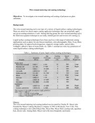
Characterization and
Dissolution of Ferroniobium
Aaron Den Boer
Supervisor: Dmitri Malakhov
McMaster University
November 20, 2012

Outline
‣ Introduction
‣ Problem Definition
‣ Completed Work – Characterization of FeNb
‣ Current Work – Modelling Solid Nb Dissolution in Liquid Fe
‣ Future Work – Validation of Binary Model
2

Introduction
• Microalloying produces steels (called High Strength Low Alloy
steels) with superior toughness, corrosion resistance, and increased
strength, as compared to some other steels
• Microalloying with elements such as Nb, Ti, and V improve these
properties through grain refinement, and solid solution and
precipitation hardening
3

Introduction
• Evolution of microalloyed HSLA steels has led to the development
of ferroalloy additions in steelmaking
• Microalloying is performed by adding ferroalloys to the liquid steel
during ladle metallurgy FeNb, FeTi, FeV
• One aim of ladle metallurgy is alloying to adjust for target chemical
analysis; the ladle temperature is around 1600°C
• Once these ferroalloys have assimilated into the melt, casting will
result in the formation of fine precipitates at late stages of
solidification
http://www.danieli.com
Porter, Repas, 1982
4

Introduction
• How do these fine precipitates form during solidification
i. “Homogenous” liquid melt
ii.
Phases with high melting
temperatures (i.e. Nb-C,
Ti-N, Ti-C-S) precipitate out
Fe – 0.05 Nb – 0.1 C
(Nb,Ti) (C,N)
Jun, Kang, Park, 2003
5

Ferroniobium Manufacturing
• A mixture containing alumina, sodium aluminate, iron and niobium
is heated up to 2200°C and held for several minutes
• The melt is completely liquid and cast into a mold or poured on a
flat surface where it solidifies.
• Since freezing of several tonnes of FeNb is characterized by a low
cooling rate, solidification is assumed to proceed according to the
Gulliver-Scheil formalism
• Thermo-Calc can be used to simulate the solidification behaviour
and predict the phase portrait of the Fe-Nb system
Sousa, 2002
6

Fe–Nb Phase Diagrams
TCFE2
TCFE6
Eutectic
Distectic
C14
µ
C14
µ
http://cst-www.nrl.navy.mil/lattice/index.html
Laves C14 → (Fe,Nb) 2 (Fe,Nb) 1
µ → (Fe,Nb) 7 (Nb) 2 (Fe,Nb) 4
7

Fe–Nb Phase Diagram TCFE2
2
T STEEL
1
BCC
2
µ
1
Voss, Palm, Stein, Raabe, 2011
8

Problem Definition
• Coarse Nb(C,N) and (Nb,Ti)(C,N) particles were observed on the
fracture surface of bend test specimens
• These coarse particles are detrimental to the mechanical properties
of HSLA steels
• Particle size: >10µm
Abraham, Klein, Bodnar, Dremailova, 2006
9

Problem Definition
• Abraham et al proposed that the coarse particles were inherited
from multiphase ferroalloys
i. Phases with high melting temperatures are released into melt
via disintegration of ferroalloy
ii. Finite time → non-homogeneous melt
µ Phase
BCC Phase
Abraham, Klein, Bodnar, Dremailova, 2006
10

Characterization of FeNb + 0.12 wt% C
ICP Analysis
&
Carbon/Sulphur Analysis
Element
wt%
Nb 68.14
Fe 29.38
C 0.12
(Ti, Cu, Al, Mn, P, Si) 2.37
Total 100.00
11

Nb–C Phase Diagram
FCC
HCP
M 2 C carbides, HCP structure
(Nb, Fe,…) 2 (C,N,Va) 1
MC carbides, FCC structure
(Nb, Fe,…) 1 (C, N, Va) 1
12

Characterization of FeNb + 0.12 wt% C
5
1
2
4
3
Location
Elements (at%)
Predicted
Fe Nb Ti Al Si Mn Phase
1 7.60 91.92 0.48 0.00 0.00 0.00 BCC
2 40.93 52.91 0.40 0.89 4.45 0.42 µ
3 35.34 62.16 0.89 0.48 0.83 0.31 η
4 1.92 96.94 1.14 0.00 0.00 0.00 HCP
5 11.09 13.94 0.94 72.94 0.92 0.18 Al203
FeNb + 0.12 wt% C
Phase Image Analysis TCFE2 EBSD
HCP (Red) 2.10 1.83 3.21
BCC (Yellow) 14.70 24.10 9.19
µ 80.80 73.85 87.6
Total 97.60 99.78 100
13

1600°C Isothermals for Fe–Nb–C
TCFE2
TCFE6
Nb C + L
2
Nb C + L
2
NbC + L
NbC + L
14

Characterization of FeNb + 0.7 wt% C
4
3
2
1
6
5
FeNb + 0.7 wt% C
Phase Image Analysis TCFE2
HCP 12.10 11.86
BCC 1.60 13.83
µ 78.50 73.13
LAVES 6.73 0.00
Total 98.93 98.82
Location
Elements (at%)
Predicted
Fe Nb Ti Al Si Mn Phase
1 0.89 98.47 0.64 0.00 0.00 0.00 HCP
2 43.00 51.71 0.41 0.88 3.59 0.41 µ
3 52.18 39.63 0.30 0.99 6.43 0.47 Laves
4 7.29 92.20 0.51 0.00 0.00 0.00 BCC
5 8.30 86.74 4.40 0.55 0.00 0.00 BCC
6 0.89 98.47 0.64 0.00 0.00 0.00 HCP
15

Modelling a Binary System
• Isothermal mass transfer phenomena governs kinetics of
dissolution – Mass Balance
• Determination of the time to complete dissolution (TCD) of pure
niobium spheres in pure liquid iron
16

Introduction to Model
• To solve total flux equation, one must know the precise
relationships between the total flux, N, and the fluid field quantities
(v, ρ)
N
A J
A vC
A
total flux
diffusive flux
bulk flux
• This mass transfer coefficient, k, is used to incorporate the bulk
flow and diffusive flow into one parameter
• Both stagnant and convective fluid conditions are bundled up into
dimensionless numbers, specifically the Sherwood number (Sh)
• In a stagnant fluid, v = 0 and Sh = 2 Sh = 2 + f(v,ρ)
Sh
kd
D
k
2R
D
k
DSh
2R
*
C C
*
NA
D kC C
R
17

Results: Stagnant Fluid
R R DC
C
2 L *
0
S
i
t
kA
i * *
s
C
C C C
exp
t
VL
18

It’s more complicated…
• If velocity is non-zero, how can one handle the total flux
formulation
N
A J
A vC
A
total flux
diffusive flux
bulk flux
• Fluid conditions are handled through the Sherwood number for
both natural and forced convection
19

Convective Fluid
• There are two types of convection that must be considered:
1. Natural Convection
o
the dissolving solid will develop concentration gradients near the
interface, forming a density gradient in the liquid
1/4
Sh20.59 Grm
Sc
R
final
dt
N 3/4
C
C R
Natural
R
0
RdR
1 2 0
t
final
2. Forced Convection
o A velocity field is applied and fixed externally on a system
Sh20.6Re
Sc
1/2 1/3
R
final
dt
F 1/2
C
C R
Forced
R
0
RdR
final
1 2 0
t
20

Results: Convective Fluid
21

Future Work
• Modelling ternary dissolution of Nb-C phases in pure liquid Fe
– Range of stoichiometry
– Solubility product and flux balance at interface
Experiments:
• Dissolution of Fe-Nb and Fe-Nb-C to validate the binary and ternary
models
22

Conclusions
• Thermodynamic databases should be used with caution in relation
to ferroalloys
• The poisonous effect of carbon in ferroniobium should not be
marginalized with respect to size and fraction of niobium carbides
• The solution of the dissolution equation for the Fe-Nb system with
different fluid conditions resulted in a noticeable effect on the TCD
and followed a consistent, logical pattern
• Consideration of the Fe-Nb-C system for modelling of dissolution
and experiments
23

The End…
• With gratitude to the following people and groups:
– Dr. Dmitri Malakhov
– Dr. Gord Irons
– Jim Garrett
– John Thomson
– Chris Butcher
– Doug Culley
– Ed McCaffery
– Xiaogang Li
– Fellow graduate students
– SRC
– CCEM
24

Meta-stable phase, η
2
1
Location
Elements (at%)
Predicted
Fe Nb Ti Al Si Mn Phase
1 34.48 62.46 0.77 0.56 1.73 0.00 ETA
2 35.19 61.02 0.67 0.59 2.52 0.00 ETA
2002 - THE IRON - NIOBIUM PHASE DIAGRAM AND THE VISCOSITY OF LIQUID - Korchemkina, Shunyaev 25

EBSD of FeNb + 0.7 wt% C
26

FeNb solidified at CBMM
27