Lp Norms and the Sinc Function - Faculty of Computer Science ...

L p Norms and the Sinc Function
D. Borwein, J. M. Borwein and I. E. Leonard
March 6, 2009
1 Introduction
The sinc function is a real valued function defined on the real line R by the following expression:
⎧
⎨sinx
if x ≠ 0
sinc(x) = x
⎩
1 otherwise
This function is important in many areas of computing science, approximation theory, and numerical analysis.
For example, it is used in interpolation and approximation of functions, approximate evaluation of transforms
(e.g. Hilbert, Fourier, Laplace, Hankel, and Mellon transforms as well as the fast Fourier transform). It is
used in finding approximate solutions of differential and integral equations, in image processing (it is the
Fourier transform of the box filter and central to the understanding of the Gibbs phenomenon [12]), in signal
processing and information theory. Much of this is nicely described in [7].
The first explicit appearance of the sinc function in approximation theory was probably in the use of the
Whittaker cardinal functions C(f, h) to approximate functions analytic on an interval or on a contour. Given
a function f which is defined on the real line R, the function C(f, h) is defined by
C(f, h) =
∞∑
k=−∞
f(kh)S(k, h)
whenever the series converges, where the stepsize h > 0 and where
S(k, h)(x) =
sin[( π (x − kh)]
h
π
h (x − kh) ,
that is, S(k, h)(x) = sinc ( π
h (x − kh)) . See, for example, [11].
The object of this note is to study the behavior and properties of the following function
I(p) = √ ∫ ∞
p
sin x
p
∣ x ∣ dx
∫ ∞
for 1 < p < ∞. Note that this function is only defined for p > 1, since
Indeed
∫ ∞
0
sin x
x dx = π 2
0
while
∫ ∞
0
0
sin x
∣ x ∣ dx = +∞,
sin x
dx is conditionally convergent.
x
see [12].
This integral arises, for example, in the L p approximation of real valued functions by Whittaker cardinal
functions, and is important in estimating the error made in the approximation. It also arises in many other
computational problems, and it is surprising that so little is known about it.
Various properties of the function I(p) are known. For example, the behavior of I(p) for large p is known:
∫
√ ∞
lim I(p) = lim p
p→∞ p→∞
0
1
∣
sinx
x
√ p
3π
∣ dx =
2

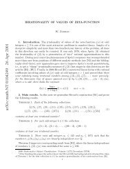
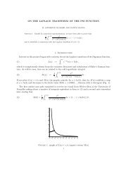
Figure 1: The function I on [2, 10]
This result, obtained independently by A. Meir and I. E. Leonard, is in principle not new (see equation 3).
We provide a self-contained proof below as part of our more general result in Theorem 1.
Also, for integer p, the integral
∫ ∞
0 x
can be calculated explicitly. In fact, for n ≥ 1 we have
∫ ∞
0
( ) n sinx
dx =
x
1
(n − 1)! ·
( ) p sin x
dx
⌊
π
n 2 ⌋
2 n ·
∑
( n
(−1) k k
k=0
) (n
− 2k
) n−1
This result is most definitely not new, it can be found in Bromwich [4, Exercise 22, p. 518], where it is
attributed to Wolstenholme, and in many other places—including two relatively recent articles on integrals
of more general products of sinc functions [2, 3].
Thus, if p is an even integer, then we have a closed form expression for I(p), and in this case the values of
I(p) can be calculated exactly:
I(p) = √ p
∫ ∞
0
( ) p sin x
dx = √ 1
p ·
x (p − 1)! · π
⌊ p 2 ⌋
2 p ·
∑
( p (p
(−1)
k) k ) p−1.
− 2k (1)
In particular I(2) = π/ √ 2, I(4) = 2π/3 and I(6) = 11 √ 6π/40. That said, this sum is very difficult to use
numerically for large p. Not only are the rational factors growing rapidly but it contains extremely large
terms of alternating sign and consequently dramatic cancelations. For example
I(36) = 731509401860533204925821188658871713
1063081066500632194410149314560000000 π,
and I(10) = Q 100 π where Q 100 is a rational number whose numerator and denominator both have roughly
150 digits. Similarly I(12) = Q 144 π where Q 144 is comprised of 240 digit integers. We also note that
numerical integration of I(p) even to single precision is not easy and so (1) provides a very good confirmation
of numerical integration results. We challenge the reader to numerically confirm the limit at infinity to 8
places.
The behavior of I(p) for intermediate values of p is not fully established. It had been conjectured that I(p)
had a global minimum at p = 4, however, (very) recent computations using both Maple and Mathematica
suggest that the global minimum, and unique critical point, is at approximately p = 3.36... as illustrated in
Figure 1.
√
Although it is known that lim I(p) = +∞, and that lim I(p) = 3π
p→1 + p→∞ 2
, it is not known precisely how the
√
3π
2
asymptote y = is approached, although both numerical and graphical evidence strongly suggest the
following conjecture:
k=0
2

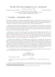
Figure 2: The function I and its limiting value on [2, 100]
Conjecture I is increasing for p above the conjectured global minimum near 3.36 and concave for p above
an inflection point near 4.469.
√
3π
This is shown in Figure 2 in which the dashed line has height
2
. Moreover, in Theorem 2 we shall prove
√ √ (
3π 2p 3π
I(p) >
2 2p + 1 > 1 − 1 )
, (2)
2 2p
for all p > 1.
We conclude this introduction by observing that one can derive the existence of an asymptotic expansion for
I(p) from a general result of Olver [10] on asymptotics of integrals using critical point theory and contour
integration. Specialized to our case, [10, Theorem 7.1, p. 127] (with q = 1 and p = log(sin(x)/x) on [−π, π])
establishes the existence of real constants c s such that
I(p) ∼ 1 ∫
√ π
p 2 ∣
∼
sin(x)
−π x
√
3π
2 − 3
√
3π
20 2
∣
p
dx
1
∞ p + ∑
s=2
c s
1
p s + · · · (3)
as p → ∞. From this one may deduce that I(p) is concave and increasing for sufficiently large values of
p—consistent with our stronger conjecture—as (3) may be differentiated termwise.
2 Our Main Results
In order to study the properties of the function I(p), we consider first the functions
∫ ∞
(
ϕ n (p) = log
sinx
n ∣
∣ x ∣)
·
sin x
p
∣ x ∣ dx
for p > 1 and n a nonnegative integer. We write
0
ϕ(p) = ϕ 0 (p) =
∫ ∞
0
sin x
∣ x ∣
In Lemma 1 below we confirm that ϕ(p) is analytic in a region containing (1, ∞) and that its n-th derivative
for p > 1 is given by ϕ (n) (p) = ϕ n (p).
Then in Theorem 1 we shall use induction to prove the following result for n a nonnegative integer:
√
3
lim
p→∞ pn+1 2 ϕ (n) (p) = (−1)
(n n
2 Γ + 1 )
.
2
p
dx.
3

The base case, n = 0, for our induction is established in Lemma 2 below. It uses Laplace’s method for
determining asymptotic behavior of an integral for large values of a parameter p, see, e.g., [6, p. 60].
Lemma 1 For p − 1 > z > 1 − p,
∞∑
ϕ(p − z) = (−1) n ϕ n (p) zn
n! .
n=0
In particular, ϕ(p) is analytic in a region containing (1, ∞) and its n-th derivative for p > 1 is given by
ϕ (n) (p) = ϕ n (p).
Proof. We have
ϕ(p − z) =
=
sin x
p−z ∫ ∞ ∞∑
(
∣
0 x ∣ dx = dx − log
sin x
n ∣
∣
0
x ∣)
·
sin x
p z n
∣ x ∣
(4)
n!
n=0
∞∑
∫ ∞
(
− log
sin x
n ∣
∣ x ∣)
·
sinx
p z n ∞
∣ x ∣ n! dx = ∑
(−1) n ϕ n (p) zn
n! , (5)
∫ ∞
n=0
0
n=0
the inversion of sum and integral in (4) being justified as follows:
Case i. p − 1 > z ≥ 0. All the terms involved are nonnegative.
Case ii. 0 > z > 1 − p. By Case i
ϕ(p − |z|) =
∫ ∞
0
∞∑
(
dx − log
sin x
n ∣
∣ x ∣)
·
sin x
p |z| n
∣ x ∣ n!
n=0
< ∞.
Thus (5) yields the Taylor series for ϕ(p − z) at z = 0, and the final conclusion follows.
Lemma 2
Proof. Let a > 0, then for p > 1 we have
I(p) = √ ∫ ∞
p
p
sin x
∣ x ∣ dx = √ p
We show first that
0
√
√ 3π
lim I(p) = lim pϕ(p) =
p→∞ p→∞ 2 . (6)
lim
p→∞
∫ a
0
∫
√ ∞
p ∣
a
p
sin x
∣ x ∣ dx + √ p
sinx
x
It suffices to consider the case 0 < a < 1; since for a ≥ 1, we have
∫
√ ∞
p ∫ p sin x
√ b
∣
a x ∣ dx ≤ lim p
b→∞ a
as p → ∞.
Now, for a < x < 1, we have
and it follows that
0 < √ p
∫ ∞
a
0 < sinx
x
< sina
a
∫ ∞
a
p
sin x
∣ x ∣ dx.
p
∣ dx = 0. (7)
√
1 p
x p dx = p − 1 ·
< 1,
sin x
p
∣ x ∣ dx ≤ √ ∫ 1
p
sin x
p
∣
a x ∣ dx + √ p
≤ (1 − a) √ p
sin a
p
∣ a ∣ +
1
−→ 0
ap−1 ∫ ∞
1
∣
sin x
x
√ p
p − 1 −→ 0
p
∣ dx
4

as p → ∞. This establishes (7).
We next use the following easily proved results [9, 8]:
1 − x2
6 ≤ sin x
x
≤ 1 − x2
6 + x4
120
for all real x, (8)
and ∫ 1
√ π
(1 − u 2 ) p Γ(p + 1)
du =
0
2 Γ ( ).
p + 3 (9)
2
where the equality is a special case of a beta-function evaluation (see also [12, Theorem 7.69]). It follows
from (8) and (9) that
∫ √ 6
0
p
sinx
∣ x ∣ dx ≥ √ 6
∫ 1
0
√
3π
(1 − u 2 ) p du =
2
Γ(p + 1)
Γ ( ),
p + 3 (10)
2
and hence that
liminf
p→∞
3π
I(p) ≥ lim
p→∞√
2
√ p Γ(p + 1)
Γ ( )
p + 3 . (11)
2
Now, in order to get an appropriate inequality for the limsup, we note that for any w > 1 such that
W = 2 √ √ (
5 1 −
w)
1 ≤ √ 6,
we have
whence
∫ W
0
sinx
∣ x ∣
p
sinx
x
≤ 1 − x2
6w
dx ≤ √ ∫ √6w W
6w (1 − u 2 ) p du ≤ √ 6w
0
for 0 < x < W, (12)
∫ 1
0
√
3πw
(1 − u 2 ) p Γ(p + 1)
du =
2 Γ ( ).
p + 3 (13)
2
It follows from (7) and (13) that
and therefore from (11) and (14), for w > 1 we have
lim
p→∞
√
3π
2
√ √ 3πw p Γ(p + 1)
limsup I(p) ≤ lim
p→∞ p→∞ 2 Γ ( )
p + 3 , (14)
2
√ p Γ(p + 1)
Γ ( )
p + 3 ≤ liminf I(p) ≤ limsup
p→∞
2
p→∞
Letting p → ∞ in (15), since for any a > 0, we have
lim
a→∞
from [8, Problem 2, p. 45] or (23), we obtain
√
3π
2 ≤ liminf
p→∞
√ (
a Γ a +
1
2
Γ(a + 1)
)
I(p) ≤ lim
p→∞
= 1,
I(p) ≤ limsup I(p) ≤
p→∞
for all w > 1. Finally, letting w → 1 + , we get the desired equation (6).
We are now ready for our more general result.
√ √ 3πw p Γ(p + 1)
2 Γ ( )
p + 3 . (15)
2
√
3πw
2 , (16)
5

Theorem 1 For all natural numbers n we have
lim
p→∞ pn+1 2 ϕ (n) (p) =
lim
p→∞ pn+1 2
∫ ∞
0
(
log
∣
= (−1) n √
3
2 Γ (
n + 1 2
sinx
n p
∣
x ∣)
·
sin x
∣ x ∣ dx
)
. (17)
Proof. The first equality was noted above. We proceed to establish equation (17) by induction. The proof
of the base case was given in Lemma 1.
For the inductive step of the proof, we assume that for a given nonnegative integer n, we have
√
3
lim
p→∞ pn+1 2 ϕ (n) (p) = (−1)
(n n
2 Γ + 1 )
.
2
It is easily verified that x < − log(1 − x) <
x
∣ ∣∣∣
1 − x for 0 < x < 1, and setting x = 1 − sint
p
t ∣ , that
1 −
sin t
p
∣ t ∣ < − log
sint
p 1 −
sin t
p
∣
t ∣
∣ t ∣ <
sin t
p
∣ t ∣
for all but countably many values of t.
For q > p + 1, multiplying these inequalities by the nonnegative term
(−1)
(log
n sint
n ∣
∣ t ∣)
·
sin t
q
∣ t ∣ ,
we have
) ( 0 ≤ (−1)
(log
n sin t
n ∣∣∣∣ sin t
∣ t ∣ t ∣
q
−
sin t
∣ t
) (
∣
∣p+q
< −(−1) n p log
∣
sin t
t
n+1 ∣
∣)
·
∣
) ( < (−1)
(log
n sin t
n ∣∣∣∣ sin t
∣ t ∣ t ∣
sin t
t
q−p
∣
q
−
sint
∣ t ∣
for the same values of t, and integrating over (0, ∞) yields
) (
)
(−1)
(ϕ n (n) (q) − ϕ (n) (p + q) ≤ −(−1) n p ϕ (n+1) (q) ≤ (−1) n ϕ (n) (q − p) − ϕ (n) (q) ,
q )
and hence
(−1) n ⎛
⎝ qn+1 2 ϕ (n) (q)
p q n+1 2
⎞
− (p + q)n+1 2 ϕ (n) (p + q)
⎠ ≤ −(−1) n qn+1+1 2 ϕ (n+1) (q)
p (p + q) n+1 2
q n+1+1 2
≤ (−1) n ⎛
⎝ (q − p)n+1 2 ϕ (n) (q − p)
p (q − p) n+1 2
⎞
− qn+1 2 ϕ (n) (q)
⎠. (18)
p q n+1 2
Now let q = kp, where k > 2 is fixed, then (18) becomes
⎛
⎞
(−1) n ⎝k q n+1 2 ϕ (n) (q) − k (p + q)n+1 2 ϕ (n) (p + q)
⎠ ≤
(1 + 1 k )n+1 2
≤
−(−1) n q n+1+1 2 ϕ (n+1) (q)
(−1) n ⎛
⎝k (q − p)n+1 2 ϕ (n) (q − p)
(1 − 1 k )n+1 2
⎞
− k q n+1 2 ϕ (n) (q) ⎠ .
6

Next let q → ∞, keeping k > 2 fixed, so that p → ∞ and q −p = (k −1)p → ∞. It follows from the inductive
hypothesis that
√
3
lim
q→∞ qn+1 2 ϕ (n) (q) = lim (p +
q→∞ q)n+1 2 ϕ (n) (p + q) = lim (q −
q→∞ p)n+1 2 ϕ (n) (q − p) = (−1)
(n n
2 Γ + 1 )
,
2
and therefore
⎛
k
⎝k −
(
1 +
1
k
Since
lim
k→∞
) n+
1
2
⎛
⎞
⎠
⎝k −
√ ( 3
2 Γ n + 1 )
2
k
(
1 +
1
k
) n+
1
2
⎞
≤
≤
⎠ = lim
liminf
q→∞
⎛
⎝
k→∞
(−1)n+1 q n+1+1 2 ϕ (n+1) (q) ≤ limsup (−1) n+1 q n+1+1 2 ϕ (n+1) (q)
q→∞
k
(
1 −
1
k
⎛
⎝
) n+
1
2
k
(
1 −
1
k
) n+
1
2
⎞
− k⎠
√ ( 3
2 Γ n + 1 )
. (19)
2
⎞
− k⎠ 1 − (1 + t) −n−1 2
= lim
= n + 1
t→0 t
2 ,
it follows from (19) that
√ ( 3
lim
q→∞ (−1)n+1 q n+1+1 2 ϕ (n+1) (q) = n + 1 ) (
Γ n + 1 ) √ ( 3
=
2 2 2 2 Γ n + 1 + 1 )
,
2
and this completes the proof of the inductive step.
3 Final Remarks
Our proof of Theorem 1 shows both that
lim
p→∞ pn+1 2 ϕ (n) (p) = a n (20)
exists and determines the value of a n . If we know in advance that the limit exists for every nonnegative
integer n, then we can use Lemmas 1 and 2 to write
√
lim p ϕ(p(1 + x)) = lim
p→∞
p→∞
∞∑
n=0
p n+1 2 ϕ (n) (p) xn
n! = √
3π/2
√ 1 + x
for 1 − 1 p > x > 1 p
− 1, and then justify the exchange of limit and sum, and expand the final term to obtain
∞∑
n=0
a n
x n
n! = ∞
∑
n=0
√
3
2 (−1)n Γ ( n + 1 2
) x n
n! .
Comparing coefficients of the above two exponential generating functions yields the desired valuation
a n =
√
3
2 (−1)n Γ ( n + 1 2)
. (21)
In fact, to justify the exchange by means of the series version of Lebesgue’s theorem on dominated convergence
one needs to establish something like ∣ ∣∣∣∣∣
p n+1 2 ϕ (n) (p)
n!
∣ ≤ M
with M a positive constant independent of n and p, and this requires an inequality such as the right-hand
side of (19) (with q replaced by p and n by n − 1) used in the given proof of Theorem 1.
7

Another way of determining the value of a n in (20) if we know it exists for every n, is to proceed via
L’Hospital’s rule as follows:
ϕ (n−1) (p)
a n−1 = lim = lim
p→∞
p −n+1 p→∞
2
ϕ (n) (p)
−(n − 1 2 )p−n−1 2
= − a n
n − 1 ,
2
whence, by Lemma 2,
which is (20) again.
a n = (−1) n a 0 n ∏
k=1
(
k − 1 ) √
3
=
2 2 (−1)n Γ ( )
n + 1 2
One advantage of our explicit proof of Lemma 2 over Olver’s asymptotic result in (3) is that it is easily
exploited to establish (2).
Theorem 2 For all p > 1 we have
√
3π
I(p) >
2
2p
2p + 1 > √
3π
2
(
1 − 1 )
. (22)
2p
Proof. For x > 0 and 0 < s < 1, Abromowitz and Stegun [1] records (as (5.6.4) in the new web version)
that
x 1−s Γ(x + 1)
<
Γ(x + s) < (x + 1)1−s . (23)
Hence, from (10) and (23) we obtain for p > 1 that
I(p)
> √ √ √
3π Γ(p + 1) 3π
p
2 Γ ( )
p + 3 =
2
2
√ √
3π 2p 3π
>
2 2p + 1 > 2
(
1 − 1
2p
√ p Γ(p + 1)
2p + 1 Γ ( )
p + 1 2
)
.
Here, for the penultimate inequality, we have used the left-hand inequality in (23) with x = p, s = 1/2.
Note that (22) implies that
‖sinc‖ p >
( √ ) 1/p 2 6p π
2p + 1
when sinc is viewed as a function in L p ([−∞, ∞]). We finish by observing that the lower bound is asymptotically
of the correct order, and leave as an open question whether similar explicit techniques to those in
Theorem 1 can be used to establish the second-order term in the asymptotic expansion (3) or the concavity
properties conjectured in the introduction.
References
[1] M. Abramowitz and I.A. Stegun, Handbook of Mathematical Functions, NBS (now NIST), 1965. See also
http://dlmf.nist.gov/.
[2] D. Borwein and J. M. Borwein, “Some remarkable properties of sinc and related integrals,” Ramanujan J., 5
(2001), 73–90.
[3] D. Borwein, J. M. Borwein, and B. Mares, “Multi-variable sinc integrals and volumes of polyhedra,”
Ramanujan J., 6 (2002), 189–208.
[4] T. J. Bromwich, Theory of Infinite Series, First Edition 1908, Second Edition 1926, Blackie & Sons, Glasgow.
[5] H. S. Carslaw, An Introduction to the Theory of Fourier’s Series and Integrals, Third Revised Edition, Dover
Publications Inc., New Jersey, 1950.
[6] N. G. de Bruijn, Asymptotic Methods in Analysis, Second Edition, North-Holland Publishing Co., Amsterdam,
1961.
8

[7] W. B. Gearhart and H. S. Schultz, “The function sin(x)
x
,” The College Mathematics Journal, 2 (1990), 90–99.
[8] P. Henrici, Applied and Computational Complex Analysis Volume 2, John Wiley & Sons, Inc., New York, 1977.
[9] I. E. Leonard and James Duemmel, “More–and Moore–Power Series without Taylor’s Theorem,” The
American Mathematical Monthly, 92 (1985), 588–589.
[10] F. W. J. Olver, Asymptotics and Special Functions (AKP Classics), Second Edition, AK Peters, Nattick, Mass,
1997.
[11] F. Stenger, Numerical Methods Based on Sinc and Analytic Functions, Springer Series in Computational
Mathematics 20, Springer–Verlag, New York, 1993.
[12] K. R. Stromberg, An Introduction to Classical Real Analysis, Wadsworth, Belmont, CA, 1981.
Acknowledgements We wish to thank Amram Meir and David Bailey for very useful discussions during
the preparation of this note.
9

David Borwein obtained two B.Sc. degrees from Witwatersrand University, one in engineering in 1945
and the other in mathematics in 1948. From University College London (UK) he received a Ph.D. in 1950
and a D.Sc. in 1960. He has been at the University of Western Ontario since 1963 with an emeritus title
since 1989. His main area of research has been classical analysis, particularly summability theory.
Department of Mathematics, The University of Western Ontario, London, ONT, N6A 5B7, Canada.
Email: dborwein@uwo.ca
Jonathan M. Borwein received his B.A. from the University of Western Ontario in 1971 and a D.Phil.
from Oxford in 1974, both in mathematics. He currently holds a Laureate Professorship at University of
Newcastle and a Canada Research Chair in the Faculty of Computer Science at Dalhousie University. His
primary current research interests are in nonlinear functional analysis, optimization, and experimental
(computationally-assisted) mathematics.
School of Mathematical and Physical Sciences, University of Newcastle, Callaghan, NSW 2308, Australia
and Faculty of Computer Science and Department of Mathematics, Dalhousie University, Halifax NS, B3H
2W5, Canada. Email: jonathan.borwein@newcastle.edu.au
Isaac E. Leonard received his B.A. and M.A. from the University of Pennsylvania in 1961 and 1963, both
in physics. He received his M.Sc. and Ph.D. from Carnegie-Mellon University in 1969 and 1973, both in
mathematics; and a B.Sc. in Computer Science from the University of Alberta in 1994. He currently holds
a position as a Sessional Lecturer with the Department of Mathematical and Statistical Sciences at the
University of Alberta, and has taught courses in the Computing Science and Electrical and Computer
Engineering Departments at the University of Alberta. His current research interests are in analysis of
algorithms and numerical analysis.
Department of Mathematical and Statistical Sciences, The University of Alberta, Edmonton, AB, T6G
2G1, Canada Email: isaac@math.ualberta.ca
10