Introduction to Matrix Algebra (pdf file)

Psychology 7291: Multivariate Statistics (Carey) 8/27/98 Matrix Algebra - 1 

Introduction to Matrix Algebra 

Definitions: 

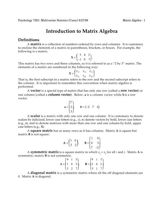
A matrix is a collection of numbers ordered by rows and columns. It is customary 

to enclose the elements of a matrix in parentheses, brackets, or braces. For example, the 

following is a matrix: 

5 8 2 

X = 

⎛ ⎜ ⎞ 

⎝ −1 0 7⎠ . 

This matrix has two rows and three columns, so it is referred to as a “2 by 3” matrix. The 

elements of a matrix are numbered in the following way: 

⎛ x 11 

x 12 

x 13 

X = ⎜ 

⎞ 

⎟ 

⎝ x 21 

x 22 

x 23 

⎠ 

That is, the first subscript in a matrix refers to the row and the second subscript refers to 

the column. It is important to remember this convention when matrix algebra is 

performed. 

A vector is a special type of matrix that has only one row (called a row vector) or 

one column (called a column vector). Below, a is a column vector while b is a row 

vector. 

⎛ 7⎞ 

a = 

2 

⎜ ⎟ , b = ( −2 7 4 ) 

⎝ 3⎠ 

A scalar is a matrix with only one row and one column. It is customary to denote 

scalars by italicized, lower case letters (e.g., x), to denote vectors by bold, lower case letters 

(e.g., x), and to denote matrices with more than one row and one column by bold, upper 

case letters (e.g., X). 

A square matrix has as many rows as it has columns. Matrix A is square but 

matrix B is not square: 

A = 1 6 ⎛ 1 9⎞ 

⎛ 

⎜ ⎞ 

⎟ , B = 0 3 

⎝ 3 2⎠ 

⎜ ⎟ 

⎝ 7 −2⎠ 

A symmetric matrix is a square matrix in which x ij 

= x ji 

for all i and j. Matrix A is 

symmetric; matrix B is not symmetric. 

⎛ 9 1 5⎞ 

⎛ 9 1 5⎞ 

A = 

⎜ 

1 6 2 

⎟ , B = ⎜ 

2 6 2 

⎟ 

⎝ 5 2 7⎠ 

⎝ 5 1 7⎠ 

A diagonal matrix is a symmetric matrix where all the off diagonal elements are 

0. Matrix A is diagonal.


⎛ 9 0 0⎞ 

A = 

0 6 0 

⎜ ⎟ 

⎝ 0 0 7⎠ 

An identity matrix is a diagonal matrix with 1s and only 1s on the diagonal. The 

identity matrix is almost always denoted as I. 

⎛ 1 0 0⎞ 

I = 

0 1 0 

⎜ ⎟ 

⎝ 0 0 1⎠ 

Matrix Addition and Subtraction: 

To add two matrices, they both must have the same number of rows and they both 

must have the same number of columns. The elements of the two matrices are simply 

added together, element by element, to produce the results. That is, for R = A+ B, then 

r ij 

= a ij 

+ b ij 

for all i and j. Thus, 

⎛ 

⎜ 

9 5 1⎞ 

⎛ 

⎟ = ⎜ 

1 9 −2⎞ 

⎛ 

⎟ + ⎜ 

8 −4 3⎞ 

⎟ 

⎝ −4 7 6⎠ 

⎝ 3 6 0⎠ 

⎝ −7 1 6⎠ 

Matrix subtraction works in the same way, except that elements are subtracted instead of 

added. 

Matrix Multiplication: 

There are several rules for matrix multiplication. The first concerns the 

multiplication between a matrix and a scalar. Here, each element in the product matrix is 

simply the scalar multiplied by the element in the matrix. That is, for R = aB, then 

r ij 

= ab ij 

for all i and j. Thus, 

⎛ 

8⎜ 

2 6 ⎞ ⎛ 

⎟ = ⎜ 

16 48⎞ 

⎟ 

⎝ 3 7⎠ 

⎝ 24 56⎠ 

Matrix multiplication involving a scalar is commutative. That is, aB = Ba. 

The next rule involves the multiplication of a row vector by a column vector. To 

perform this, the row vector must have as many columns as the column vector has rows. 

For example, 

⎛ 2⎞ 

( 1 7 5) 

4 

⎜ ⎟ 

⎝ 1⎠ 

is legal. However


⎛ 2⎞ 

⎜ 4⎟ 

( 1 7 5) 

⎜ 

⎜ 

1 

⎟ 

⎝ 6⎠ 

is not legal because the row vector has three columns while the column vector has four 

rows. The product of a row vector multiplied by a column vector will be a scalar. This 

scalar is simply the sum of the first row vector element multiplied by the first column 

vector element plus the second row vector element multiplied by the second column 

vector element plus the product of the third elements, etc. In algebra, if r = ab, then 

n 

r = ∑a i 

b i 

i =1 

Thus, 

⎛ 8⎞ 

( 2 6 3) 

1 

⎜ 

= 2∗8 + 6∗1 + 3∗4 = 34 

⎟ 

⎝ 4⎠ 

All other types of matrix multiplication involve the multiplication of a row vector 

and a column vector. Specifically, in the expression R = AB, 

r ij 

= a i • 

b •j 

where a i• 

is the ith row vector in matrix A and b •j 

is the jth column vector in matrix B. 

Thus, if 

A = 2 8 −1 ⎛ 1 7⎞ 

⎛ 

⎜ ⎞ 

⎟ ,and B = 9 −2 

⎝ 3 6 4⎠ 

⎜ ⎟ 

⎝ 6 3⎠ 

then 

⎛ 1⎞ 

r 11 

= a 1• 

b •1 

= ( 2 8 1) 

9 

⎜ 

= 2∗1 + 8∗9 + 1∗6 = 80 

⎟ 

⎝ 6⎠ 

and 

⎛ 7⎞ 

r 12 

= a 1• 

b •2 

= ( 2 8 1) 

−2 

⎜ 

= 2∗7 + 8∗(−2) + 1∗3 = 1 

⎟ 

⎝ 3⎠ 

and 

⎛ 1⎞ 

r 21 

= a 2• 

b •1 

= ( 3 6 4) 

9 

⎜ 

= 3∗1 + 6∗9 + 4∗6 = 81 

⎟ 

⎝ 6⎠ 

and


⎛ 7⎞ 

r 22 

= a 2• 

b •2 

= ( 3 6 4) 

−2 

⎜ 

= 3∗7 + 6∗(−2) + 4∗3 = 21 

⎟ 

⎝ 3⎠ 

Hence, 

⎛ 1 7⎞ 

⎛ 

⎜ 

2 8 −1⎞ 

⎟ 

9 −2 

⎝ 3 6 4⎠ 

⎜ ⎟ = ⎛ 

⎜ 

80 1 ⎞ 

⎟ 

⎝ 81 21⎠ 

⎝ 6 3⎠ 

For matrix multiplication to be legal, the first matrix must have as many columns as the 

second matrix has rows. This, of course, is the requirement for multiplying a row vector 

by a column vector. The resulting matrix will have as many rows as the first matrix and 

as many columns as the second matrix. Because A has 2 rows and 3 columns while B has 

3 rows and 2 columns, the matrix multiplication may legally proceed and the resulting 

matrix will have 2 rows and 2 columns. 

Because of these requirements, matrix multiplication is usually not commutative. 

That is, usually AB ≠ BA . And even if AB is a legal operation, there is no guarantee that 

BA will also be legal. For these reasons, the terms premultiply and postmultiply are often 

encountered in matrix algebra while they are seldom encountered in scalar algebra. 

One special case to be aware of is when a column vector is postmultiplied by a row 

vector. That is, what is 

⎛ −3⎞ 

4 

⎜ ⎟ 

( 8 2 ) 

⎝ 7⎠ 

In this case, one simply follows the rules given above for the multiplication of two 

matrices. Note that the first matrix has one column and the second matrix has one row, 

so the matrix multiplication is legal. The resulting matrix will have as many rows as the 

first matrix (3) and as many columns as the second matrix (2). Hence, the result is 

⎛ −3⎞ 

⎛ −24 −6⎞ 

⎜ 

4 

⎟ 

( 8 2 ) = 

32 8 

⎜ ⎟ 

⎝ 7⎠ 

⎝ 56 14⎠ 

Similarly, multiplication of a matrix times a vector (or a vector times a matrix) will also 

conform to the multiplication of two matrices. For example, 

⎛ 8 5⎞ 

⎛ 2⎞ 

⎜ 

6 1 

8 

⎟ ⎜ ⎟ 

⎝ 9 4⎠ 

⎝ 5⎠ 

is an illegal operation because the number of columns in the first matrix (2) does not 

match the number of rows in the second matrix (3). However,


⎛ 8 5⎞ 

⎛ 

6 1 

⎜ 

3 ⎞ 

⎛ 8∗3 + 5∗7⎞ 

⎛ 59⎞ 

⎟ 

⎜ = 

6∗3 +1∗7 

⎟ ⎝ 7⎠ 

⎜ ⎟ = 25 

⎜ ⎟ 

⎝ 9 4⎠ 

⎝ 9∗3 + 4∗7⎠ 

⎝ 55⎠ 

and 

⎛ 8 5⎞ 

( 2 7 3) 

6 1 

⎜ 

= 

⎟ 

( 2∗8 + 7∗6 + 3∗9 2∗5 + 7∗1 + 3∗4) = ( 85 29) 

⎝ 9 4⎠ 

The last special case of matrix multiplication involves the identity matrix, I. The 

identity matrix operates as the number 1 does in scalar algebra. That is, any vector or 

matrix multiplied by an identity matrix is simply the original vector or matrix. Hence, aI = 

a, IX = X, etc. Note, however, that a scalar multiplied by an identify matrix becomes a 

diagonal matrix with the scalars on the diagonal. That is, 

⎛ 

4⎜ 

1 0 ⎞ ⎛ 

⎟ = ⎜ 

4 0⎞ 

⎟ 

⎝ 0 1⎠ 

⎝ 0 4⎠ 

not 4. This should be verified by reviewing the rules for multiplying a scalar and a matrix 

given above. 

Matrix Transpose: 

The transpose of a matrix is denoted by a prime ( A ′ ) or a superscript t or T ( A t or 

A T ). The first row of a matrix becomes the first column of the transpose matrix, the 

second row of the matrix becomes the second column of the transpose, etc. Thus, 

A = 2 7 1 

⎛ 2 8⎞ 

⎛ 

⎜ ⎞ 

⎟ , and A 

t 

= 

7 6 

⎝ 8 6 4⎠ 

⎜ ⎟ 

⎝ 1 4⎠ 

The transpose of a row vector will be a column vector, and the transpose of a column 

vector will be a row vector. The transpose of a symmetric matrix is simply the original 

matrix. 

Matrix Inverse: 

In scalar algebra, the inverse of a number is that number which, when multiplied 

by the original number, gives a product of 1. Hence, the inverse of x is simple 1/x. or, in 

slightly different notation, x −1 . In matrix algebra, the inverse of a matrix is that matrix 

which, when multiplied by the original matrix, gives an identity matrix. The inverse of a 

matrix is denoted by the superscript “-1”. Hence, 

AA −1 = A −1 A = I 

A matrix must be square to have an inverse, but not all square matrices have an 

inverse. In some cases, the inverse does not exist. For covariance and correlation 

matrices, an inverse will always exist, provided that there are more subjects than there are 

variables and that every variable has a variance greater than 0.


It is important to know what an inverse is in multivariate statistics, but it is not 

necessary to know how to compute an inverse. 

Determinant of a Matrix: 

The determinant of a matrix is a scalar and is denoted as |A| or det(A). The determinant 

has very important mathematical properties, but it is very difficult to provide a 

substantive definition. For covariance and correlation matrices, the determinant is a 

number that is sometimes used to express the “generalized variance” of the matrix. That 

is, covariance matrices with small determinants denote variables that are redundant or 

highly correlated. Matrices with large determinants denote variables that are independent 

of one another. The determinant has several very important properties for some 

multivariate stats (e.g., change in R 2 in multiple regression can be expressed as a ratio of 

determinants.) Only idiots calculate the determinant of a large matrix by hand. We will 

try to avoid them. 

Trace of a Matrix: 

The trace of a matrix is sometimes, although not always, denoted as tr(A). The trace 

is used only for square matrices and equals the sum of the diagonal elements of the 

matrix. For example, 

⎛ 3 7 2⎞ 

tr 

-1 6 4 

⎜ ⎟ = 3 + 6 − 5 = 4 

⎝ 9 0 -5⎠ 

Orthogonal Matrices: 

Only square matrices may be orthogonal matrices, although not all square matrices 

are orthogonal matrices. An orthogonal matrix satisfied the equation 

AA t = I 

Thus, the inverse of an orthogonal matrix is simply the transpose of that matrix. 

Orthogonal matrices are very important in factor analysis. Matrices of eigenvectors 

(discussed below) are orthogonal matrices. 

Eigenvalues and Eigenvectors 

The eigenvalues and eigenvectors of a matrix play an important part in 

multivariate analysis. This discussion applies to correlation matrices and covariance 

matrices that (1) have more subjects than variables, (2) have variances > 0.0, and (3) are 

calculated from data having no missing values, and (4) no variable is a perfect linear 

combination of the other variables. Any such covariance matrix C can be mathematically 

decomposed into a product:


C = ADA -1 

where A is a square matrix of eigenvectors and D is a diagonal matrix with the 

eigenvalues on the diagonal. If there are n variables, both A and D will be n by n 

matrices. Eigenvalues are also called characteristic roots or latent roots. Eigenvectors 

are sometimes refereed to as characteristic vectors or latent vectors. Each eigenvalue 

has its associated eigenvector. That is, the first eigenvalue in D (d 11 

) is associated with the 

first column vector in A, the second diagonal element in D (i.e., the second eigenvalue or 

d 22 

) is associated with the second column in A, and so on. Actually, the order of the 

eigenvalues is arbitrary from a mathematical viewpoint. However, if the diagonals of D 

become switched around, then the corresponding columns in A must also be switched 

appropriately. It is customary to order the eigenvalues so that the largest one is in the 

upper left (d 11 

) and then they proceed in descending order until the smallest one is in d nn 

, 

or the extreme lower right. The eigenvectors in A are then ordered accordingly so that 

column 1 in A is associated with the largest eigenvalue and column n is associated with 

the lowest eigenvalue. 

Some important points about eigenvectors and eigenvalues are: 

1) The eigenvectors are scaled so that A is an orthogonal matrix. Thus, A T = A -1 , and 

AA T = I. Thus, each eigenvector is said to be orthogonal to all the other eigenvectors. 

2) The eigenvalues will all be greater than 0.0, providing that the four conditions 

outlined above for C are true. 

3) For a covariance matrix, the sum of the diagonal elements of the covariance 

matrix equals the sum of the eigenvalues, or in math terms, tr(C) = tr(D). For a correlation 

matrix, all the eigenvalues sum to n, the number of variables. Furthermore, in case you 

have a burning passion to know about it, the determinant of C equals the product of the 

eigenvalues of C. 

4) It is a royal pain to compute eigenvalues and eigenvectors, so don't let me catch 

you doing it. 

5) VERY IMPORTANT : The decomposition of a matrix into its eigenvalues and 

eigenvectors is a mathematical/geometric decomposition. The decomposition literally 

rearranges the dimensions in an n dimensional space (n being the number of variables) in 

such a way that the axis (e.g., North-South, East-West) are all perpendicular. This 

rearrangement may but is not guaranteed to uncover an important psychological construct 

or even to have a psychologically meaningful interpretation. 

6) ALSO VERY IMPORTANT : An eigenvalue tells us the proportion of total 

variability in a matrix associated with its corresponding eigenvector. Consequently, the 

eigenvector that corresponds to the highest eigenvalue tells us the dimension (axis) that 

generates the maximum amount of individual variability in the variables. The next 

eigenvector is a dimension perpendicular to the first that accounts for the second largest 

amount of variability, and so on.


Mathematical Digression: eigenvalues and eigenvectors 

An important mathematical formulation is the characteristic equation of a 

square matrix. If C is an n by n covariance matrix, the characteristic equation is 

|C - λI| = 0 (1.0) 

where λ is a scalar. Solving this equation for λ reveals that the equation is a nth degree 

polynomial of λ. That is, there are as many λs as there are variables in the covariance 

matrix. The n λs that are the roots of this polynomial are the eigenvalues of C. Because C 

is symmetric, all the λs will be real numbers (i.e., not complex or imaginary numbers), 

although some of the λs may be equal to or less than 0. The λs can be solved for in any 

order, but it is customary to order them from largest to smallest. 

To examine what is meant here, let C denote a two by two correlation matrix that 

has the form: 

⎛ 

⎜ 

1 ρ⎞ 

⎟ 

⎝ ρ 1⎠ 

Then the quantity C - λI may be written as 

⎛ 

C −λI= ⎜ 

1 ρ ⎞ ⎛ λ 0 

⎟ − ⎜ 

⎞ ⎛ 1 −λ 

⎟ = ⎜ 

⎝ ρ 1⎠ 

⎝ 0 λ⎠ 

⎝ ρ 

The determinant is 

ρ ⎞ 

⎟ 

1−λ⎠ 

C −λI = ( 1−λ) 2 −ρ 2 

So the equation that requires solution is 

(1−λ) 2 −ρ 2 = 0. 

This is a quadratic in λ. If we had three variables, it would be a cubic; and if there were 

four variables, it would be a quartic, etc. Solving for the quadratic gives 

λ = 1 ±ρ 

The largest root depends on the sign of ρ. For ρ > 0, then λ 1 

= 1 + ρ and λ 2 

= 1 - ρ. 

For each λ, one can define a nonzero vector a, such that 

( C −λI)a =0. 

The 0 to the right of the equal sign denotes a vector filled with 0s. Any number in a that 

satisfies this equation is called a latent vector or eigenvector of matrix C. Each eigenvector 

is associated with its own λ. Note that the solution to a is not unique because if a is 

multiplied by any scalar, the above equation still holds. Thus, there are an infinite set of 

values for a, although each solution will be a scalar multiple of any other solution. It is 

customary to normalize the values of a by imposing the constraint that a'a = 1. A latent 

vector subject to this constraint is called a normalized latent vector. 

Taking the two by two correlation matrix with ρ > 0, then


⎛ 

(C − λI)a = ⎜ 

1 −λ ρ ⎞ ⎛ 

⎟ ⎜ a 1⎞ 

⎛ (1−λ)a 

⎟ 1 

+ρa 

= ⎜ 

2 ⎞ 

⎟ = ⎜ 

⎛ 0 ⎞ ⎟ . 

⎝ ρ 1−λ⎠ 

⎝ a 2 

⎠ ⎝ (1− λ)a 2 

+ρa 1 ⎠ ⎝ 0⎠ 

or, by carrying out the multiplication, we find 

( 1−λ)a 1 

+ρa 2 

=0 

( 1−λ)a 2 

+ρa 1 

=0 

Now take the largest eigenvalue, l = 1 + r, and substitute. This gives 

ρ( a 2 

− a 1 

) = 0 

ρ( a 1 

− a 2 

) = 0 

Thus, all we know is that a 1 

= a 2 

. If we let a 1 

= 10, then a 2 

= 10; and if we let a 1 

= -.023, then 

a 2 

= -.023. This is what was meant above when it was said that there were an infinite 

number of solutions where any single solution is a scalar multiple of any other solution. 

By requiring that a'a = 1, we can settle on values of a 1 

and a 2 

. That is, if a 2 1 

+ a 2 2 

= 1 and a 1 

= 

a 2 

= a, say, then 2a 2 = 1 and a = .5 . So the first eigenvector will be a 2 by 1 column vector 

with both elements equaling .5 . 

For the second eigenvector, we substitute 1 - ρ for λ. This gives, 

ρ( a 1 

+ a 2 

) = 0 

Consequently, a 1 

= -a 2 

. One of the a's must equal .5 and the other must equal - .5 . It is 

immaterial which is positive and which is negative, but it is a frequent convention to 

make the first one (a 1 

) positive and the second negative. 

Note that the normalized eigenvectors of a two by two correlation matrix will 

always take on these values. The actual value of the correlation coefficient is irrelevant as 

long as it exceeds 0. 

Can you figure out the eigenvectors for a two by two matrix where ρ < 0

Introduction to Matrix Algebra (pdf file)

You also want an ePaper? Increase the reach of your titles

Delete template?

Save as template?