The Millikan Oil Drop Experiment

The Millikan Oil Drop Experiment
The Millikan Oil Drop experiment is one of the most famous experiments in the history of
physics. It is a very simple experiment but it is challenging to obtain good data. It will take
you many hours of observation to get the data for this experiment so you should prepare
carefully before you start trying to obtain numbers. If you just rush in, you will give up after a
few hours and start over, trying to figure out where everything went wrong. It will be helpful to
you if you read through this entire lab before starting to put the equipment together.
I. Theory
The electronic charge, or electrical charge carried by an electron, is one of the fundamental
constants in nature. Its initial determination is one of the most historically significant
experiments in physics. Around 1910, Robert Millikan, who later won a Nobel Prize,
developed an experiment using charged oil-drops to make the first accurate measurement of the
value of the electronic charge and to demonstrate its discreteness, or singleness of value. The
Millikan oil-drop procedure is still the most common method for this determination.
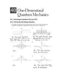
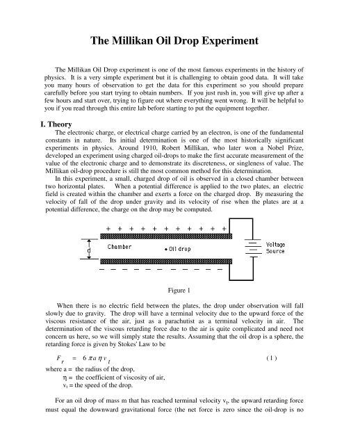
In this experiment, a small, charged drop of oil is observed in a closed chamber between
two horizontal plates. When a potential difference is applied to the two plates, an electric
field is created within the chamber and exerts a force on the charged drop. By measuring the
velocity of fall of the drop under gravity and its velocity of rise when the plates are at a
potential difference, the charge on the drop may be computed.
Figure 1
When there is no electric field between the plates, the drop under observation will fall
slowly due to gravity. The drop will have a terminal velocity due to the upward force of the
viscous resistance of the air, just as a parachutist as a terminal velocity in air. The
determination of the viscous retarding force due to the air is quite complicated and need not
concern us here, so we will simply state the results. Assuming that the oil drop is a sphere, the
retarding force is given by Stokes' Law to be
F = 6 π a η v
r
t
where a = the radius of the drop,
η = the coefficient of viscosity of air,
v t = the speed of the drop.
( 1 )
For an oil drop of mass m that has reached terminal velocity v t , the upward retarding force
must equal the downward gravitational force (the net force is zero since the oil-drop is no

longer accelerating) so that
F = 6π
aηv
= mg
r t
(2)
Suppose an electric field E is established between the plates is such a direction as to make
the drop move upward with a constant velocity of v E . The viscous force again opposes the
motion of the drop but now acts downward. If the oil drop has an electrical charge q when it
reaches constant velocity, the forces acting on the drop are again in equilibrium and
qE−
mg = 6πaηv
E
(3)
Solving the above equation for mg and setting it equal to the value for mg given in the
previous equation, we find that
mg = qE − 6π aηv
= 6πa
ηvt
E
or
(4)
6πa
η
q = +
E E
( v v ) (5)
t
The electric field between the plates is related to the distance d between the plates and the
applied voltage V by the equation
∆ V =Ed
(6)
Therefore,
6ππηd
q = +
∆V
E
( v v ) (7)
t
In the equation above, all quantities are known or measurable except a, the radius of the
drop. To obtain the value of a, Stokes' law can again be used. It states that when a small
sphere falls freely through a viscous medium it acquires a terminal velocity
v
t
2ga
2
=
( ρ − ρ )
oil
9η
air
where ρ oil = the density of the oil,
ρ air = the density of the air,
η = the viscosity of air.
The above equation can be solved for a:
(8)

a =
2g
9η
v
t
(9)
( ρ − ρ )
oil
air
Substituting this expression for a into the derived equation for q, we obtain the following
3
⎛18πd
⎞ η
q = ⎜ ⎟
+
⎝ ∆V
⎠ 2g
oil air
( ) ( ) ρ − ρ
v E
v t
v t
(10)
In his experiments Millikan found that the electronic charge resulting from measurements
seemed to depend somewhat on the size of the particular oil drop used and on the air pressure.
He suspected that the difficulty was inherent in Stoke's law which he found did not hold for
very small drops. It is necessary to make a correction, multiplying the velocities by the factor
( )
b
+
(11)
1 pa
where b = 6.17 x 10 -6 ,
p = the barometric pressure (in cm of Hg),
a = the radius of the drop.
(The value of this correction is so small that the rough value obtained from the previous
equation may be used).
The corrected charge on the drop is therefore given by
⎛18πd
⎞
q = ⎜ ⎟
⎝ ∆V
⎠
2g
η
3
⎛ +
⎝
b
pa
3
⎞ 2
⎛ ⎞
⎜v
+ v ⎟ ⎜1
⎟
(12)
( ρ − ρ ) ⎝ E g ⎠
v g
oil
air
⎠
where a in the last term is replace by Eqn. (9).
Even though this is a very complicated formula you can easily look at each component in it
and understand why it is there. Make sure that you understand the derivation of this formula
before you try to use it.
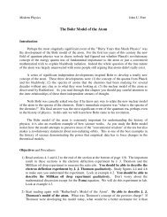
II. Apparatus
Figures 2 and 3 show the Millikan apparatus used in this experiment. The viewing
chamber consists of two parallel plates that are charged by the high voltage supply. The oil
drops are illuminated from behind by an incandescent light or a He-Ne laser and are observed
through the telescope. The voltmeter measures the potential between the two plates, and the
toggle switch on the condenser/input box changes the polarity of the plates. (In the upright
position, the switch can also disconnect the plates from the voltage supply.)
It is important to note the simplicity of this experimental setup. There is nothing happening
in this experiment other than an oil drop moving up and down between two charged plates. It
is remarkable that such a simple experiment can be used to measure an important physical
result.
If a He-Ne laser is used to illuminate the drops, an incandescent light should be placed to

the side of the telescope to illuminate the reference lines on the lens of the telescope. The laser
light, unlike the incandescent light, is highly directional and does not fall on the telescope lens.
The advantage of the laser is its ability to highly illuminate the oil drops and yet provide a
black background against which to view the drops.
Figure 2
(Note: the best set-up for this experiment will be obtained by trial and error (that's why we
call it an experiment!). You should try different arrangements to get the best optical
configuration. It will take you many hours of observation to obtain your results on the behavior
of the drops so you should spend some time understanding the optical arrangement).
Figure 3

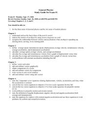
III. Procedures
To measure the velocities of the oil drops, it is necessary to calibrate the horizontal
markings on the telescope since you will use these to measure the displacement of the drops.
There are different ways to do this, one of which is the following: place an incandescent light
source behind the chamber (even if you will later be using a He-Ne laser) and adjust the
position of the telescope until you can see the inside of the chamber. Do not position the
telescope in line with the light source. Now take a piece of bare thin wire (approximately 20
gauge) and bend about 3 mm on one end at a right angle, as shown in Figure 4 on the next
page. Remove the oil hole cap and carefully insert the wire (bent end first) into the viewing
chamber through one of the small holes in the top plate. Move the telescope in and out using
the knob on the side until the wire comes into focus. Now measure the width of the wire
(W telescope ) using the reference lines on the telescope. (You may have to rotate the telescope so
that the lines are horizontal.) Remove the wire and measure its width (W micrometer ) using a
micrometer. (This is a common experimental tool that is frequently used to measure small
diameters) Find the distance x represented by each horizontal division.
Now carefully remove one of the glass plates on the viewing chamber and measure the
distance (d) between the top and bottom plates. Oil drops are introduced into the viewing
chamber by holding the nozzle of the atomizer against the small hole in the oil-hole cover and
gently squeezing the bulb. The oil drops acquire an electrical charge in the atomizing process.
(How does this happen) Once oil drops have entered the chamber, close the hole in the cap to
prevent air currents from disturbing the motion of the drops. At first a diffused light will be
seen which soon thins out and small individual bright spots (oil drops) appear. (The ones seen
first are usually too large to use and quickly fall out of the field of view.) Select one of the
slowest and follow its movements as the polarity of the plates is changed. Note that the
microscope appears to invert the motion so that a falling drop will appear to be rising and vice
versa. It is advisable to choose a drop which moves slowly when the electrical field is applied.
This indicates that the charge on the drop is small, probably being only a small multiple of that
of the electron.
Figure 4
If the drop is too small, it will not travel up and down in a straight line but will waver back
and forth, like a drunken sailor. This is due to Brownian motion, i.e. random collisions of air
molecules with the oil drop. If the drop tends to drift out of focus, move the telescope in and
out using the side knob. Practice following the drop up and down to develop the technique of

observing it and controlling its motion before starting to record data.
(Remember: it will take you hours of observation to obtain your final results so you should
not rush any of these procedures.)
When you are ready to begin collecting data, record the barometric pressure in centimeters
of mercury. Record the pressure again at the end of the experiment and use the average value.
Figure 5
We need to select oil drops with as few charges as possible for the best results. This will be
the oil drops that move the slowest when the voltage is applied. Select a satisfactory drop and
follow it up and down as long as possible while recording the time for the drop to move up
(down in the telescope) a given number of divisions. Occasionally record the voltage, which
should be constant, and the time for the drop to move down (up in the telescope) the same
number of divisions. Use the average of the latter for your calculations.
Measure the time of rise and fall of the drop for the same voltage several times, if possible.
Use the average. ( A sudden change in velocity indicates that the charge on the droplet or the
mass has suddenly changed, voiding the trial.) Do this for 4 or 5 different drops and for each
drop try 4 or 5 different voltages. (Hint: since your data is so rough for this experiment, you
need a lot of data to help reduce the experimental error).
IV. Analysis
1. Use a spreadsheet to make the following calculations. Calculate the terminal velocities of
rise, v E , and the terminal velocities of fall, v t for each oil drop and voltage.
2. Compute the approximate radius a for each oil drop from the appropriate equation in the
Theory section. The viscosity of the air may be taken to be 1.82 X 10 -5 Ns/m 2 although
you might want to look this up in a handbook. Use 9.80 m/s 2 for the acceleration of
gravity g, 890 kg/m 3 for the density of the oil, and 1.29 kg/m 3 for the density of air.
3. Compute the electrical charge q on the oil drop. Note that most quantities in the equation
remain constant during the experiment.
4. By a rough inspection of the data, determine the number n of electrons on the drop for each
charge calculated. This will be easy if the drop carried relatively few electrons, which was
the reason for selecting a drop that moved upward in the electric field at a slow rate.

5. Divide the charge by the number of electrons n which it carried to obtain a volume for the
charge on the electron. These values may vary but their average should be in close
agreement with the correct value of e (1.602 X 10 -19 C ) if the experiment has been
carefully performed.
6. Next we will all share our data to analyze the data a different way. If we have enough data
points (75 or so) and the number of charges is low we can plot a histogram and is a number
of peaks in the data that correspond to the number of charges.