Download Color Space Transformations - Nerim
Download Color Space Transformations - Nerim
Download Color Space Transformations - Nerim

Create successful ePaper yourself
Turn your PDF publications into a flip-book with our unique Google optimized e-Paper software.
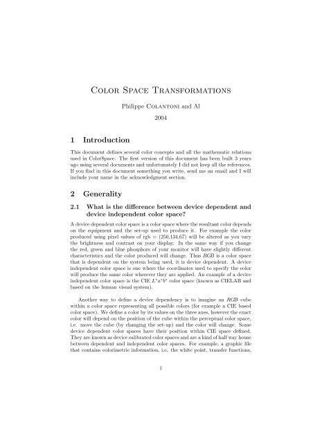
<strong>Color</strong> <strong>Space</strong> <strong>Transformations</strong><br />
Philippe Colantoni and Al<br />
2004<br />
1 Introduction<br />
This document defines several color concepts and all the mathematic relations<br />
used in <strong>Color</strong><strong>Space</strong>. The first version of this document has been built 3 years<br />
ago using several documents and unfortunately I did not keep all the references.<br />
If you find in this document something you write, send me an email and I will<br />
include your name in the acknowledgment section.<br />
2 Generality<br />
2.1 What is the difference between device dependent and<br />
device independent color space<br />
A device dependent color space is a color space where the resultant color depends<br />
on the equipment and the set-up used to produce it. For example the color<br />
produced using pixel values of rgb = (250,134,67) will be altered as you vary<br />
the brightness and contrast on your display. In the same way if you change<br />
the red, green and blue phosphors of your monitor will have slightly different<br />
characteristics and the color produced will change. Thus RGB is a color space<br />
that is dependent on the system being used, it is device dependent. A device<br />
independent color space is one where the coordinates used to specify the color<br />
will produce the same color wherever they are applied. An example of a device<br />
independent color space is the CIE L ∗ a ∗ b ∗ color space (known as CIELAB and<br />
based on the human visual system).<br />
Another way to define a device dependency is to imagine an RGB cube<br />
within a color space representing all possible colors (for example a CIE based<br />
color space). We define a color by its values on the three axes, however the exact<br />
color will depend on the position of the cube within the perceptual color space,<br />
i.e. move the cube (by changing the set-up) and the color will change. Some<br />
device dependent color spaces have their position within CIE space defined.<br />
They are known as device calibrated color spaces and are a kind of half way house<br />
between dependent and independent color spaces. For example, a graphic file<br />
that contains colorimetric information, i.e. the white point, transfer functions,<br />
1
and phosphor chromaticities, would enable device dependent RGB data to be<br />
modified for whatever device was being used - i.e. calibrated to specific devices.<br />
2.2 What is a color gamut <br />
A color gamut is the area enclosed by a color space in three dimensions. It<br />
is usual to represent the gamut of a color reproduction system graphically as<br />
the range of colors available in some device independent color space. Often the<br />
gamut will be represented in only two dimensions.<br />
2.3 What is the CIE System <br />
The CIE has defined a system that classifies color according to the HVS (the<br />
human visual system). Using this system we can specify any color in terms of<br />
its CIE coordinates.<br />
The CIE system works by weighting the spectral power distribution of an<br />
object in terms of three color matching functions. These functions are the sensitivities<br />
of a standard observer to light at different wavelengths. The weighting<br />
is performed over the visual spectrum, from around 360nm to 830nm in set<br />
intervals. However, the illuminant, the lighting and the viewing geometry are<br />
carefully defined, since these all affect the appearance of a particular color. This<br />
process produces three CIE tristimulus values, XYZ, which are the building<br />
blocks from which many color measurements are made.<br />
2.4 Gamma and linearity<br />
Many image processing operations, and also color space transforms that involve<br />
device independent color spaces, like the CIE system based ones, must<br />
be performed in a linear luminance domain. By this we really mean that the<br />
relationship between pixel values specified in software and the luminance of a<br />
specific area on the CRT display must be known. In most cases CRT have<br />
a non-linear response. The luminance of a CRT is generally modeled using a<br />
power function with an exponent, e.g. gamma, somewhere between 2.2 (NTSC<br />
and SMPTE specifications) and 2.8. This relationship is given as follows:<br />
luminance ∼ voltage γ<br />
Where luminance and voltage are normalized. In order to display image<br />
information as linear luminance we need to modify the voltages sent to the CRT.<br />
This process stems from television systems where the camera and receiver had<br />
different transfer functions (which, unless corrected, would cause problems with<br />
tone reproduction). The modification applied is known as gamma correction<br />
and is given below:<br />
NewV oltage = OldV oltage (1/γ)<br />
2
(both voltages are normalized and γ is the value of the exponent of the<br />
power function that most closely models the luminance-voltage relationship of<br />
the display being used.)<br />
For a color computer system we can replace the voltages by the pixel values<br />
selected, this of course assumes that your graphics card converts digital values<br />
to analogue voltages in a linear way. (For precision work you should check this).<br />
The color relationships are:<br />
R = a.(R ′ ) γ + b G = a.(G ′ ) γ + b B = a.(B ′ ) γ + b<br />
where R ′ , G ′ , and B ′ are the normalized input RGB pixel values and R, G,<br />
and B are the normalized gamma corrected signals sent to the graphics card.<br />
The values of the constants a and b compensate for the overall system gain and<br />
system offset respectively (essentially gain is contrast and offset is intensity).<br />
For basic applications the value of a, b and γ can be assumed to be consistent<br />
between color channels, however for precise applications they must be measured<br />
for each channel separately.<br />
3 Tristimulus values<br />
3.1 The concept of the tristimulus values<br />
The light that reaches the retina is absorbed by three different pigments that<br />
differ in their absorption spectra. Relative absorption spectra of the shortwavelength<br />
cone (blue) s(λ), middle-wavelength cone (green) m(λ) and longwavelength<br />
cone (red) l(λ) can be see figure 1.<br />
Figure 1: Human cones (and rods) absorption spectra<br />
If one pigment absorbs a photon which leads to its photoisomeration the information<br />
about the wavelength of the photon is lost (principle of univariance).<br />
Lights of different wavelengths are able to produce the same degree of isomerations<br />
(if their intensities are adjusted properly) and consequently produce equal<br />
sensations. The probability of isomeration of one pigment is not correlated with<br />
3
the probability of isomeration of another pigment. The probability of isomeration<br />
is just determined by the wavelengths of the incident photons. If we do<br />
not think about the influences of the spatial and temporal effects that influence<br />
perception, the sensation of color is determined by the number of isomerations<br />
in the three types of pigments. Therefore colors can be described by just three<br />
numbers, the tristimulus values, independent of their spectral compositions that<br />
lead to these three numbers.<br />
3.2 The Tristimulus Values<br />
The tristimulus values T for a complex light I(λ) (light that is not monochromatic)<br />
can be calculated for the specific primaries P with their corresponding<br />
color matching functions P i (λ):<br />
∫<br />
T 1 =<br />
λ<br />
∫<br />
P 1 (λ).I(λ).dλ T 2 =<br />
3.3 Consequences<br />
λ<br />
∫<br />
P 3 (λ).I(λ).dλ T 3 =<br />
λ<br />
P 2 (λ).I(λ).dλ<br />
1. The amount of excitation of the three pigment types for a complex light<br />
stimulus I(λ) can be calculated:<br />
∫<br />
S exc =<br />
λ<br />
∫<br />
s(λ).I(λ).dλ M exc =<br />
λ<br />
∫<br />
m(λ).I(λ).dλ L exc =<br />
λ<br />
l(λ).I(λ).dλ<br />
2. The amount of excitation of each pigment type to a stimulus P (λ) can be<br />
calculated:<br />
∫<br />
S exc =<br />
λ<br />
∫<br />
s(λ).P (λ).dλ M exc =<br />
λ<br />
∫<br />
m(λ).P (λ).dλ L exc =<br />
λ<br />
l(λ).P (λ).dλ<br />
Each primary has a defined overlap in the absorption spectra of the three<br />
pigments and consequently leads to a defined sensation. An increase in<br />
intensity of one primary reduces to the multiplication with a scalar for<br />
each pigment. Now, because of the principle of univariance, we can add<br />
the influences of the three primaries to the resulting excitations of the<br />
three pigment types.<br />
3. Because of 2, there exists a linear transformation between the tristimulus<br />
values of a set of primaries and the color space formed by the isomerations<br />
of the cone pigments.<br />
Tristimulus values describe the whole sensation of a color. There exist a lot<br />
of other possibilities to describe the sensation of color. For example it is possible<br />
to use something equivalent to cylinder coordinates where a color is expressed<br />
by hue, saturation and luminance. If the luminance or the absolute intensity of a<br />
color is not of interest then a color can be expressed in chromaticity coordinates.<br />
4
3.4 Chromaticity Coordinates<br />
In order to calculate the tristimulus values T of a light stimulus due to a set of<br />
primaries we need to know the spectral shape of the color matching functions<br />
and of the stimulus. The tristimulus values are calculated by the integration of<br />
the product of the color matching function and the stimulus over the wavelength.<br />
The tristimulus values describe the sensation of the stimulus due to the set of<br />
primaries including the absolute intensities of the three primaries needed to<br />
match the stimulus. Of course the luminance of that stimulus could be varied<br />
without changing the hue and saturation of the stimulus. This is reflected in the<br />
chromaticity coordinates c that form a two dimensional space thus luminance<br />
is ignored.<br />
T 1<br />
T 2<br />
T 3<br />
c 1 =<br />
c 2 =<br />
c 3 =<br />
T 1 + T 2 + T 3 T 1 + T 2 + T 3 T 1 + T 2 + T 3<br />
It is not necessary to mention the third coordinate because:<br />
3.5 Spectrum locus<br />
c 1 + c 2 + c 3 = 1<br />
We can read the tristimulus values for the spectral colors as the values of the<br />
color matching functions. For complex light stimuli we would have to integrate.<br />
After that we can calculate the chromaticity coordinates out of the tristimulus<br />
values. In CIE space the tristimulus values are called X, Y and Z, the chromaticity<br />
coordinates are called x and y. The curve of the chromaticity coordinates of<br />
the spectral colors is called the spectrum locus (fig. 2).<br />
The straight line connecting the blue part of the spectrum with the red part<br />
of the spectrum does not belong to the spectral colors, but it can be mixed out<br />
of the spectral colors just as all colors inside the spectrum locus.<br />
4 <strong>Color</strong> spaces definitions<br />
<strong>Color</strong> is the perceptual result of light in the visible region of the spectrum, having<br />
wavelengths in the region of 380 nm to 780 nm. The human retina has three<br />
types of color photoreceptor cells cone, which respond to incident radiation with<br />
somewhat different spectral response curves. Because there are exactly three<br />
types of color photoreceptor, three numerical components are necessary and<br />
theoretically sufficient to describe a color.<br />
Because we get color information from image files which contain only RGB<br />
values we have only to know for each color space the RGB to the color space<br />
transformation formulae.<br />
5
Figure 2: CIE 1931 xyY chromaticy diagram<br />
4.1 Computer Graphic <strong>Color</strong> <strong>Space</strong>s<br />
Traditionally color spaces used in computer graphics have been designed for<br />
specific devices: e.g. RGB for CRT displays and CMY for printers. They are<br />
typically device dependent.<br />
4.1.1 Computer RGB color space<br />
This is the color space produced on a CRT display when pixel values are applied<br />
to a graphic card or by a CCD sensor (or similar). RGB space may be displayed<br />
as a cube based on the three axis corresponding to red, green and blue (see<br />
fig. 3(a)).<br />
4.1.2 Printer CMY color space<br />
The CMY color model stands for Cyan, Magenta and Yellow which are the complements<br />
of Red, Green and Blue respectively. This system is used for printing.<br />
CMY colors are called ”subtractive primaries”, white is at (0.0, 0.0, 0.0) and<br />
black is at (1.0, 1.0, 1.0). If you start with white and subtract no colors, you get<br />
white. If you start with white and subtract all colors equally, you get black (see<br />
fig. 3(b)).<br />
4.2 CIE XYZ and xyY color spaces<br />
The CIE color standard is based on imaginary primary colors XYZ i.e. which<br />
don’t exist physically. They are purely theoretical and independent of devicedependent<br />
color gamut such as RGB or CMY . These virtual primary colors<br />
have, however, been selected so that all colors which can be perceived by the<br />
6
(a) RGB color space<br />
(b) CMY color space<br />
Figure 3: Visualization of RGB and CMY color spaces<br />
human eye lie within this color space.<br />
The XYZ system is based on the response curves of the three color receptors<br />
of the eye’s. Since these differ slightly from one person to another person, CIE<br />
has defined a ”standard observer” whose spectral response corresponds more or<br />
less to the average response of the population. This objectifies the colorimetric<br />
determination of colors.<br />
XYZ (fig. 4(a)) is a 3D linear color space, and it is quite awkward to work<br />
in it directly. It is common to project this space to the X + Y + Z = 1 plane.<br />
The result is a 2D space known as the CIE chromaticity diagram (see fig. 2).<br />
The coordinates in this space are usually called x and y and they are derived<br />
from XYZ using the following equations:<br />
x =<br />
X<br />
X + Y + Z<br />
y =<br />
Y<br />
X + Y + Z<br />
z =<br />
Z<br />
X + Y + Z<br />
As the z component bears no additional information, it is often omitted.<br />
Note that since xy space is just a projection of the 3D XYZ space, each point<br />
in xy corresponds to many points in the original space. The missing information<br />
is luminance Y. <strong>Color</strong> is usually described by xyY coordinates, where x and y<br />
determine the chromaticity and Y the lightness component of color (fig. 4(b)).<br />
4.2.1 RGB to CIE XYZ Conversion<br />
There are different mathematical models to transform RGB device dependent<br />
color to XYZ tristimulus values. Conversion from RGB to XYZ can take the<br />
form of a simple matrix transformation (equ. 2) or a more complex transformation<br />
depending of the hardware used (e.g. to acquire or to display color<br />
information).<br />
(1)<br />
7
In this section we will define how to compute a linear transformation model.<br />
This model may by a correct approximation for CCD sensor (RGB to XYZ<br />
transform) and CRT display (XYZ to RGB transform). But do not forget, this<br />
is only an approximate model.<br />
⎡ ⎤ ⎡ ⎤<br />
⎣ R G<br />
B<br />
⎦ = A.<br />
⎣ X Y<br />
Z<br />
We can use for example this transformation:<br />
⎡ ⎤ ⎡<br />
⎣ R G<br />
B<br />
⎦ = ⎣<br />
3.06322 −1.39333 −0.475802<br />
−0.969243 1.87597 0.0415551<br />
0.0678713 −0.228834 1.06925<br />
and the inverse transform simply uses the inverse matrix.<br />
⎡<br />
⎣<br />
X<br />
Y<br />
Z<br />
⎤<br />
⎡<br />
⎦ = ⎣<br />
3.06322 −1.39333 −0.475802<br />
−0.969243 1.87597 0.0415551<br />
0.0678713 −0.228834 1.06925<br />
⎦ (2)<br />
⎤<br />
⎦<br />
⎤<br />
⎦ .<br />
−1<br />
⎡<br />
⎣ X Y<br />
Z<br />
This is all very useful, but the interesting question is ”Where do these numbers<br />
come from”. Figuring out the numbers to put in the matrix is the hard<br />
part. The numbers depend on the color system of the output device we are<br />
using. The important parts of a color system are the x and y chromaticity<br />
coordinates and the luminance component of the primaries (xyY ). However, if<br />
we don’t know the Y values, which is often the case, then we have a problem.<br />
However, we can solve this problem if we know the chromaticity coordinates of<br />
the white point. In the previous example we have used a the color system which<br />
has the following specifications:<br />
⎡<br />
. ⎣<br />
Coordinate x Red y Red x Green y Green x Blue y Blue<br />
Value 0.64 0.33 0.29 0.60 0.15 0.06<br />
R<br />
G<br />
B<br />
⎤<br />
⎦<br />
⎤<br />
⎦<br />
Coordinate x W hite y W hite Y W hite<br />
Value 0.3127 0.3291 1<br />
These terms will be abbreviated to x r , y r , x g , y g , x b , y b , x w , y w and Y w . We<br />
know already that the relation 1 links the tristimulus values to the chromaticity<br />
coordinates.<br />
We can transform these relations:<br />
X = x y Y<br />
Z = z y Y<br />
The first step is to use these relationships to determine the luminance Y<br />
values. So we can calculate the tristimulus values as follows<br />
8
⎡<br />
⎢<br />
⎣<br />
X r = Y r<br />
y r<br />
x r X g = Y g<br />
y g<br />
x g X b = Y b<br />
y b<br />
x b<br />
Y r = Y r Y g = Y g Y b = Y b<br />
Z r = Yr<br />
y r<br />
z r<br />
Z g = Y g<br />
y g<br />
z g<br />
For the tristimulus values of the white point:<br />
Z b = Y b<br />
y b<br />
z b<br />
X w = x w<br />
yw<br />
Y w = Y w Z w = z w<br />
yw<br />
We now make the assumption that the sum of full intensity values of red<br />
green and blue will be white. Using this assumption we can write this relationship:<br />
⎧<br />
⎨<br />
⎩<br />
X w = X r + X g + X b<br />
Y w = Y r + Y g + Y b<br />
Z w = Z r + Z g + Z b<br />
We can then substitute the previous equations to the current one and then<br />
rewrite this latter as a matrix relationship:<br />
⎡ x w<br />
⎤ ⎡ x<br />
yw<br />
Y w<br />
r x g x b<br />
⎤ ⎡<br />
y r y g y b<br />
⎣ Y w ⎦ = ⎣ 1.0 1.0 1.0 ⎦ . ⎣ Y ⎤<br />
r<br />
Y g<br />
⎦<br />
z w<br />
y w<br />
Y w<br />
Y b<br />
z r<br />
y r<br />
z g<br />
y g<br />
This matrix can be re-written as follows:<br />
⎡<br />
⎣ Y ⎤ ⎡ x r x g x b<br />
⎤<br />
r<br />
y r y g y b<br />
Y g<br />
⎦ = ⎣ 1.0 1.0 1.0 ⎦<br />
Y b<br />
z r<br />
y r<br />
z g<br />
y g<br />
z b<br />
y b<br />
z b<br />
y b<br />
−1<br />
⎡<br />
. ⎣<br />
x w<br />
yw<br />
Y w<br />
Y w<br />
z w<br />
y w<br />
Y w<br />
We now have the luminance values Y r , Y g , Y b and we can substitute these<br />
values into the previous equations to find X r , X g , X b , Z r , Z g , and Z b . The final<br />
step is to define the relationship between tristimulus values and RGB values<br />
as follows. The RGB matrix R should be the result of a multiplication of the<br />
conversion matrix C by the tristimulus matrix T :<br />
⎡<br />
⎣ 1 1 0 0<br />
1 0 1 0<br />
1 0 0 1<br />
⎤<br />
⎦ =<br />
⎡<br />
⎣ <br />
<br />
<br />
⎤ ⎡<br />
⎦<br />
⎤<br />
⎦<br />
⎣ X ⎤<br />
w X r X g X b<br />
Y w Y r Y g Y b<br />
⎦<br />
Z w Z r Z g Z b<br />
Then the conversion matrix can be calculated as follows<br />
C = R ∗ T T ∗ (T ∗ T T ) −1<br />
If we follow this procedure using the values given in the previous example<br />
then we arrive at the following solution:<br />
⎡<br />
⎤<br />
3.06322 −1.39333 −0.475802<br />
C = ⎣ −0.969243 1.87597 0.0415551 ⎦<br />
0.0678713 −0.228834 1.06925<br />
9
(a) XYZ color space<br />
(b) xyY color space<br />
Figure 4: Visualization of XYZ and xyY color spaces<br />
4.2.2 Chromaticity coordinates of phosphors<br />
Name x r y r x g y g x b y b White point<br />
Short-Persistence 0.61 0.35 0.29 0.59 0.15 0.063 N/A<br />
Long-Persistence 0.62 0.33 0.21 0.685 0.15 0.063 N/A<br />
NTSC 0.67 0.33 0.21 0.71 0.14 0.08 Illuminant C<br />
EBU 0.64 0.33 0.30 0.60 0.15 0.06 Illuminant D65<br />
Dell 0.625 0.340 0.275 0.605 0.150 0.065 9300 K<br />
SMPTE 0.630 0.340 0.310 0.595 0.155 0.070 Illuminant D65<br />
HB LEDs 0.700 0.300 0.170 0.700 0.130 0.075 x w =.31 y w =.32<br />
4.2.3 Standard white points<br />
Name x w y w<br />
Illuminant A 0.44757 0.40745<br />
Illuminant B 0.34842 0.35161<br />
Illuminant C 0.31006 0.31616<br />
Illuminant D65 0.3127 0.3291<br />
Direct Sunlight 0.3362 0.3502<br />
Light from overcast sky 0.3134 0.3275<br />
Illuminant E 1/3 1/3<br />
4.3 A better model for RGB to CIE XYZ conversion<br />
<strong>Color</strong><strong>Space</strong> enables user to apply a more accurate model for RGB to CIE XYZ<br />
conversion. This model (equ. 3) includes an offset suitable to calibrate CCD or<br />
CMOS sensors.<br />
10
⎡<br />
⎣ X Y<br />
Z<br />
⎤<br />
⎦ = A.<br />
⎡<br />
⎣ R G<br />
B<br />
⎤<br />
⎦ +<br />
⎡<br />
⎣ X offset<br />
Y offset<br />
Z offset<br />
⎤<br />
⎦ (3)<br />
4.4 CIE L ∗ a ∗ b ∗ and CIE L ∗ u ∗ v ∗ color spaces<br />
There are based directly on CIE XYZ (1931) and are another attempt to<br />
linearize the perceptibility of unit vector color differences. there are non-linear,<br />
and the conversions are still reversible. <strong>Color</strong>ing information is referred to the<br />
color of the white point of the system. The non-linear relationships for CIE<br />
L ∗ a ∗ b ∗ (see equ. 4 and fig. 5(a)) are not the same as for CIE L ∗ u ∗ v ∗ (see equ. 7<br />
and fig. 5(b)), both are intended to mimic the logarithmic response of the eye.<br />
⎧<br />
⎪⎨<br />
⎪⎩<br />
L ∗ = 116<br />
(<br />
Y<br />
) 1<br />
3<br />
Y 0<br />
L ∗ =<br />
( )<br />
Y<br />
903.3<br />
[<br />
Y 0<br />
]<br />
a ∗ = 500 f( X X 0<br />
) − f( Y Y 0<br />
)<br />
[<br />
]<br />
b ∗ = 200 f( Y Y 0<br />
) − f( Z Z 0<br />
)<br />
− 16 if Y Y 0<br />
> 0.008856<br />
if Y Y 0<br />
≤ 0.008856<br />
(4)<br />
with {<br />
f(U) = U<br />
1<br />
3 if U > 0.008856<br />
f(U) = 7.787U + 16/116 if U ≤ 0.008856<br />
and<br />
U(X, Y, Z) =<br />
4X<br />
X + 15Y + 3Z et V (X, Y, Z) = 9Y<br />
X + 15Y + 3Z<br />
(5)<br />
(6)<br />
⎧<br />
⎪⎨<br />
⎪⎩<br />
L ∗ = 116<br />
(<br />
Y<br />
) 1<br />
3<br />
Y 0<br />
( )<br />
Y<br />
Y 0<br />
− 16 if Y Y 0<br />
> 0.008856<br />
L ∗ = 903.3<br />
]<br />
u ∗ = 13L<br />
[U(X, ∗ Y, Z) − U(X 0 , Y 0 , Z 0 )<br />
[<br />
]<br />
v ∗ = 13L ∗ V (X, Y, Z) − V (X 0 , Y 0 , Z 0<br />
if Y Y 0<br />
≤ 0.008856<br />
(7)<br />
4.5 <strong>Color</strong> spaces used in video standards<br />
Y UV and Y IQ are standard color spaces used for analogue television transmission.<br />
Y UV is used in European TVs (see fig. 6(a)) and Y IQ in North American<br />
TVs (NTSC) (see fig. 6(b)). Y is linked to the component of luminance, and<br />
U, V and I, Q are linked to the components of chrominance. Y comes from the<br />
standard CIE XYZ.<br />
11
(a) L ∗ a ∗ b ∗ color space<br />
(b) L ∗ u ∗ v ∗ color space<br />
Figure 5: Visualization of L ∗ a ∗ b ∗ and L ∗ u ∗ v ∗ color spaces<br />
(a) Y UV color space<br />
(b) Y IQ color space<br />
Figure 6: Visualization of Y UV and Y IQ color spaces<br />
12
⎧<br />
⎨<br />
⎩<br />
⎧<br />
⎨<br />
⎩<br />
RGB to Y UV transformation<br />
Y = 0.299 × R + 0.587 × G + 0.114 × B<br />
U = −0.147 × R − 0.289 × G + 0.436 × B<br />
V = 0.615 × R − 0.515 × G − 0.100 × B<br />
RGB to Y IQ transformation<br />
Y = 0.299 × R + 0.587 × G + 0.114 × B<br />
I = 0.596 × R − 0.274 × G − 0.322 × B<br />
Q = 0.212 × R − 0.523 × G + 0.311 × B<br />
With these formulae the Y range is [0; 1], but U, V, I, and Q can be as well<br />
negative as positive.<br />
Y CbCr (see fig. 4.5) is a color space similar to Y UV and Y IQ. The transformation<br />
formulae for this color space depend on the recommendation used.<br />
We use the recommendation Rec 601-1 which gives the value 0.2989 for red, the<br />
value 0.5866 for green and the value 0.1145 for blue.<br />
Figure 7: Y CbCr color space<br />
⎧<br />
⎨<br />
⎩<br />
RGB to Y CbCr transformation<br />
Y = 0.2989 × R + 0.5866 × G + 0.1145 × B<br />
Cb = −0.1688 × R − 0.3312 × G + 0.5000 × B<br />
Cr = 0.5000 × R − 0.4184 × G − 0.0816 × B<br />
4.6 Linear transformations of RGB<br />
4.6.1 I 1 I 2 I 3 color space<br />
Ohta [3] introduced, after a colorimetric analysis of 8 images, this color space.<br />
This color space is a linear tranformation of RGB (see fig. 4.6.1).<br />
13
Figure 8: I 1 I 2 I 3 color space<br />
RGB to I 1 I 2 I 3 transformation<br />
⎧<br />
⎨ I 1 = 1 3<br />
(R + G + B)<br />
I 2 = 1<br />
⎩<br />
2<br />
(R − B)<br />
I 3 = 1 4<br />
(2G − R − B)<br />
4.6.2 LSLM color space<br />
This color space is a linear transformation of RGB based on the opponent signals<br />
of the cones: black–white, red–green, and yellow–blue (see fig. 4.6.2).<br />
⎧<br />
⎨<br />
⎩<br />
RGB to LSLM transformation<br />
L = 0.209(R − 0.5) + 0.715(G − 0.5) + 0.076(B − 0.5)<br />
S = 0.209(R − 0.5) + 0.715(G − 0.5) − 0.924(B − 0.5)<br />
LM = 3.148(R − 0.5) − 2.799(G − 0.5) − 0.349(B − 0.5)<br />
4.7 HSV and HSI color spaces<br />
The representation of the colors in the RGB and CMY color spaces are designed<br />
for specific devices. But for a human observer, they have not accurate definitions.<br />
For user interfaces a more intuitive color space is preferred. Such color<br />
spaces can be:<br />
• HSI ; Hue, Saturation and Intensity, which can be thought of as a RGB<br />
cube tipped up onto one corner (see fig. 10(b) and equ. 8).<br />
14
Figure 9: LSLM color space<br />
(a) HSV color space<br />
(b) HSI color space<br />
Figure 10: Visualization of HSV and HSI<br />
15
RGB to HSI transformation<br />
⎧<br />
⎨ H = arctan( β α )<br />
S = √ α<br />
⎩<br />
2 + β 2<br />
I = (R + G + B)/3<br />
(8)<br />
with<br />
{ α = R −<br />
1<br />
2<br />
(G + B)<br />
β = √ 3<br />
2<br />
(G − B)<br />
• There is different way to compute the HSV (Hue, Saturation and Value)<br />
color space [4]. We use the following algorithm 4.7.<br />
RGB to HSV transformation<br />
1 if (R > G) then Max = R; Min = G; position = 0;<br />
2 else Max = G; Min = R; position = 1;<br />
3 fi<br />
4 if (Max < B) then Max = B; position = 2 fi<br />
5 if (Min > B) then Min = B; fi<br />
6 V = Max;<br />
7 if (Max ≠ 0) then S = Max−Min<br />
Max<br />
;<br />
8 else S = 0;<br />
9 fi<br />
10 if (S ≠ 0) then<br />
11 if (position = 0)<br />
12 then H = 1 + G−B<br />
Max−Min ;<br />
13 else if (position = 1);<br />
14 then H = 3 + B−R<br />
Max−Min ;<br />
15 else H = 5 + R−G<br />
Max−Min ;<br />
16 fi<br />
17 fi<br />
The polar representation of HSV (see fig. 11(a)) and HSI (see fig. 11(b))<br />
color spaces leads a new visualization model of these color spaces (suitable for<br />
color selection).<br />
4.8 LHC and LHS color spaces<br />
The L ∗ a ∗ b ∗ (and L ∗ u ∗ v ∗ ) has the same problem as RGB, they are not very<br />
interesting for user interface. That’s why you will prefer the LHC equa. 9 (and<br />
LHS equa. 10), a color space based on L ∗ a ∗ b ∗ (and LHS). LHC stand for<br />
Luminosity , Chroma and Hue.<br />
16
(a) HSV color space (polar representation)<br />
(b) HSI color space (polar representation)<br />
Figure 11: Visualization of HSV and HSI color spaces (polar representation)<br />
⎧<br />
⎪⎨<br />
⎪⎩<br />
⎧<br />
⎪⎨<br />
⎪⎩<br />
L ∗ a ∗ b ∗ to LHC transformation<br />
L = L ∗<br />
C = √ a ∗2 + b ∗2<br />
H = 0 whether a ∗ = 0<br />
H = (arctan(b ∗ /a ∗ ) + k.π/2)/(2π)<br />
whether a ≠ 0 (add π/2 to H if H < 0)<br />
and k = 0 if a ∗ >= 0 and b ∗ >= 0<br />
or k = 1 if a ∗ > 0 and b ∗ < 0<br />
or k = 2 if a ∗ < 0 and b ∗ < 0<br />
or k = 3 if a ∗ < 0 and b ∗ > 0<br />
L ∗ u ∗ v ∗ to LHS transformation<br />
L = L ∗<br />
S = 13 √ (u ∗ − u ∗ w) 2 + (u ∗ − u ∗ w) 2<br />
H = 0 whether u ∗ = 0<br />
H = (arctan(v ∗ /u ∗ ) + k.π/2)/(2π)<br />
whether u ≠ 0 (add π/2 to H if H < 0)<br />
and k = 0 if u ∗ >= 0 and v ∗ >= 0<br />
or k = 1 if u ∗ > 0 and v ∗ < 0<br />
or k = 2 if u ∗ < 0 and v ∗ < 0<br />
or k = 3 if u ∗ < 0 and v ∗ > 0<br />
(9)<br />
(10)<br />
In order to have a correct visualization (with a good dynamic) of LHS and<br />
LHC color spaces we used the following color transformations:<br />
17
L ∗ a ∗ b ∗ to LHC transformation used in <strong>Color</strong><strong>Space</strong><br />
⎧<br />
L = L<br />
⎪⎨<br />
∗<br />
C = √ a ∗2 + b ∗2<br />
H = 0 whether a ∗ = 0<br />
⎪⎩<br />
H = 180<br />
π<br />
(π + arctan(<br />
b∗<br />
a ∗ )<br />
L ∗ u ∗ v ∗ to LHS transformation used in <strong>Color</strong><strong>Space</strong><br />
⎧<br />
L = L<br />
⎪⎨<br />
∗<br />
S = 1.3 √ (u ∗ − u ∗ w) 2 + (v ∗ − vw) ∗ 2<br />
H = 0 whether u ∗ = 0<br />
⎪⎩<br />
H = 180<br />
π<br />
(π + arctan(<br />
v∗<br />
u ∗ )<br />
(11)<br />
(12)<br />
(a) LHC color space<br />
(b) LHS color space<br />
Figure 12: Visualization of LHC and LHS color spaces<br />
4.9 Spectral (λSY ) color space<br />
λSY is a color space representation based on brightness, dominant wavelength<br />
and saturation attributes. λSY color coordinates are defined from xyY color<br />
coordinates.<br />
Let us consider the xy chromaticy diagram given by Figure 13(b). Then, any<br />
real color X that lies within the region enclosed by the spectrum locus line and<br />
upper the lines BW and W R can be considered to be a mixture of illuminant<br />
W and spectrum light of its dominant wavelength λ d which is determined by<br />
extending the line W X until it intersects the spectrum locus [9].<br />
Any color Y that lies on the opposite side of the illuminant point and below<br />
the lines BW and W R can be described both by a dominant wavelength λ d and<br />
18
λd<br />
Green<br />
λ d<br />
Green<br />
x<br />
x smax<br />
Spectrum locus<br />
x c<br />
Spectrum locus<br />
x<br />
λa−d<br />
White<br />
White<br />
Blue<br />
Red<br />
Blue<br />
y<br />
y s max<br />
Red<br />
(a)<br />
(b)<br />
(c)<br />
(d)<br />
Figure 13: λSY color space transformation.<br />
19
y its complementary wavelength λ c d<br />
which is determined by extending the line<br />
Y W until it intersects the line BR (i.e. the purple line).<br />
The saturation S is determined in the xy chromaticity diagram, either by<br />
the relative distance of the sample point and the corresponding spectrum point<br />
from the illuminant point, either by the relative distance of the sample point<br />
and the corresponding purple point from the illuminant point.<br />
5 Decorrelated hybrid color spaces<br />
The basic idea of hybrid color spaces is to combine either adaptively, either<br />
interactively, different color components from different color spaces to: (a) increase<br />
the effectiveness of color components to discriminate color data, and (b)<br />
reduce rate of correlation between color components [2].<br />
It is established that we can all the more reduce, from K to 3, the number<br />
of color dimensions that: (a) most of color spaces are linked the ones to the<br />
others, either by linear transformations or by non-linear transformations, and<br />
(b) all color spaces are defined by a 3 dimensional system.<br />
(a) (b) (c) (d) (e)<br />
(f) (g) (h) (i) (j)<br />
Figure 14: (a) RGB <strong>Color</strong> image, made of 6 regions (Brown, Orange, Yellow,<br />
Pink, Green and Dark Green), projected on different color components. (b),<br />
(c), (d) R, G, B projections. Among the three R, G, B color components, at<br />
most 3 regions can be identified with the component G. (e), (f), (g) Y, C b , C r<br />
projections. Among the three Y, C b , C r color components, at most 3 regions can<br />
be identified with the component Y . (h), (i), (j) H, S, V projections. Among<br />
the three H, S, V color components, at most 3 regions can be identified with<br />
the component H. In combining G, Y, H color components, all regions can be<br />
identified.<br />
Considering that there is a high redundancy between colors components it<br />
is, in a general way, quite difficult to define criteria of analysis to compute au-<br />
20
tomatically the most relevant color components corresponding to a selected set<br />
of color components. That is the reason why, in order to build a hybrid color<br />
space, based on K ′ color components, from K selected color components, such<br />
as K ′
(a) Parrot image<br />
(b)<br />
(c)<br />
(d)<br />
Figure 16: Decorrelated hybrid color spaces examples on parrot image<br />
22
6 Decorrelated hybrid color spaces applied to<br />
image database<br />
6.1 Decorrelated hybrid color spaces: an extension<br />
We have introduced the hybrid construction scheme in the precedent paragraph,<br />
based on one initial image. This strategy can be easily applied to a list of images,<br />
considering the set of images as one unique image.<br />
We will use the following notations, and we will suppose (for simplicity of formulæ<br />
only) all color spaces are normalized.<br />
• S the set of n images and S l the l-th image.<br />
• K the set of selected color spaces components and K i the i-th component.<br />
• K l i (x, y) the corresponding value of pixel (x, y) of component K i of image<br />
S l .<br />
• Size (S l ) the size in pixel of the image S l .<br />
Let introduce the Sum and Cross matrix, defined by:<br />
Sum l i = ∑<br />
xy∈S l<br />
K l i(x, y)<br />
Cross l ij = ∑<br />
xy∈S l<br />
K l i(x, y) ∗ K l j(x, y)<br />
We note, that for one image S l , the covariance is then defined by:<br />
Cov l ij = Crossl ij<br />
Size (S l ) −<br />
Suml i<br />
Size (S l ) ×<br />
Then, to expand the formula to n images:<br />
∑<br />
1≤l≤n<br />
Cov ij =<br />
Crossl ij<br />
∑<br />
1≤l≤n Size (S l) −<br />
∑<br />
1≤l≤n Suml i<br />
∑<br />
1≤l≤n Size (S l) ×<br />
Suml j<br />
Size (S l )<br />
∑<br />
1≤l≤n Suml j<br />
∑<br />
1≤l≤n Size (S l)<br />
At this point, the computation of the hybrid color space follows the previously<br />
cited steps:<br />
4. principal component analysis;<br />
5. selection of the 3 most significant axis.<br />
We have developed via ICobra and <strong>Color</strong><strong>Space</strong> applications a web interface<br />
system 3 [14] to manage these hybrid color spaces. The process is divided in two<br />
steps:<br />
3 Available at: http://www.icobra.info/hybrid.php<br />
23
• Off-line computation. This part intends to compute the main portion of<br />
calculus required by the hybrid color space computation.<br />
• Online interface. This part intends, via the interface, to select color spaces<br />
components and images, to complete the calculus, and, then, to show the<br />
selected image in the computed hybrid space.<br />
Before describes rapidly these two parts, we can note: all color spaces are normalized<br />
during the computation (there is a scale rapport from 1 to 200 between<br />
some spaces); the transfer values (primaries and white settings) used are, at this<br />
moment, still approximation.<br />
6.2 Off-line computation<br />
Figure 17: Off-line scheme<br />
The figure 17 illustrates the off-line computation. For each image, we will<br />
compute and store:<br />
• for each couple of color spaces components, the Cross value corresponding.<br />
It results a m × m matrix, where t is the number of possible color spaces<br />
components, presently 72 (3 × 24) components.<br />
• for each color spaces components, the Sum value corresponding. It results<br />
a vector of size m.<br />
• the size of image.<br />
6.3 Online interface<br />
As shown in 17 the application may be split into several sections:<br />
• World Wide Web Interface, as figure 19 illustrates. It permits:<br />
– to browse the different image databases;<br />
– to select by clicks a list of images. An empty list means that the<br />
decorrelated hybrid color space is computed on self-image, as usual;<br />
24
Figure 18: Overall online scheme<br />
Figure 19: WWW interface<br />
25
– to select a list of color spaces components;<br />
– to choose the mode of visualization: 2D image, 3D, or 3D histogram;<br />
– to launch <strong>Color</strong><strong>Space</strong> with the selected parameters;<br />
• A computational part: the final covariance matrix is computed, using<br />
pre-calculated data;<br />
• A CSI file generation: a csi file (<strong>Color</strong> <strong>Space</strong> Interface) is generated, including<br />
all settings and information in order to compute the PCA and<br />
displaying the selected visualization;<br />
• <strong>Color</strong><strong>Space</strong> launching: <strong>Color</strong><strong>Space</strong> is launched by the browser (application/csi<br />
mime-type bind) with the csi file as parameter. The software<br />
computes the PCA, and renders the selected visualization.<br />
Figure 20 illustrates this tool within some screenshots using different images<br />
and color spaces components.<br />
7 References and lectures<br />
[1] P. Colantoni and A. Trémeau, “3d visualization of color data to analyze<br />
color images,” in The PICS Conference, (Rochester, USA), May 2003.<br />
[2] N. Vandenbrouke, L. Macaire, and J. G. Postaire, “<strong>Color</strong> pixels classification<br />
in a hybrid color space,” in Proceedings of IEEE, pp. 176–180,<br />
1998.<br />
[3] Y. I. Ohta, T. Kanade, and T. Sakai, “<strong>Color</strong> information for region segmentation,”<br />
Computer Graphics and Image Processing, vol. 13, pp. 222–<br />
241, 1980.<br />
[4] D. F. Rogers, Procedural Elements for Computer Graphics. Mc Graw Hill,<br />
1985.<br />
[5] G. A. Agoston, <strong>Color</strong> Theory and its Application in Art and Design. Optical<br />
Sciences, Springer-Verlag, 1987.<br />
[6] CIE, “Parametric effects in colour-difference evaluation,” Tech. Rep. 101,<br />
Bureau Central de la CIE, 1993.<br />
[7] CIE, “Technical collection 1993,” tech. rep., Bureau Central de la CIE,<br />
1993.<br />
[8] CIE, “Industrial colour-difference evaluation,” Tech. Rep. 116, Bureau<br />
Central de la CIE, 1995.<br />
[9] D. L. MacAdam, <strong>Color</strong> Measurement, theme and variation. Optical Sciences,<br />
Springer-Verlag, second revised ed., 1985.<br />
[10] G. Wyszecki and W. S. Stiles, <strong>Color</strong> Science: Concepts and Methods,<br />
Quantitative Data and Formulae. John Wiley & sons, second ed., 1982.<br />
26
(a) Original image (b) Selected components<br />
(c) Decorrelated hybrid color<br />
and images space representation<br />
list<br />
(d) (e) (f)<br />
(g) (h) (i)<br />
Figure 20: Decorrelated hybrid color spaces: some examples<br />
27
[11] H. R. Kang, <strong>Color</strong> Technology for Electronic Imaging Devices. SPIE<br />
Optical Engineering Press, 1997.<br />
[12] K. N. Plataniotis and A. N. Venetsanopoulos, <strong>Color</strong> Image Processing<br />
and Application. Springer, 2000.<br />
[13] R. Hall, Illumination and <strong>Color</strong> in Computer Generated Imagery.<br />
Springer-Verlag, 1988.<br />
[14] J. D. Rugna, P. Colantoni, and N. Boukala, “Hybrid color spaces applied<br />
to image database,” vol. 5304, pp. 254–264, Electronic Imaging, SPIE,<br />
2004.<br />
28