Karjalainen, Pasi A. Regularization and Bayesian methods for ...

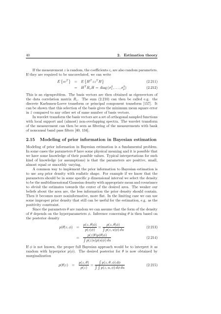
40 2. Estimation theory
If the measurement z is random, the coefficients c i are also random parameters.
If they are required to be uncorrelated, we can write
E { cc T } = E { H T zz T H } (2.211)
= H T R z H = diag (σ 2 1,...,σ 2 p) (2.212)
This is an eigenproblem. The basis vectors are then obtained as eigenvectors of
the data correlation matrix R z . The sum (2.210) can then be called e.g. the
discrete Karhunen-Loeve transform or principal component transform [157]. It
can be shown that this selection of the basis gives the minimum mean square error
in ẑ compared to any other set of same number of basis vectors.
In wavelet transform the basis vectors are a set of orthogonal sampled functions
with local support and (almost) non-overlapping spectra. The wavelet transform
of the measurement can then be seen as filtering of the measurements with bank
of noncausal band pass filters [40, 134].
2.15 Modeling of prior information in Bayesian estimation
Modeling of prior information in Bayesian estimation is a fundamental problem.
In some cases the parameters θ have some physical meaning and it is possible that
we have some knowledge of their possible values. Typical interpretations for such
kind of knowledge (or assumptions) is that the parameters are positive, small,
almost equal or smoothly varying.
A common way to implement the prior information to Bayesian estimation is
to use any prior density with realistic shape. For example if we know that the
parameters should be in some specific p dimensional interval we select the density
to be the multidimensional Gaussian density with appropriate mean and covariance
to shrink the estimates towards the center of the desired area. The weaker our
beliefs about the area are, the less information the prior density should contain.
Then it becomes more noninformative, more flat. In the limiting case we can use
some improper prior density that still can be useful for the estimation, e.g. as the
positivity constraint.
Since the parameters θ are random we can assume that the form of the density
of θ depends on the hyperparameters φ. Inference concerning θ is then based on
the posterior density
p(θ|z,φ) = p(z,θ|φ)
p(z|φ)
=
= ∫ p(z,θ|φ)
(2.213)
p(z,u|φ)du
p(z|θ)p(θ|φ)
∫
p(z|u)p(u|φ)du
(2.214)
If φ is not known, the proper full Bayesian approach would be to interpret it as
random with hyperprior p(φ). The desired posterior for θ is now obtained by
marginalization
p(θ|z) = p(z,θ)
p(z)
=
∫
p(z,θ,φ)dφ
∫ ∫
p(z,u,φ)dφdu
(2.215)