Supplementary Handout for ME 147 Mechanical Vibrations Fall ...

Supplementary Handout for ME 147
Mechanical Vibrations
Fall 2001
Instructor: Faryar Jabbari
Department of Mechanical Engineering
University of California, Irvine
0–1

1 Preliminaries and Background Material
Imaginary
P
b
A
O
θ
a
Figure 1: A vector in the complex plane
Real
1.1 Complex Numbers, Polar coordinates
Recall that we define
i = √ −1 (sometimes we use ‘j ′ !) (1.1)
Now in the diagram above, consider point ‘P’ in the complex plane. We denote the
length OP = A, where clearly,
a = Acosθ, b = Asinθ (1.2)
We can use one of the following coordinates
Cartesian Coordinates : P = a + ib (1.3)
P olar Coordinate : P = Ae iθ (1.4)
1–2

Equations (1.2)-(1.4) imply e iθ = cosθ +jsinθ, which is the same as the Euler’s’ identity
further below. We can use these equations to do basic operations on complex numbers
Addition: let
X 1 = A 1 e iwt , X 2 = A 2 e i(wt+φ)
where φ is the phase angle between the X 1 and X 2 .Then
X 1 + X 2 =(A 1 + A 2 e iφ )e iwt =[(A 1 + A 2 cosφ)+iA 2 sinφ]e iwt = A 3 e i(wt+α)
where
A 2 3 =(A 1 + A 2 cosφ) 2 +(A 2 sinφ) 2
and
tanα =
A 2 sinφ
A 1 + A 2 cosφ
Multiplication: let
X 1 = A 1 e iθ 1
, X 2 = A 2 e iθ 2
then
X 1 X 2 = A 1 A 2 e i(θ 1+θ 2 )
Why Can you show it
Square root, etc.: From multiplication, we know that
(Ae iθ )(Ae iθ )=A 2 e i2θ
therefore, we can write
(Ae iθ ) n = A n e inθ
where n can be any real number (and not necessarily an integer). For example,
(Ae iθ ) 1 2 = A 1 2 e i θ 2
1–3

or more generally
(Ae iθ ) 1 n = A
1
n e
i θ n
Derivatives: Now suppose that θ was changing with a constant rate of change, i.e., θ = wt
for some w, and point P , as a result, is rotating counter clockwise.
Then vector P is
changing with time, therefore, it has time derivative (or velocity!), i.e.,
P = Ae iwt (1.5)
Ṗ = iwAe iwt = iwP (1.6)
¨P = −w 2 Ae iwt = −w 2 P (1.7)
Finally, think about taking derivative of ‘a ′ in (1.2). We can write
ȧ = −wAsinθ, ä = −w 2 cosθ (1.8)
or we can use the following
a = Real(P )=Real(Ae iwt )
and therefore,
and similarly
ȧ = Real(Ṗ )=Real(iwP )=−wAsinθ (1.9)
ä = Real( ¨P )=Real(−w 2 P )=−w 2 Acosθ (1.10)
We will see in future chapters that this trick can save a great deal of time.
1–4

1.2 Power Series, etc
1.3 Euler’s Identity, . . .
e x =
∞∑
k=0
cos θ =1− θ2
2! + θ4
4!
sin θ = θ − θ3
3! + θ5
5!
x k
k!
(1.11)
for θ real (1.12)
for θ real (1.13)
e iθ =cosθ + i sin θ (1.14)
e −iθ =cosθ − i sin θ (1.15)
cos θ = eiθ + e −iθ
2
(1.16)
sin θ = eiθ − e −iθ
= −i(eiθ − e −iθ )
2i
2
(1.17)
1.4 Trigonometric Identities
(A + B) (A − B)
sin A +sinB =2sin cos
2 2
(1.18)
(A + B) (A − B)
cos A +cosB =2cos cos
2 2
(1.19)
sin(A + B) =sinA cos B +sinB cos A (1.20)
cos(A + B) =cosA cos B − sin A sin B (1.21)
sin A sin B = 1 [− cos(A + B)+cos(A − B)]
2
(1.22)
cos A cos B = 1 [cos(A + B)+cos(A − B)]
2
(1.23)
sin A cos B = 1 [sin(A + B)+sin(A − B)]
2
(1.24)
1–5

1.5 Orthogonality Conditions for Fourier Series
Let w = 2π
τ
, where τ is in seconds (i.e., period of motion), then for all positive integers n
and m following identities hold:
∫ τ/2
−τ/2
∫ τ/2
−τ/2
∫ τ/2
−τ/2
∫ π
{
0 if m ≠ n
cos nwt cos mwt dt = τ
2
if m = n
{
0 if m ≠ n
sin nwt sin mwt dt = τ
2
if m = n
{
0 if m ≠ n
cos nwt sin mwt dt =
0 if m = n
{
e inx e −imx 0 if m ≠ n
dx =
2π if m = n
−π
(1.25)
(1.26)
(1.27)
(1.28)
1–6

2 Fourier Series
Consider a periodic function x(t) withaperiodofτ ; i.e.,
We define the following :
x(t) =x(t + τ) =x(t +2τ) =.... for all t.
w 1 = 2π
τ
fundamental frquency or ‘harmonic ′
w n = nw 1 , n =2, 3, 4,... higher harmonics
The basic idea is that the periodic function, x(t), can be represented by a, possibly
infinite, sum of its harmonics (i.e., its ‘Fourier Series Representation’):
x(t) = a o
2
+ a 1 cos w 1 t + a 2 cos w 2 t + a 3 cos w 3 t + ··· (2.1)
+ b 1 sin w 1 t + b 2 sin w 2 t + b 3 sin w 3 t + ··· (2.2)
Finding a i ’s and b i ’s (which are called the Fourier coefficients) is relatively simple. For
example, multiply (2.1) by cosw n t, integrate both sides and use the orthogonality conditions
(from the previous section) to get the following
a n = 2 τ
∫ τ
2
− τ 2
x(t) cos w n tdt ,w n = nw 1 , n =1, 2, 3,... (2.3)
b n = 2 τ
∫ τ
2
− τ 2
x(t) sin w n tdt ,w n = nw 1 , n =1, 2, 3,... (2.4)
a o = 2 τ
∫ τ
2
− τ 2
x(t)dt i.e., the average
2–1

Next, recall that
AcosX + BsinX = √ A 2 + B 2 cos (X − φ) (2.5)
= √ A 2 + B 2 sin (X − φ)
where
tan φ = B A
Therefore, we can rewrite the Fourier series representation as
x(t) = a o
2 + ∞ ∑
2.1 Complex Representation
n=1
c n = √ A 2 + B 2 , tan φ = b n
a n
c n cos(w n t − φ n ), (2.6)
We can also use Euler’s identity to provide another form of the Fourier series. Using the
(complex) exponential form of cos and sin (e.g., cos x = eix +e −ix
2
), we can rewrite (2.1) as
x(t) = a o
2 + ∞ ∑
n=1
= a o
2 + ∞ ∑
n=1
recalling w n = nw 1 ,wecanwrite
x(t) =
∞∑
n=−∞
c n e inw 1t
[ a n
e iwnt + e −iwnt
2
e iwnt ( a n
2 + b n
2i ) + ∞ ∑
, where
⎧
⎪⎨
⎪⎩
+ b n
e iwnt − e −iwnt
2i
n=1
e −iwnt ( a n
2 − b n
2i )
c o = ao
2
c n = an−ibn
2
, n > 0
c n = an+ibn
2
, n < 0
We can simplify a bit more. For example, consider the expression for c n for n>0: using
the definitions of a n and b n from (2.3) and (2.4), respectively, we get
]
c n = 1 2 (a n − ib n )= 1 2 { 2 τ
∫ τ
2
− τ 2
(x(t)cosnw 1 n − ix(t)sinnw 1 t) dt }
2–2

or
c n = 1 τ
∫ τ
2
x(t)(cos nw 1 n − i sin nw 1 t) dt = 1 τ
∫ τ
2
x(t)e −inwnt dt
− τ 2
− τ 2
Similarly, for n

3 Notes for Chapter 3
3.1 Frequency Response
Consider the differential equation,
mẍ + cẋ + kx = F (t) =F o cos wt. (3.1)
After taking the Laplace transform, we get
x(s) =
msx(0) + mẋ(0) + cx(0)
ms 2 + cs + k
+
F (s)
ms 2 + cs + k = x 1(s)+x 2 (s) (3.2)
where F (s) is the Laplace transform of F (t), i.e.,
F (s) =
With these, we make the following definition
Definition: Set x(0) = ẋ(0) = 0.
F os
s 2 + w 2
Transfer Function △ = H(s) = x(s)
F (s) = 1
ms 2 + cs + k
(3.3)
i.e., the transfer function is the ratio of the output (i.e., x) to the input (i.e., F )inthe
s-domain, setting all initial condition to zero. Now, going back to (3.2), and taking inverse
Laplace, we have
x(t) =x 1 (t)+x 2 (t).
Consider the first term. From the results of chapter 2, we know that
x 1 (t) =e −ζwnt (X 1 cosw d t + X 2 sinw d t)
√
where X 1 and X 2 depend on the initial conditions and w d = w n 1 − ζ 2 . Aslongaswe
have some damping, the exponential terms decays to zero; i.e., x 1 (t) → 0ast →∞. As a
result,
x steadtstate (t) =x ss (t) =x 2 (t).
3–1

From now on, let us focus on this steady state solutions (i.e., we either have no initial
conditions or we assume that the transients die out fast and we need to study long term
behavior). We will try the odd ‘partial fraction expansion’ method
x 2 (s) =H(s) F (s) =
1
ms 2 + cs + k
F o s
s 2 + w 2 = As + B
s 2 + w 2 +
Ds + C
ms 2 + cs + k
(3.4)
Ds+C
where A, B, C and D are to be found. Now the last term (i.e.,
ms 2 +cs+k
) results (after
inverse Laplace transform) in terms like e −ζwnt (....), just as in x 1 (t), which goes to zero as
time goes to infinity. Therefore, for the steady state response, we can concentrate on the
term As+B
s 2 +w 2 . For this, multiply (3.4) by s 2 + w 2 to get
H(s)F o s =(As + B)+H(s)(Ds + c)(s 2 + w 2 ). (3.5)
This equation is true for all values of s. In particular, we can use two specific values
that let the last term disappear; i.e, s = ±iw! toget
H(iw)F o iw = Awi + B (3.6)
−H(−iw)F o iw = −Awi + B (3.7)
Solving these two equations (by adding and subtracting them from each other) yields
{
B =
1
2 F owi [H(iw) − H(−iw)]
A = 1 2 F o [H(iw)+H(−iw)]
(3.8)
Since the rest of the coefficients of H(s) are real, we have H(−iw) =H(iw) which
results in
{
A = Fo Real[H(iw)]
B = −F o wImag[H(iw)]
As a result, using (3.8) in (3.4), after a little bit of work, we have
(3.9)
x ss (s) =F o Real[H(iw)]
s
s 2 + w 2 − F w
oImag[H(iw)]
s 2 + w 2 (3.10)
3–2

or, after taking the inverse Laplace
using the trig. identity
x ss (t) =F o Real[H(iw)] cos wt − F o Imag[H(iw)] sin wt (3.11)
AcosX − BsinX = √ A 2 + B 2 cos(X + φ),
tanφ = B A
we get {
xss (t) =|H(iw)| F o cos(wt + φ)
tanφ = Imag[H(iw)]
Real[H(iw)]
where |H(iw)| is called the ‘gain’ and φ is the phase of the transfer function H(s).
(3.12)
NOTE: H(s) can be more general, i.e., larger than second order. The algebra would be
somewhat more complicated, but the same result, i.e., (3.12).
SUMMARY: When the input (i.e., the forcing function) for the (3.1) is a simple sine (or
cosine), the steady state response is a sine (or cosine), at the same frequency. The magnitude
of the response is the magnitude of the forcing function multiplies by the magnitude of the
transfer function of the system at the frequency of the forcing function (i.e., |H(iw)|). The
response will also have a phase difference with the input (which is equal of the angle of
H(iw)). The process can be seem below.
Step 1 : Write the differential equation of motion
Step 2 : Take Laplace Transform
Step 3 : Set initial conditions to zero and find H(s) inx(s) =H(s)F (s), where F (s) is
the Laplace transform of the forcing function.
Step 4 : The steady state gain - magnification - from input to output is |H(iw)| and the
phase is φ as define above. (w is the frequency of the forcing function)
3–3

4 A Brief Review of Chapter 4
We start with
mẍ + cẋ + kx = F (t) (4.1)
In chapter 2, we set the forcing function to be zero, while in chapter 3 we solved the
problem when the forcing function was a simple sine or cosine. Here, we study the case
where F (t) has more complicated forms.
4.1 A: F (t) is periodic
When the forcing function is periodic; i.e., F (t) =F (t + τ) =F (t +2τ) ... for some fixed
period τ, we can use the Fourier series results we studied in Chapter 1. Recall that we can
‘break’ down a nasty looking periodic function as a sum of a sines and cosines; i.e.,
F (t) = a o
+ a 1 coswt + b 1 sinwt + a 2 cos2wt + b 2 sin2wt + ···
2
= f 1 (t)+f 2 (t) +f 3 (t) +f 4 (t) +f 5 (t) +··· (4.2)
Equation (4.1) thus becomes
mẍ + cẋ + kx = f 1 (t)+f 2 (t) +f 3 (t) +f 4 (t) +f 5 (t) +··· (4.3)
Next, recall from your differential equation course (M3D, for example) that we can use
the ‘superposition’ technique for a linear differential equation. That is, we solve (4.1) as
if f i (t) is the only forcing function and call the solution to it x i (t).
Repeating this for
i =1, 2, ... the solution to the actual problem is
x(t) =x 1 (t)+x 2 (t) +x 3 (t) +x 4 (t) +x 5 (t) (4.4)
4–1

where the x i (t)’s satisfy
⎧
⎪⎨
⎪⎩
mẍ 1 + cẋ 1 + kx 1 = f 1 (t) = ao
2
mẍ 2 + cẋ 2 + kx 2 = f 2 (t) =a 1 cos wt
mẍ 3 + cẋ 3 + kx 3 = f 3 (t) =b 1 sin wt
.
.
.
.
.
(4.5)
Each of the equations in (4.5) was solved in chapter 3. See the text book (page 265, equation
4.13) for the complete solution (with all of the bells and whistles). We can summarize
as
Summary:
• Break down the periodic forcing function, F (t), into its harmonic components via the
Fourier series.
• Solve the simple equations in (4.5) (each with a single harmonic forcing function) and
solve for x i (t).
• Add all of these x i (t) together to get the whole solution.
4.2 F (t) is not periodic, but F (s) is obtainable
Next, we consider the forcing functions that are not necessarily periodic (they could be!)
and we assume that we can find the Laplace transform of the forcing function; i.e, F (s)
is known.
In this case, we simply take the Laplace transform of the equation, find the
expression for x(s) and then take the inverse Laplace transform to get x(t). That is , first
we take the transform of (4.1) to get
(ms 2 + cs + k)x(s) =F (s)+msx(0) + mẋ(0) + cx(0)
4–2

where F (s) is the Laplace transform of F (t). Now we have
x(s) =
1
+ mẋ(0) + cx(0)
ms 2 F (s)+msx(0)
+ cs + k ms 2 = H(s)F (s)+H(s)[msx(0)+mẋ(0)+cx(0)]
+ cs + k
(4.6)
wherewehaveusedH(s) (i.e., the transfer function) as defined in the previous chapter.
Next, we just go ahead and take the inverse Laplace of x(s); i.e.,
x(t) =L −1 [x(s)] (4.7)
If you were interested in only the steady state solution, you would ignore the second
term (or set the initial conditions to zero). The only problem is that this can end up being
very messy and tedious and is probably useful for a ‘simple’ forcing functions.
4.3 General Forcing Function
Now let us consider the most general case: While F (s) may exist, either we can not find or
calculate F (s) or it is very tedious and hard to do so. We go back to the previous subsection.
For a moment assume that we had F (s), recall from (4.6) that
x(s) =
1
ms 2 + cs + k F (s)+ = H(s)F (s)+H(s)[msx(0)+mẋ(0)+cx(0)] = H(s)F (s)+x T (s)
whereweusex T to denote the component of x that is ‘transient’ and does not play a role
in steady state (and is the exponentially decaying functions we saw in Chapter 2). Now,
after taking the inverse Laplace transform of this equation, we have
x(t) =x T (t)+L −1 [H(s)F (s)] (4.8)
where x T (t) is exponentially decaying part. So, we focus on the second part of x(t). Now
recall the ‘convolution’ property of the Laplace transform (see Section 4.7 of the test, for
example) which says
∫ t
L [ f 1 (t − τ)f 2 (τ)dτ] =F 1 (s) F 2 (s) (4.9)
0
4–3

or equivalently
∫ t
L −1 [ F 1 (s) F 2 (s)] [ f 1 (t − τ)f 2 (τ) dτ
0
where F 1 (s) andF 2 (s) are the Laplace transforms of f 1 (t) andf 2 (t), respectively. Now
comparing (4.8) and (4.9), we can write
∫ t
∫ t
x(t) =x T (t)+ h(t − τ)F (τ)dτ = x T (t)+ F (t − τ)h(τ)dτ (4.10)
0
0
(make sure you can show the two integrals in the last equation are equal to one another).
Here we have used the following definitions
F (t) =L −1 [F (s)],
the forcing function
h(t) =L −1 [H(s)], the Impulse Response (4.11)
Now, equation (4.10) can be computed numerically if one has data for F (t) (forexample,
records of wind gusts or ground motion during an earthquake) and does hot have to be done
analytically.
The last remaining question is regarding the h(t) - which was defined in (4.11) as the
inverse Laplace of the Transfer Function H(s). In our problem, we have
H(s) =
1
1
ms 2 + cs + k = m
s 2 + c m s + k m
=
1
m
s 2 +2ζw n s + w 2 n
using the definitions we used for ζ and w n in chapters 2 and 3 (i.e., w 2 n = k m and c m =2ζw n).
Next, using the Laplace transforms table (e.g., the one in the back of the text), we have
h(t) = 1
mw d
e −ζwnt sin w d t w d = w n
√
1 − ζ 2 (4.12)
4–4

4.4 Closing Remarks
1. h(t) is called the ‘impulse response’ of the system because it is the response - or
reaction - of the system (i.e., the mass spring dashpot system) to an ‘impulsive’ force
of unit intensity. A unit impulse force is a large sudden force that is applied for a very
short duration (such that the integral ∫ Fdt=1).
2. You can also get h(t) if you release the system with x(0) = 0 but ẋ(0) = 1 m . The
resulting x(t) would be exactly the same as h(t) in (4.1) - see text for details.
3. Algorithm: The approach in this subsection can be considered as following this algorithm:
• get F (t), either in closed form or by data
• find h(t), basically from (4.11) or (4.12)
• Calculate the integral, either analytically (by hand or Mathematica, etc) or numerically.
4. The approach here applies to more general systems. Systems with more degrees of
freedom (e.g, more than one mass), systems with more forcing functions, etc. All that
is required is F (t) andtheh(t).
4–5

5 Notes for Chapter 5
5.1 A Brief Review of Linear Algebra
Consider the systems of equations
{
a11 x 1 + a 12 x 2 =0
a 12 x 1 + a 22 x 2 =0
(5.1)
where a 11 ,a 12 ,a 21 and a 22 are known constants. We can write this set of equations in
the matrix form
Ax =0
where
A =
[ ]
a11 a 12
a 12 a 22
, x =
[
x1
x 2
]
, 0 =
[
0
0
]
Now, we recall the following from linear algebra
• If det[A] ≠0,thenA −1 exists, and therefore,
Ax =0 , ⇒ A −1 Ax =0 ⇒ x =0
Now, if we hope to find nontrivial (i.e., non zero) solutions to this equation, we need
to avoid what just happened, i.e., we need to avoid det[A] ≠0!
• det[A] ( ) = 0, then there exits ((many) ) ( solutions ) to the ( equation. ) For example, if x =
1 2 0.1
1
is a solution, so are , ,andα for any α (why)
2
4 0.2
2
Now, recall that if det[A] = 0 then the two equations in (5.1) are not independent. In
short, there is really one equation and two unknowns. Therefore, you cannot solve for both
5–1

of the unknowns. The best you can do is to express one of the unknowns in terms of the
other one. For example,
x 1 = − a 12
a 11
x 2 or x 2 = − a 11
a 12
x 1
so if you knew either x 1 or x 2 , you could find the other one. As a result, the solutions are
of the form (
) ( )
x 1
1
− a =
11
a 12
x 1 − a 11
a 12
x 1
or equivalently, ( )
−
a 12
a 11
x 2
=
x 2
(
−
a 12
a 11
1
)
x 2 .
5.2 Back to Chapter 5
Suppose that free vibration of a system is modeled by the following differential equations
Mẍ(t)+Kx(t) = 0 (5.2)
where M and K are the mass and stiffness matrices 2 × 2, respectively, and x(t) isa2× 1
vector.
Parallel to the single degree of freedom, we make the following assumption regarding
the form of the solution for (5.2) (an assumption that is verified and motivated by Laplcace
Transfomrs - believe it or not)
x(t) =X cos (wt + φ) { or X sin (wt + φ) } (5.3)
We need to find w and φ. Use (5.3) and plug in (5.2) to get
−w 2 MX cos (wt+φ)+KX cos (wt+φ) =0
⇒ (K −w 2 M)X cos (wt+φ) =0 ,forallt.
Since cos (wt + φ) is not zero all the time, (and K − w 2 M is constant) we must have
(K − w 2 M) X =0 (5.4)
5–2

Now, X is the magnitude of the motion (recall (5.3)), so we are only interested in nonzero
X. Remembering the results from the previous section, the problem has non-zero solution
if
det[K − w 2 M]=0
which is a determinant of a 2 × 2 matrix. Now if you remember how to take determinants
(BIG IF!), you would notice that the determinant will have constants, powers of w 2 and w 4
only (think about this a bit). So it is a second order equation in terms of w 2 and we can
solve it rather easily; i.e.,
det[K − w 2 M]=0⇒ 2 values for w 2 : w 2 1 , w2 2
We will see later (in Chapter 6) that the values one gets for w 2 1 and w2 2
will always be
either positive or zero. Now each w i corresponds to a value of w for which det(K − w 2 M)
becomes zero. Therefore, for these values of w only, we can find nonzero vectors X. Since
we have two potential value for w, we write the solution as
x(t) =X (1) cos (w 1 t + φ 1 )+X (2) cos (w 2 t + φ 2 ) (5.5)
Note the similarity between the general form of the solution for the 2-degree-of freedom
system and that of the 1-degree of freesdom system we saw in Chapter 2.
Now let us go back to (5.4). We have two values for w that make the determinant zero
(and for other values of w this determinant is not zero). For example, for w 1 ,wehavethe
determinant zero and thus we can have a nontrivial (i.e., nonzero) solution to (5.4), i.e., we
can hope to solve for
(K − Mw1)X 2 (1) =0
where X (1) is the X solution in (5.4) that corresponds to w 1 . From the review material, we
5–3

know that we cannot solve for X completely, but we can get an answer of the form
[
X (1) X (1) ] [ ]
=
1
r (1) X (1) = X (1) 1
1
r (1) 1
(5.6)
Where X (1)
1 is unknown, but r (1) depends on the entries of K and M and can be
calculated easily.
Similarly, we can start with w 2 and solve the corresponding X in the
form
X (2) =
[
X (2)
1
r (2) X (2)
1
]
= X (2)
1
[
1
r (2) ]
Using these last two expressions, we get the following form for the general solution
x(t) =X (1)
1
[
1
r (1) ]
cos (w 1 t + φ 1 )+X (2)
1
[
1
r (2) ]
(5.7)
cos (w 2 t + φ 2 ) (5.8)
static equilibrium line
K1
l1
e
c.g.
o
l2
θ
x
K2
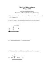
Figure 2: A two degree of freedom system
NOTES:
5–4

• Note that there are four unknowns in the general solution (the two φ i and the two
X (i) ). See equations 5.17 and 5.18 of the text for explicit formulas that can be used
to obtain these unknowns, given the initial positions and velocities.
• w 1 and w 2 are called the natural frequencies of the system. They depend on K
and M only and not the initial conditions. Also, judging from the general solution,
once the system is released from a set of initial conditions, the motion ensuing motion
is either a periodic motion with w 1 or w 2 (or a combination of the two frequencies).
[ ] [ ]
1
1
• The vectors
r (1) and
r (2) are also independent of intial condition and only
depend on the K and M matrices. [ ] These vectors are called the modes shapes of
1
the system. For example,
r (1) is the mode shape corresponding to the natualr
frequency w 1 . This mode shape, then shows the ‘form’ or ‘shape’ of the motion of
the system if the motion was comprised of w 1 term only. Indeed, there are initial
conditions that would result in a motion that has a single [ frequency ] of w 1 where the
1
ration of the motion of x 1 to x 2 is r (1) - i.e., the vector
r (1) shows the ‘shape’ of
the motion.
5.3 An important example (page 344 of the text)
Consider the system in the Figure 2 (also see Figure 5.10 on page 344 of the text!). Let
x(t)
: Motion of center of gravity from the equilibrium position(positive is down)
θ = rotation of the bar (positive direction is clockwise)
The equation of motion can be written as
mẍ = −(x + l 2 sinθ)k 2 − (x − l 1 sinθ)k 1
5–5

J ¨θ = −(x + l 2 sinθ)k 2 l 2 +(x − l 1 sinθ)k 1 l 1
Now linearize the equaitons (i.e., sinθ = θ, cosθ =1, θsinθ =0, etc) and put them
in the matrix form, you will get
[
m 0
0 J
]{
ẍ
¨θ
}
+
[
k 1 + k 2 −(k 1 l 1 − k 2 l 2 )
−(k 1 l 1 − k 2 l 2 ) k 1 l1 2 + k 2l2
2
]{
x
θ
} {
0
=
0
}
(5.9)
or in short hand
Mẍ + Kx =0
with obvious definitions for K, M, etc. Next, let us see what happens if we wanted to write
the equations of motion in terms of y(t), the motion of a point e units to the left of the
center of gravity First, note that
y = x − esinθ ⇒ ẏ =ẋ − e ˙θcosθ
ÿ =ẍ − e¨θcosθ + e ˙θ 2 sinθ
which after linearization, becomes y = x − eθ and ÿ =ẍ − e¨θ, or
{ } [ ]{ } { } [
y 1 −e x ÿ 1 −e
=
, =
θ 0 1 θ ¨θ 0 1
]{
ẍ
¨θ
}
(5.10)
Now we define
and using (5.10), we get
{
ẍ
¨θ
T =
}
=
[
1 −e
0 1
[
1 e
0 1
] −1
=
]{
ÿ
¨θ
[
1 e
0 1
}
= T
]
{
ÿ
¨θ
}
(5.11)
(5.12)
Using this last expression in (5.9), the matrix form of the equations (in terms of y and
θ) becomes
MT
{
ÿ
¨θ
}
+ KT
{
y
θ
}
=0
5–6

premultipyling by T T ,
T T MT
{
ÿ
¨θ
}
+ T T KT
{
y
θ
}
=0
where we can write in short hand as
ˆM
{
ÿ
¨θ
}
+ ˆK
{
y
θ
}
(5.13)
where both
ˆM and ˆK are symmetric, if the original K and M were symmetric and after
some algebra
[
ˆK = T T KT =
[ ]
ˆM = T T m me
MT =
me J
]
k 1 + k 2 k 2 (l 2 + e) − k 1 (l 1 − e)
k 2 (l 2 + e) − k 1 (l 1 − e) k 1 (l 1 − e) 2 + k 2 (l 2 + e) 2
Remark: Note that instead of writing the equations of motion in terms of y, wewrite
the more natural form (i.e., in terms of x), and use the ‘transformation’ of (5.12) to relate
the original coordiantes to the desired coordinate. We have thus used a ‘coordinate
transformation’.
What if someone asked you for the equations of motion in terms of the motion of the
ends of the rod (let us call them x 1 and x 2 ) We follow the procedure we used above in the
change of coordinates.
x 1 = x − l 1 sinθ ,
x 2 = x + l 2 sinθ
which after linearization, becomes
{ } [ ]{
x1 1 −l1 x
=
x 2 1 l 2 θ
}
(5.14)
Similarly, taking two derivatives of the x 1 equation above, for example, one gets
ẍ 1 =ẍ − l 1 ¨θcosθ + l1 ˙θ2 sinθ
5–7

linearizing and combing with the ẍ 2 equation, we get
{ } [ ]{
ẍ1 1 −l1 ẍ
=
ẍ 2 1 l 2
¨θ
}
Now we define
˜T =
[ ] −1
1 −l1
= 1
[
l2 l 1
1 l 2 l 1 + l 2 −1 1
]
(5.15)
as a result, we can write
{
ẍ
¨θ
}
= ˜T
{
ẍ1
ẍ 2
}
(5.16)
with a similar form for the x and θ. Using this last expression in (5.9), and post multiplying
by ˜T (exactly as the previous example) the equations of motion become
{ } ( )
˜T T M ˜T
ẍ1
+
ẍ ˜T T K ˜T
x1
=0
2 x 2
or in compact form
( ) ( )
ẍ1
˜M +
ẍ ˜K
x1
=0
2 x 2
where, for example,
˜M = ˜T T M ˜T =
[ ]
1 J + ml
2
2 ml 1 l 2 − J
(l 1 + l 2 ) 2 ml 1 l 2 − J ml1 2 + J .
Questions: Think about the following questions
• Is one set of coordinates ‘better’ than others
• Are the natuaral frequencies one gets in the three difference sets of K and M the
same
• Are the mode shapes one gets in the three difference sets of K and M the same
5–8

k
m
F (t)= F_1 cos wt
x_1 (t)
k
m
x_2 (t)
k
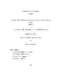
Figure 3: A simple two degree of freedom forced system
5.4 Forced Vibration
Consider the system of Figure 3 (or Figure 5.13 of text on page 351). This is a relatively
general two degrees of freedom system, in which some of the parameters are set equal to
one another to simpily the analysis.
Following regular procedure, the equation of motion are
Mẍ + Kx = F (5.17)
where
M =
[
m 0
0 m
]
[
2k −k
, K =
−k 2k
]
[
F1 cos wt
, F =
0
]
where x 1 (t) andx 2 (t) are the absolute displacments of the masses and w is the frequency
of the external forcing function. Parallel to the development of Chapter 3, we assume the
solution has the following form
x(t) =
[
x1 (t)
x 2 (t)
]
=
[
X1 coswt
X 2 coswt
] [ ]
X1
=
X 2
coswt = X coswt (5.18)
5–9

Plugging this in the equation of motion, (5.17), we get
[ ]
[
[K − Mw 2 F1
]X = ⇒ X =[K − Mw 2 ] −1 F1
0
0
]
so that (if the inverse exists) the motion becomes
x(t) =[K − Mw 2 ] −1 [
F1
0
]
coswt.
For 2 × 2 systems, it is possible to carry out the inverse analytically. Noting that
[K−Mw 2 ] −1 =
we get
[
2k − mw
2
−k
−k 2k − mw 2 ] −1
=
x(t) =
[
x1 (t)
x 2 (t)
]
⎡
= ⎣
1
(3k − mw 2 )(k − mw 2 )
F 1 (2k−mw 2 )
(3k−mw 2 )(k−mw 2 )
F 1 k
(3k−mw 2 )(k−mw 2 )
[ ]
2k − mw
2
k
k 2k − mw 2
⎤
⎦ coswt (5.19)
The (normalized) magnitude of each x i (t) asw changes is shown on the plots shown on
pages 352 of the text. Note some very interesting properties:
• As w 2 gets closer to either k m or 3k m
the amplitude of both masses gets very large;
i.e, we observe the ‘resonance’ behavior. Recall that for this problem, the natural
frequencies are exactly
√ k
m and √ 3k
m
• We have ignored damping because (as you might have expected from the one degree of
freedom case!) it makes the problem much much more complicated - without adding
new insight. The peaks will be finite and valleys will be shallower of course. We will
deal damping in some detail in Chapter 6.
• In the motion of x 1 (t), see what happens as w 2 gets close to 2k m
Note that while
x 2 (t) ≠ 0, we will get x 1 (t) = 0!!
This value also depends on mass and stiffness
properties of the system. If this condition holds, the system behaves as a ‘vibration
absorber’. That is, the second mass ‘absorbs’ the vibration that the forcing function
5–10

might create and allows the first mass to stay stationary. We will study this in more
detail in Chapter 9.
• In the language of controls (ME170B), 2k m
is the zero for the transfer function from F
to x 1 (and the natural frequencies are poles)
5–11

6 Multi-degrees-of-freedom Systems
6.1 Background
First, we start by writing the equations of motion
Mẍ(t)+Kx(t) =F (t) with no damping (6.1)
Mẍ(t)+Cẋ(t)+Kx(t) =F (t) with damping (6.2)
To do this, three different approaches can be used :
a. Directly from Newton’s laws
b. By inspection (via Section 6.4 of the book)
c. From the energy expressions (Section 6.5 of the book). For this approach, first note that
T = total kinetic energy = 1 2ẋT Mẋ
U = total potential energy = 1 2 xT Kx.
If you can shape the energy expression into the form on the right hand side, you have
obtained the M and K matrices.
From now on, we will assume (without any loss of
generality) that both M and K are symmetric.
Next, let us analyze the fundamental properties of the system. We will consider the
undamped and free vibration, for the moment.
6.2 Undamped, free vibration
Mẍ(t)+Kx(t) = 0 (6.3)
Similar to development of Section 6.9 of the book, and consistent with what we did for
the one and two degrees of freedom systems, we search for motions of form x(t) =Xcoswt,
6–1

where x(t) is the vector of the coordinates we have used (for example, displacements of each
degree of freedom). We get
[−w 2 M + k]X =0 (6.4)
where non-trivial solution can be found ONLY IF det[−w 2 M + k] = 0.
So we set this
determinant to zero and find the values of w that result in this determinant becoming zero;
i.e.,
det [−w 2 M + K] =0 =⇒ w 1 , w 2 ···w n
where these w i ’s are called the natural frequencies (you will soon see why!) and are roots
of the determinant equation. It is relatively easy to show that this equation has n solutions
for w 2 . It is somewhat more difficult to show that all solutions are nonnegative (i.e., either
zero or positive numbers). For each w i , solve the following equation for X i
[−w 2 i M + K]X i =0.
As before, if X i satisfies this equation, so does aX i , for any scalar a. The pairs (w i ,X i )are
called the i th natural frequency and mode shape of the system. Note the similarity between
what we did here and the development of the two degree of freedom systems. The problem
is that for n ≥ 3, this process is not practical. Let us start by rewriting (6.4),
[−w 2 M + k]X =0=⇒ KX = w 2 MX or M −1 KX = w 2 X. (6.5)
The last 2 equations are two forms of the well known ‘eigenvalue’ problem, for which a
great deal of reliable, efficient and accessible software has been developed; i.e., in practice
we follow
(6.5) + computer programs =⇒ npairsof(wi 2 ,X i )
where wi 2,X i are called the i th eigenvalue and its corresponding eigenvector for (6.5), respectively.
6–2

The following properties of the eigenvalue problem are well known, and can be shown
through basic linear algebra:
• All n natural frequencies or eigenvalues of (6.5); i.e., w1 2,w2 2 ,...w2 n , are real and nonnegative.
• All n mode-shapes or eigenvectors of (6.5), X 1 ,X 2 ,...X n , corresponding to respective
w i ’s, are real and are linearly independent of one another.
Why are we interested in these For the following reasons
a. Physical understanding of the motion. Think of the vibrating string, for analogy. The
w i ′ s are similar to the ‘harmonics’ of the string, while the mode shapes are similar to the
shape corresponding to each harmonic (the half sine-waves in the vibrating string). They
give important information about resonance (more on this below) and the points where each
mode shape has maximum or minimum motion (for sensor/actuator placement, attachment
design, etc).
b. Damping analysis, uncoupling of the equation of motions, and order reduction: These
three are combined because they all follow from the orthogonality property of mode shapes
(or eigenvectors), see Section 6.10.2 of the text for details.
X T i MX j =0 if i ≠ j,and X T i MX i
△
= m i (6.6)
X T i KX j =0 if i ≠ j,and X T i KX i
△
= ki . (6.7)
These m i ’s and k i ’s are sometimes called generalized mass and stiffness of the i th coordinate.
Note that since we can have any value between 1 and n for i or j, equations (6.6) and
6–3

(6.7) represent n 2 equations, each. As an (easy) exercise, convince yourself that putting all
n 2 equations in a matrix form results in the following
[X 1 ···X n ] T M[X 1 ···X n ]=B T MB = diag[m i ] (6.8)
[X 1 ···X n ] T K[X 1 ···X n ]=B T MB = diag[k i ] (6.9)
wherewehaveusedB as a short hand for the matrix of mode shapes; i.e.,
B =[X 1 X 2 ···X n ]. (6.10)
In (6.8) and (6.9), diag[m i ] mean a diagonal matrix with m i as its (i, i) entry. Finally, let
us normalize the mode shapes according to
ˆX i = 1 √
mi
X i . (6.11)
Again, it is an easy exercise to show that
[ ˆX 1 ··· ˆX n ] T M[ ˆX 1 ··· ˆX n ]= ˆB T M ˆB = I (6.12)
while with little work, one can show
[ ˆX 1 ··· ˆX n ] T K[ ˆX 1 ··· ˆX n ]= ˆB T K ˆB = diag[ k i
m i
]=diag[w 2 i ] (6.13)
where w ′ i s are the natural frequencies! We have used ˆB as a short hand for the matrix of
normalized mode shapes; i.e.,
ˆB =[ˆX 1
ˆX2 ··· ˆX n ]. (6.14)
EXERCISE: Verify the second equality in (6.13).
SKETCH: Recall that for matrices A, B, C, wehavedet(ABC) =detA×detB ×detC. Now
by standard results from the eigenvalue problem, det ˆB ≠0. Setdet ˆB T [−w 2 M + K] ˆB =0
6–4

6.3 Forced Vibration
We go back to equation (6.1),
Mẍ(t)+Kx(t) =F (t) =F o coswt (or coswt ) (6.15)
From math, ME170 or early chapters of ME147, we expect that the steady state response
(i.e., particular solution) be of the form x(t) =Xcoswt. Here, w is the frequency of the
forcing function and is known (as compared to free vibration) and X is NOT the mode
shape, and simply is the amplitude of response. Substitute this solution in (6.15)
[−w 2 M + K]X = F o =⇒ X =[−w 2 M + K] −1 F o
ONLY IF THE INVERSE EXISTS, that is only if the determinant of the matrix is not
zero. But we know that at w = w i (i.e., any of the natural frequencies discussed above)
this determinant is zero. Therefore, these w i ′ s are frequencies that if the system is forced
at, problems can arise, i.e., at the very least we cannot use what we have learned above.
Further below, we will see that the response goes to infinity! (hence resonance and the
name ‘natural frequencies’). To clarify this, we will use the mode shapes.
Next, let us define the following coordinates
x(t) =[X 1 X 2 ···X n ] q(t) =Bq(t). (6.16)
Remember that x(t) was a vector of physically meaningful coordinates (e.g., displacement,
rotation or velocity of specific points of the system). Vector q(t), however, is vector
of coordinates q i (t), which in general are not physically meaningful. The best we can say
is that each q i (t) represents how much of the overall motion, at time t, is due to the mode
shape (and natural frequency) i.
6–5

Use (6.16) in (6.15) and premultiply (6.15) by B T , and using the identities in (6.8)-(6.10),
you will get
diag[m i ]¨q(t)+diag[k i ] q(t) =B T F o coswt, (or sin) (6.17)
i.e., n un-coupled equations of motion, which can be solved a lot easier (even by hand!).
Let us try to solve the problem , as usual we assume q(t) = Qcoswt and, after some
simplification, (make sure you see how the following equation is obtained)
(−w 2 m i + k i )Q i = X T i F o =⇒ Q i =
X T i F o
(−w 2 m i + k i )
(6.18)
Note that, according to (6.18), if w 2 gets close to k i
m i
for any i, the corresponding q i (t) goes
to infinity and, due to (6.16), so does x(t) (i.e., resonance !) The behavior of each q i (t),
with respect to the forcing frequency w is similar to the plots in Figures 3.3 and 3.11 of
the book. From (6.13), one can see that these resonance values are the same as the natural
frequencies of the system.
Lastly, if forcing frequency, w, is not at resonance values, (6.18) is used to calculate q(t).
From (6.16) then, we can find x(t). Notice that if w is close to any of the w i ’s, then the
corresponding Q i in (6.18) will be large. As a result if the forcing frequency is relatively
close to one of the modes, then that mode will have strong presence in the overall response
(see (6.16)). Sometimes, we use the following phrase: if w is close to w i , then the i th mode
will be highly excited.
6.4 Damped Vibration
In this case, we have the following for the equations of motion
Mẍ(t)+Cẋ(t)+Kx(t) =F (t) (6.19)
6–6

In general, little is known about the true nature of the damping in many important
applications.
If C matrix in (6.19) does not have any specific structure, the resulting
response can be quite complicated and hard to understand.
Suppose however, that the
following is true for some positive scalars α and β
C = αM + βK (6.20)
Using (6.16) and (6.20) in (6.19), and premultiplying (6.19) by B T , similar to (6.17)yields,
diag[m i ]¨q(t)+diag[αm i + βk i ] ˙q(t)+diag[k i ] q(t) =B T F o coswt (6.21)
which is n decoupled second order differential equations, each of the type
m¨z + cż + kz = f.
The behavior of each q i (t), with respect to the forcing frequency, is thus the same
as Figure 3.11 of the book. As a result, effective damping, exponential decay and other
similar properties can be estimated or approximated for the system. Note that this simple
transformation of the original coupled equations into n decoupled equations can be achieved
because the damping matrix is of the form in (6.20).
There are other variations of this method, including variations of (6.20), but the development
above captures the crucial aspects of it. In many cases, α and β are chosen for the
best fit in data collected in lab.
6.5 Modal Truncation
Think about a large order model (e.g., that of a wing of an aircraft, satellite or a tall
building). Say, 50 degrees of freedom. After some testing, it may be determined that the
loading is from very low frequencies, and thus only the first three (again as example) modes
6–7

are excited. Since the other 47 modes are not excited, ignoring them is not a bad idea (as a
first approximation). This can be done through the following : Start with the full equations
of motion (n = 50)
Mẍ(t)+Kx(t) =F.
Using (6.16), we write
x(t) =Bq(t) =X 1 q 1 (t)+···X 50 q 50 (t).
The truncated system is based on the first three modes only; i.e.,
x tr (t) =X 1 q 1 (t)+X 2 q 2 (t)+X 3 q 3 (t) =B tr q tr (t)
where B tr is the first three columns of B (a 50 × 3 matrix) and q tr =[q 1 q 2 q 3 ] T . The
reduced (or truncated) model will then be the following 3 × 3 matrix equation
B T tr MB tr ¨q tr (t)+B T tr CB tr ˙q tr (t)+B T tr KB tr q tr (t) =B T tr F.
6–8