Time-Based Sampling of Social Network Activity Graphs
Time-Based Sampling of Social Network Activity Graphs
Time-Based Sampling of Social Network Activity Graphs

You also want an ePaper? Increase the reach of your titles
YUMPU automatically turns print PDFs into web optimized ePapers that Google loves.
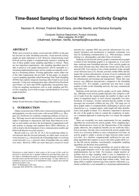
<strong>Time</strong>-<strong>Based</strong> <strong>Sampling</strong> <strong>of</strong> <strong>Social</strong> <strong>Network</strong> <strong>Activity</strong> <strong>Graphs</strong><br />
Nesreen K. Ahmed, Fredrick Berchmans, Jennifer Neville, and Ramana Kompella<br />
Computer Science Department, Purdue University<br />
West Lafayette, IN 47907<br />
{nkahmed, fjohnber, neville, kompella}@cs.purdue.edu<br />
ABSTRACT<br />
While most research in online social networks (OSNs) in the past<br />
has focused on static friendship networks, social network activity<br />
graphs are quite important as well. However, characterizing social<br />
network activity graphs is computationally intensive; reducing the<br />
size <strong>of</strong> these graphs using sampling algorithms is critical. There<br />
are two important requirements—the sampling algorithm must be<br />
able to preserve core graph characteristics and be amenable to a<br />
streaming implementation since activity graphs are naturally evolving<br />
in a streaming fashion. Existing approaches satisfy either one<br />
or the other requirement, but not both. In this paper, we propose<br />
a novel sampling algorithm called Streaming <strong>Time</strong> Node <strong>Sampling</strong><br />
(STNS) that exploits temporal clustering <strong>of</strong>ten found in real social<br />
networks. Using real communication data collected from Facebook<br />
and Twitter, we show that STNS significantly out-performs state<strong>of</strong>-the-art<br />
sampling mechanisms such as node sampling and Forest<br />
Fire sampling, across both averages and distributions <strong>of</strong> several<br />
graph properties.<br />
Keywords<br />
Online <strong>Social</strong> <strong>Network</strong>s, Graph <strong>Sampling</strong>, Link Analysis<br />
1. INTRODUCTION<br />
Online social networks (OSNs) have witnessed tremendous growth<br />
and popularity over the recent years, with several OSNs (e.g., Myspace<br />
[2], Facebook [1]) routinely comprising millions <strong>of</strong> users today.<br />
The huge success and increasing popularity <strong>of</strong> social networks<br />
makes it important to characterize and study their behavior in detail,<br />
as such studies can drive the development <strong>of</strong> appropriate tools<br />
and systems to manage and maintain these OSNs effectively, as<br />
well as lead to the development <strong>of</strong> new communication models and<br />
behavioral theories in social sciences.<br />
Recent work (e.g., [22, 20, 18, 16, 5, 6]) in analyzing online social<br />
network data has focused primarily on either static social network<br />
structure (e.g., a fixed network <strong>of</strong> friendship links) or evolving<br />
social networks (e.g., a network where friendship links are added<br />
over time). However, OSNs are more than just a record <strong>of</strong> social<br />
Permission to make digital or hard copies <strong>of</strong> all or part <strong>of</strong> this work for<br />
personal or classroom use is granted without fee provided that copies are<br />
not made or distributed for pr<strong>of</strong>it or commercial advantage and that copies<br />
bear this notice and the full citation on the first page. To copy otherwise, to<br />
republish, to post on servers or to redistribute to lists, requires prior specific<br />
permission and/or a fee.<br />
MLG ’10 Washington, DC USA<br />
Copyright 2010 ACM 978-1-4503-0214-2 ...$10.00.<br />
network ties—popular OSN sites provide infrastructure for community<br />
formation and mechanisms to maintain community over<br />
time by facilitating communication (e.g., Wall postings), content<br />
sharing (e.g., photographs), and other forms <strong>of</strong> activities.<br />
Studying social network activity graphs (communications graphs<br />
overlaid on the friendship graphs) is as important as, if not more<br />
than, studying static friendship networks. First, activity graphs are<br />
<strong>of</strong>ten more relevant since they reflect the current state <strong>of</strong> the social<br />
network [26]. User activity is also a better predictor <strong>of</strong> the strength<br />
<strong>of</strong> ties between users [13]. Second, activities within OSNs directly<br />
impact the systems infrastructure, in terms <strong>of</strong> server workloads and<br />
Internet traffic conditions; thus studying activity graphs is critical<br />
for infrastructure provisioning and management. Third, they may<br />
possess very different characteristics compared to the friendship<br />
networks [27]. For example, a particular user may have a large<br />
number <strong>of</strong> links in the friendship network, but may communicate<br />
only with a few.<br />
Studying social network activity graphs can be quite challenging.<br />
Although social activity graphs typically only comprise a subset<br />
<strong>of</strong> nodes from the original graph, the number <strong>of</strong> edges can be<br />
orders <strong>of</strong> magnitude larger, as users interact repeatedly over time.<br />
Facebook, for instance, recently reported that the number <strong>of</strong> chat<br />
messages has exceeded a billion per day [10]. The large size <strong>of</strong><br />
these graphs makes it computationally challenging to process and<br />
characterize (e.g., compute degree, path length and other distributions)<br />
such graphs in detail. It is, therefore, important to decrease<br />
the size <strong>of</strong> the graph in order to contain the complexity <strong>of</strong> analysis;<br />
a standard approach to achieving this is to sample the original<br />
graph.<br />
There are essentially two main requirements for any sampling<br />
algorithm for social network activity graphs. First, sampling algorithm<br />
should preserve (most <strong>of</strong>) the characteristics <strong>of</strong> the original<br />
graph, otherwise, the complexity benefits are not worth the reduction<br />
in accuracy. Second, since social network activity graphs <strong>of</strong>ten<br />
evolve in a streaming fashion as users communicate over time, an<br />
activity graph is simply a stream <strong>of</strong> edges between nodes (users)<br />
over time. It is, therfore, computaionally inefficient for any sampling<br />
algorithm that requires to access the entire graph which covers<br />
the full activity timeline; incrementally computable sampling<br />
algorithms are therefore more preferred.<br />
Unfortunately, most existing algorithms are good at either preserving<br />
graph properties well or are easily amenable to streaming<br />
implementations, but not both. For instance, simple intuitive algorithm<br />
such as edge sampling while is easy to implement in a<br />
streaming fashion, is not good at preserving graph properties, because<br />
it is heavily biased towards high-volume nodes. Node sampling<br />
while is capable <strong>of</strong> preserving some statistics efficiently (e.g.,<br />
cluster coefficient), is not amenable to a streaming implementation.<br />
1
Random-walk-based sampling algorithms such as Forest Fire [19]<br />
perform much better than both node and edge sampling. However,<br />
they also require the entire graph to begin with.<br />
In this paper, we propose a new sampling algorithm called Streaming<br />
<strong>Time</strong> Node <strong>Sampling</strong> (STNS) that is based on key observations<br />
made from a year worth <strong>of</strong> data collected from Facebook Wall data,<br />
involving users in the Purdue University network. These observations<br />
include, 1) the extent <strong>of</strong> activity is positively correlated with<br />
degree; 2) overall clustering is relatively consistent over time; 3)<br />
many users are infrequently active; and, 4) communication among<br />
friends is relatively sparse.<br />
We evaluate our proposed algorithm on real-world activity graphs<br />
from both Facebook and Twitter. In comparison with existing schemes<br />
such as FFS, we find that STNS has significantly lower error. Even<br />
across distributions <strong>of</strong> various graph metrics, we find that samples<br />
produced by STNS typically are more closer to original graphs than<br />
those obtained by FFS.<br />
Thus, the main contributions <strong>of</strong> our paper are as follows.<br />
• We present a detailed characterization study (in Section 3) <strong>of</strong><br />
the communication behavior by collecting a year worth <strong>of</strong> Facebook<br />
Wall data from the Purdue campus network.<br />
• We propose a new sampling algorithm called STNS (described<br />
in Section 4) that is based on the key insights derived from the<br />
above characterization study. STNS is simple, preserves important<br />
graph characteristics well, and can be implemented in a<br />
streaming fashion.<br />
• We present detailed comparison (in Section 5) <strong>of</strong> our algorithm<br />
with node sampling and Forest Fire [19]. We find that STNS<br />
performs much better both point statistics (e.g., mean) and entire<br />
distributions.<br />
2. BACKGROUND<br />
In this section, we formally state the sampling problem and outline<br />
briefly a few state-<strong>of</strong>-the-art sampling mechanisms.<br />
2.1 Problem definition<br />
Let G(V, E (0,T ) ) represent the social activity graph, where V is<br />
the set <strong>of</strong> nodes and E (0,T ) is the set <strong>of</strong> edges in the graph. Let<br />
(0, T ) represent the activity timeline, defined as the time interval<br />
during which these activity edges occur. Each edge e ∈ E (0,T ) can<br />
be described as a tuple <strong>of</strong> the form (v i, v j, t) where v i, v j ∈ V<br />
and t ∈ (0, T ) represents the time step at which this activity edge<br />
occurred within the activity timeline. Given a sampling fraction<br />
φ, the goal is to create a sample graph G s(V s , E s (0,T )) such that<br />
|V s|/|V | = φ, that preserves or scales the properties <strong>of</strong> the original<br />
network.<br />
We focus mainly on the degree, path length and clustering coefficients.<br />
Further, we are interested not only in the point statistics<br />
such as mean, but also in the distributions <strong>of</strong> these properties. The<br />
degrees <strong>of</strong> nodes <strong>of</strong> the network is the easiest way to characterize a<br />
graph. The distribution <strong>of</strong> clustering coefficient captures the local<br />
topological features <strong>of</strong> the graph. The distribution <strong>of</strong> path length<br />
captures the global topological features <strong>of</strong> the graph. Our goal is to<br />
devise a sampling method which preserves these properties in the<br />
sampled graphs.<br />
2.2 Current sampling methods<br />
Traditional sampling techniques can be broadly classified as nodebased,<br />
edge-based, and topology-based techniques. We summarize<br />
these techniques in Table 1 in terms <strong>of</strong> their ability to preserve<br />
graph properties and to implement in a streaming fashion.<br />
Node sampling (NS). In classic node sampling, nodes are chosen<br />
Preserves Amenable to<br />
Algorithm Properties Streaming<br />
Edge sampling XX ̌<br />
Node sampling X X<br />
Forest Fire ̌ X<br />
STNS (this paper) ̌̌ ̌<br />
Table 1: Summarizing properties <strong>of</strong> sampling algorithms.<br />
independently and uniformly at random from the original graph for<br />
inclusion in the sampled graph. Then the sample include all the<br />
edges among the sampled nodes. Clearly, node sampling as described<br />
is not amenable to a streaming implementation because, at<br />
any given instant a node is selected, all the edges incident on the<br />
node are required, even those that have happened in the past.<br />
The work in [24] shows that uniform node sampling does not<br />
accurately capture power-law degree distributions. Similarly, [17]<br />
shows that although node sampling captures degree distributions<br />
due to its inclusion <strong>of</strong> all edges for a chosen node set, the original<br />
connectivity is less likely to be preserved.Thus, NS can lead to<br />
biased estimates for clustering and path length. In many other situations,<br />
however, researchers have observed that NS produces good<br />
samples [19]. Thus, we consider this in our comparison.<br />
Edge sampling (ES). Edge sampling focuses on the selection <strong>of</strong><br />
edges rather than nodes to populate the sample. Edges are chosen<br />
independently and uniformly at random, then the two incident<br />
nodes and the edge are added to the sample. No additional edges<br />
between the sampled nodes are added except those chosen during<br />
the random edge selection process; edge sampling therefore can<br />
be easily implemented in a streaming fashion. Edge-based sampling<br />
can accurately capture the path length distributions, due to<br />
its bias towards high degree nodes and the inclusion <strong>of</strong> both end<br />
points <strong>of</strong> selected edges. However, overall clustering and connectivity<br />
is less likely to be preserved due to the independent sampling<br />
<strong>of</strong> edges [17]. In addition, the method generally produces sparse<br />
graphs. Due to these limitations, ES typically does not produce<br />
accurate samples, thus we do not consider ES further in this paper.<br />
Topology-based sampling. There are many topology-based sampling<br />
methods. One example is snowball sampling, which selects<br />
nodes using breadth-first search from a randomly selected seed<br />
node. Snowball sampling accurately maintains the network connectivity<br />
within the snowball , however it suffers from a boundary<br />
bias in that many peripheral nodes (i.e. those sampled on the last<br />
round) will be missing a large number <strong>of</strong> neighbors.<br />
Random-walk based sampling methods are considered as another<br />
class <strong>of</strong> topology-based sampling methods, which use the natural<br />
connectivity <strong>of</strong> the graph to select nodes and edges. In [19],<br />
Leskovec et al. analyze various sampling algorithms for sampling<br />
large graphs. They propose a Forest Fire <strong>Sampling</strong> (FFS) method,<br />
based on their previous work analyzing temporal graph evolution [21].<br />
FFS is a hybrid combination <strong>of</strong> snowball sampling and randomwalk<br />
sampling that has been shown to produce quite accurate samples<br />
in practice. We therefore focus on FFS as the main competing<br />
approach.<br />
The FFS algorithm starts by picking a node uniformly at random<br />
and adding it to the sample. Then the algorithm ‘burns’ a fraction<br />
<strong>of</strong> the outgoing links with the nodes attached to them. The fraction<br />
is a random number drawn from a geometric distribution with mean<br />
p f /(1 − p f )). (For the experimental comparisons in this paper, we<br />
use p f = 0.7 as recommended by the authors [19]). This process is<br />
recursively repeated for each neighbor that is burned until no new<br />
2
Graph Metric Facebook Twitter<br />
Nodes 50096 8581<br />
Edges 1388122 45933<br />
Size <strong>of</strong> giant component 49893 8214<br />
Diameter 12 16<br />
Avg. path length 4.33 5.18<br />
Density 0.0003 0.0007<br />
Clustering coefficient 0.061 0.061<br />
Table 2: Characteristics <strong>of</strong> Facebook and Twitter networks.<br />
node is selected to be burned. If that occurs, a new node is chosen<br />
at random from the graph to start the process again. The process<br />
continues until we reach the sample size.<br />
3. ACTIVITY GRAPH ANALYSIS<br />
While conventional graph sampling algorithms are applicable for<br />
many types <strong>of</strong> graphs, their ability to accurately preserve graph<br />
properties can depend on the properties <strong>of</strong> the underlying graph<br />
structure (e.g., random vs. scale-free), or other characteristics <strong>of</strong><br />
the domain (e.g., rate <strong>of</strong> evolution, observability). In this work,<br />
we consider two subnetworks <strong>of</strong> real-world social activity graphs,<br />
where the subnetwork is based on a particular context in the larger<br />
graph (e.g., all members <strong>of</strong> a particular group). We focus on subnetworks<br />
rather than a random sample <strong>of</strong> the larger network since<br />
they are likely to exhibit the same properties <strong>of</strong> the larger whole<br />
network. Note however that the sampling algorithms developed in<br />
this paper are generally applicable even for the larger networks.<br />
In this section, we describe the characteristics <strong>of</strong> two different<br />
data sets we have collected to help us in the development and comparison<br />
<strong>of</strong> a new sampling algorithm. We first describe the broad<br />
characteristics <strong>of</strong> the data sets, and then focus on various temporal<br />
properties <strong>of</strong> communication activity within our data sets.<br />
3.1 Data sets for analysis<br />
Facebook Wall data. The first network consists <strong>of</strong> ‘mini’ communications<br />
among the set <strong>of</strong> 56,061 publicly visible Facebook users<br />
in the Purdue University network as <strong>of</strong> March 2008. Each Facebook<br />
user has a public message board called the ‘Wall’ on which<br />
other users can post small messages. From the Wall postings in the<br />
period 03/01/07–03/01/08, we construct a Wall graph with links<br />
from senders to different receivers. Each link is associated with the<br />
timestamp <strong>of</strong> the communication.<br />
The (public) Purdue friendship graph is slightly larger than the<br />
Wall graph (56,061 vs. 50,096 nodes, 3 million vs. 1.4 million<br />
edges); however, in both networks the giant component consists <strong>of</strong><br />
approximately 50,000 nodes. Table 2 gives the high level structural<br />
statistics <strong>of</strong> the Wall graph.<br />
Twitter data. The second network consists <strong>of</strong> ‘micro’ communications<br />
among the set <strong>of</strong> 23,842 Twitter users actively involved in<br />
discussion surrounding the United Nations Climate Change Conference<br />
held in Copenhagen in December 2009. We consider the<br />
communication network formed by the set <strong>of</strong> 74,227 reply-to messages<br />
in the #cop15 Twitter hashtag. Each reply-to message contains<br />
a sender id, a receiver tag (i.e., @janesmith), and a timestamp.<br />
The tweets occur over a two-week period from 12/07/09–12/18/09,<br />
which spanned the entire conference session. We construct a communication<br />
network from the set <strong>of</strong> nodes with at least one incoming<br />
reply-to message. This results in a network <strong>of</strong> 8,581 nodes and<br />
45,933 edges. Table 2 gives the high level structural statistics <strong>of</strong> the<br />
filtered Twitter network.<br />
Notice that while the two data sets are in distinct domains, they<br />
have an underlying commonality, namely, both these networks comprise<br />
a strong contextual component that joins together users. Given<br />
the ensuing similarity, we posit that conclusions drawn across these<br />
two data sets are likely more indicative <strong>of</strong> something fundamental<br />
about the nature <strong>of</strong> these contextual social networks.<br />
3.2 Analysis results<br />
To investigate the characteristics <strong>of</strong> these communication networks,<br />
we conduct a three-part measurement analysis. First, we<br />
analyze the temporal characteristics <strong>of</strong> the social network structure<br />
in both Facebook and Twitter. Second, we analyze the temporal<br />
activity <strong>of</strong> users in Facebook. Finally, we analyze temporal communication<br />
behavior between pairs <strong>of</strong> users in Facebook by characterizing<br />
the distribution <strong>of</strong> the sizes and durations and inter-arrival<br />
times <strong>of</strong> ‘conversations’ between different user pairs.<br />
Temporal characteristics. To explore the dynamics <strong>of</strong> the network<br />
structure, we measured the temporal variation <strong>of</strong> graph statistics<br />
in both the cumulative graph as well as monthly snapshots.<br />
Figure 1 shows the temporal variation <strong>of</strong> the three point statistics:<br />
average degree, average path length, and average clustering coefficient.<br />
From Figure 1, we can see that in the cumulative graphs, average<br />
degree increases over time and average path length decreases.<br />
This is evidence <strong>of</strong> the densification and shrinking diameter that<br />
was observed by Leskovec et al. in [21]. However, we can observe<br />
that the average degree and path length remain consistently similar<br />
when we bin the activity into months. While we have not thoroughly<br />
investigated this further, we believe this is indicative <strong>of</strong> the<br />
fact that cumulative affects may be the real reason for the apparent<br />
densification.<br />
In contrast to the change in degree and path length, clustering<br />
coefficient stabilizes after the first initial four months, and remains<br />
relatively consistent in the cumulative graph. This implies that although<br />
new nodes (and edges) increase global connectivity (i.e., decrease<br />
path length), they do not increase local connectivity among<br />
neighbors.<br />
<strong>Activity</strong> analysis. To investigate user activity over time, we measure<br />
the number <strong>of</strong> users who posted or received at least one message.<br />
(For brevity, we focus on the results involving Facebook data<br />
alone for this and the next experiment.). In order to reflect the true<br />
number <strong>of</strong> active people in the system, we age out users who do not<br />
post a message in a k week period, for k = 6, 12 and 18. We plot,<br />
for different values <strong>of</strong> k, the variation <strong>of</strong> number <strong>of</strong> active people in<br />
any given week in Figure 2(a). From the figure, we can observe that<br />
a large number <strong>of</strong> users are consistently present. However, as we<br />
can observe from Figure 2(b) that users are typically infrequently<br />
active, with about 80% users active for less than 5 days, not necessarily<br />
contiguous, over the entire year.<br />
In Figure 2(c), we evaluated the correlation between users’ activity<br />
and their degree. From the figure, we can observe a strong<br />
positive correlation <strong>of</strong> activity with degree (corr = 0.85), indicating<br />
that highly active users talk to many people.<br />
Communication analysis. Our final characterization involves the<br />
size, duration and inter-arrival times <strong>of</strong> ‘conversations’ among users<br />
in the Facebook Wall data. We define a conversation to be the<br />
largest temporally ordered sequence <strong>of</strong> Wall message postings, with<br />
each subsequent message sent within a given delay ∆. This definition<br />
<strong>of</strong> a conversation groups together messages that are close in<br />
time. We consider conversations across both user-pairs and users.<br />
‘User-pairs’ refers to conversations between each pair <strong>of</strong> users where<br />
as ‘users’ refers to conversations where we cluster together all messages<br />
which contain a given user as either the sender or the receiver<br />
3
(a) Facebook: Avg Degree (b) Facebook: Avg Path Length (c) Facebook: Clustering Coefficient<br />
(d) Twitter: Avg Degree (e) Twitter: Avg Path Length (f) Twitter: Clustering Coefficient<br />
Figure 1: Graph statistics over time in the Facebook and Twitter networks.<br />
with (possibly several) other senders or receivers.<br />
Due to space limitations, we avoid showing the actual graphs<br />
and briefly outline our main observations from the analysis. In our<br />
data, we observed that more than 90% <strong>of</strong> the conversations have a<br />
duration <strong>of</strong> less than 6 hours for user-pairs, and 10 hours for users.<br />
Almost all conversations (either between user-pairs or users) are<br />
completed within a day. We also considered the number <strong>of</strong> conversations<br />
to study the long-term distribution <strong>of</strong> user activity. We<br />
observe that more than 50% <strong>of</strong> user-pairs have less than one conversation<br />
in a year. One possibility could be that the users have<br />
used the Wall as a means to start a conversation and then switch to<br />
some other means <strong>of</strong> communication (such as instant messaging, or<br />
face-to-face). The second possibility is that there could be disparity<br />
in the number <strong>of</strong> conversations a user has with different types<br />
<strong>of</strong> friends, depending on their rapport. One final measure we considered<br />
is the distribution <strong>of</strong> inter-conversation time. We observed<br />
that for two users who had a conversation on any given day, about<br />
90% <strong>of</strong> pairs will start another conversation within a period <strong>of</strong> 100<br />
days. We made a similar observation on the users’ curve.<br />
4. STREAMING TIME NODE SAMPLING<br />
In this section, we will exploit key characteristics <strong>of</strong> temporal<br />
activity graphs discussed in the previous section to develop a timebased<br />
sampling algorithm called Streaming <strong>Time</strong> Node <strong>Sampling</strong><br />
(STNS). STNS combines the strengths <strong>of</strong> node-based sampling for<br />
capturing degree distributions, and edge-based sampling for capturing<br />
path length distributions, while also accurately preserving<br />
overall clustering in the graph.<br />
Specifically, the main observations from our data analysis in the<br />
previous section can be summarized as follows.<br />
• Extent <strong>of</strong> activity throughout time is positively correlated with<br />
number <strong>of</strong> friends.<br />
• Overall clustering is relatively consistent over time.<br />
• A large number <strong>of</strong> users are active consistently over time, but<br />
each user individually is infrequently active. (i.e., posting approximately<br />
every 6-12 weeks).<br />
• Communication among friends are relatively sparse (i.e., median<br />
inter-arrival times is 11 days).<br />
<strong>Based</strong> on these observations, we conjecture that a time-based<br />
sampling approach can accurately capture the overall clustering <strong>of</strong><br />
the original graph, and combined with aspects <strong>of</strong> node and edge<br />
sampling, will also accurately capture degree and path length distributions.<br />
In our approach, nodes are selected proportionally based on their<br />
communication activity. We first sample all edges within a randomly<br />
selected time window and then populate our node set with<br />
the corresponding nodes. This edge-based sampling <strong>of</strong> nodes biases<br />
our sample towards more active nodes, but since we select<br />
both nodes involved in a communication, a set <strong>of</strong> less active nodes<br />
are also likely to be included. In addition, the selection <strong>of</strong> edges<br />
within a given time window is designed to select a subgraph with<br />
more clustering/connectivity than if we selected randomly from the<br />
entire dataset. Next, among the selected node set, we accumulate<br />
additional edges that occur due to communication outside the time<br />
window. This is based on our observation <strong>of</strong> relatively infrequent<br />
communication activity and is designed to increase the connectivity<br />
<strong>of</strong> the node set by considering their communication patterns over a<br />
longer time frame (in the future).<br />
4.1 STNS algorithm<br />
We consider the activity edges to be events that occur over time<br />
and arriving in a streaming fashion at specific timesteps. We define<br />
a selection time window τ <strong>of</strong> specific duration. For this work, we<br />
choose τ=1 day for the Wall network, and τ= 1 hour for the Twitter<br />
4
46000<br />
44000<br />
42000<br />
k=6 weeks<br />
k=12 weeks<br />
k=18 weeks<br />
1<br />
0.8<br />
350<br />
300<br />
250<br />
y=x<br />
No. <strong>of</strong> people<br />
40000<br />
38000<br />
36000<br />
34000<br />
Nodes<br />
0.6<br />
0.4<br />
0.2<br />
Degree<br />
200<br />
150<br />
100<br />
50<br />
32000<br />
10 15 20 25 30 35 40 45 50<br />
Week<br />
(a) Active users with aging<br />
0<br />
1 10 100 1000<br />
Active days<br />
(b) Nodes active days distribution<br />
0<br />
0 50 100 150 200 250 300 350<br />
Active days<br />
(c) Correlation <strong>of</strong> activity with degree<br />
Figure 2: Posts per user and number <strong>of</strong> active users with aging on a weekly basis.<br />
network. We start by scanning the activity timeline in a streaming<br />
fashion. We select a timestamp t on the activity timeline according<br />
to a Bernoulli process with mean p s = m/T , where T is the total<br />
number <strong>of</strong> timestamps and m is the average number <strong>of</strong> timestamps<br />
needed to achieve the sampling fraction φ. We select the nodes<br />
incident on activity edges that occur in the next time window (e.g.,<br />
[t, t + τ]). The process is repeated in a streaming fashion until we<br />
have collected the appropriate fraction <strong>of</strong> nodes as specified by the<br />
sampling task.<br />
We associate a sample time st v for each node v when it is added<br />
to the sample. Then the algorithm chooses the edges e = (v i, v j, t)<br />
such that t ≥ st vi and t ≥ st vj . In other words, we only sample<br />
activity edges that involve a node after it has been added to the<br />
sample. This choice enables STNS to be implemented in a streaming<br />
fashion without requiring access to the full temporal extent <strong>of</strong><br />
the activity graph (i.e., without requiring to remember all edges in<br />
the past). We formally describe the steps involved as follows.<br />
1. Let sample node set V s = ∅ and sample edge set E s = ∅.<br />
2. Scan the activity timeline for t = 1 : T till |Vs|<br />
|V | = φ.<br />
(a) Select a timestamp t with probability p s = m/T .<br />
(b) Let E (t,t+τ) be the set <strong>of</strong> edges with timestamps in the<br />
range [t, t + τ].<br />
(c) For each edge e = (v i, v j) ∈ E (t,t+τ) :<br />
If v i /∈ V s: V s = V s ∪ {v i}; Set st vi = t e.<br />
If v j /∈ V s: V s = V s ∪ {v j}; Set st vj = t e.<br />
3. E s = {e ′ (v i, v j) ∈ E : v i ∧ v j ∈ V s and t e ′ ≥ st vi and<br />
t e ′ ≥ st vj }<br />
The sampled graph is then G s = (V s, E s).<br />
4.2 Hypothetical variants <strong>of</strong> STNS<br />
In addition to the STNS algorithm described before, we also consider<br />
two hypothetical variants for our comparison to bring out the<br />
advantages and limitations <strong>of</strong> specific design choices in STNS.<br />
Random <strong>Time</strong> Node <strong>Sampling</strong> (RTNS). RTNS is exactly the same<br />
as STNS except for step 3. The sample node set V s is selected in<br />
the same manner, but the edge set consists <strong>of</strong> all edges associated<br />
with the nodes in V s, i.e., edges that occur both in the past and in<br />
the future: E s = {e ′ (v i, v j) ∈ E : v i ∧ v j ∈ V s.<br />
This method is included to assess the streaming aspect <strong>of</strong> STNS.<br />
In STNS we are sampling edges forward in time, yet we are using<br />
a fixed time window <strong>of</strong> edges to illustrate the performance <strong>of</strong> the<br />
algorithm, so RTNS provides a sense <strong>of</strong> where the algorithm would<br />
converge to if it acquires edges well into the distant future.<br />
Permuted <strong>Time</strong> Node <strong>Sampling</strong> (PTNS). To isolate the effect<br />
<strong>of</strong> picking temporally co-located activity edges, we compute the<br />
STNS algorithm on a modified activity graph where the timestamps<br />
on the activity edges are randomly permuted. We call this method<br />
Permuted <strong>Time</strong> Node <strong>Sampling</strong> (PTNS). Clearly, this is a hypothetical<br />
algorithm that is designed to bring out whether choosing edges<br />
within a particular time window is necessary, or, we could just pick<br />
edges at random within the network (similar to edge sampling), include<br />
the nodes in the sample set, and any future edges that involve<br />
nodes within the sampled set.<br />
5. EXPERIMENTAL EVALUATION<br />
In the experimental evaluation, we mainly compare STNS to<br />
node sampling and forest fire sampling, as well as to its baseline<br />
variants, RTNS and PTNS. As mentioned before, our evaluation<br />
is primarily along three main metrics—degree, path length, and<br />
clustering coefficients. Notice that all these three metrics consist<br />
<strong>of</strong> both point statistics as well as distributions, together reflecting<br />
the core structure <strong>of</strong> a graph; our measure <strong>of</strong> goodness <strong>of</strong> a sampling<br />
algorithm includes its ability to preserve both these statistics.<br />
In contrast, metrics such as density and reciprocity are just point<br />
statistics alone; thus, we do not explicitly consider these metrics in<br />
our goodness metrics.<br />
In our experiments, we focus on obtaining a sample between 10–<br />
30% (φ = 0.1 to 0.3) <strong>of</strong> the original graph. For each sample size,<br />
instead <strong>of</strong> plotting the absolute value <strong>of</strong> the statistic, we compute<br />
the scaling fraction ρ as the ratio <strong>of</strong> the value <strong>of</strong> the statistic θ s in<br />
the sampled graph to value in the original graph θ o. Thus, in each<br />
<strong>of</strong> these plots, the line ρ = 1 will represent the value <strong>of</strong> the statistic<br />
on the original graph and is plotted for quick reference. For each<br />
sample fraction, we experiment with five different samples (generated<br />
using different random seeds) and plot the obtained scaling<br />
fractions with error bars showing the standard error. We consider<br />
node sampling (NS), forest fire sampling (FFS), and STNS. We<br />
first compare them in terms <strong>of</strong> point statistics, then in terms <strong>of</strong> distributions.<br />
Finally, we compare STNS with its variants, RTNS and<br />
PTNS.<br />
Point-statistics. In Figure 3, we compare the average degree, path<br />
length and clustering coefficient scaling fractions <strong>of</strong> different algorithms,<br />
as we vary the sampling fraction for both Facebook and<br />
Twitter data. From the figures, we can make the following observations.<br />
First, we can observe that while all algorithms result in<br />
samples with much lower average degree compared to the actual<br />
graphs, NS and FFS produce samples that have much markedly<br />
lower average degree, although the average degree exhibits a slight<br />
increasing trend as sample size increases. This result is somewhat<br />
expected since NS does not capture all edges associated with a node<br />
5
(a) Facebook: Avg. degree (b) Facebook: Avg. path length (c) Facebook: Avg. clustering coefficient<br />
(d) Twitter: Avg. degree (e) Twitter: Avg. path length (f) Twitter: Avg. clustering coefficient<br />
Figure 3: Comparing sampling methods on Facebook and Twitter data for different point statistics, at sampling fractions <strong>of</strong> 10-30%.<br />
(unless the other node is also sampled). Similarly, FFS will also<br />
tend to miss out on several edges that are not burned resulting in<br />
smaller average degree. Our algorithm STNS, in contrast, performs<br />
better than the rest, especially for the Twitter data, at all sampling<br />
fractions. However, it exhibits a lot <strong>of</strong> variation due to the randomness<br />
involved in choice <strong>of</strong> the day from where it starts picking the<br />
edges for the nodes. If it picks more days at the beginning (end),<br />
the scaling fractions would be better (worse).<br />
In terms <strong>of</strong> the average path length (shown in Figure 3(b) and<br />
3(e)) we observe that the scaling fraction <strong>of</strong> STNS is close to one,<br />
meaning samples preserve average path length, across different sampling<br />
fractions. In contrast, the average path length in samples is<br />
about 2-3 times higher for FFS and 1.5-2 times higher for node<br />
sampling. The reason for this is that, they may not succeed in<br />
capturing all the high-degree nodes in the original graphs, leading<br />
to longer and more circuitous routes between nodes. STNS’<br />
ability to pick nodes in pairs, similar to edge sampling (discussed<br />
in Section 2), helps preserve the level <strong>of</strong> connectivity required to<br />
ensure similar path lengths as the original. Notice that while the<br />
trends appear similar across both Facebook and Twitter data sets,<br />
the exact ratios are different. In Twitter, we observe that NS and<br />
FFS only produce samples with only slightly higher average path<br />
length as opposed to STNS, compared to the Facebook data where<br />
the ratios are between 1.5–3. In addition, STNS results in slightly<br />
lower average path lengths because Twitter data is slightly more<br />
bursty in time than Facebook due to its microblogging nature.<br />
Finally, comparing the average clustering coefficients across Twitter<br />
and Facebook, we find that STNS produces graphs that are more<br />
clustered than the original one, as indicated by the higher average<br />
clustering coefficient in Figure 3(c) and 3(f). Similar to the observation<br />
in the case <strong>of</strong> average path length, we observe a slightly<br />
higher over-estimation <strong>of</strong> the clustering in the case <strong>of</strong> Twitter (almost<br />
2×) compared to Facebook (about 1.5×). In both cases, as<br />
we move toward higher sampling fractions, clustering appears to<br />
converge toward the true value for STNS. In all cases, NS appears<br />
to be the best at preserving average clustering coefficient, but as we<br />
shall see later in Figure 4(c), the distributions don’t quite match up<br />
with the original graph for NS, leading us to believe that the good<br />
results for NS are purely coincidental. FFS in all cases does comparably<br />
to STNS, except that it undersamples clustering compared<br />
to oversampling for STNS.<br />
Distributions. While point statistics by themselves are important,<br />
they do not convey the full picture. Thus, we plot the distributions<br />
<strong>of</strong> these metrics in Figure 4 for both Facebook and Twitter at 20%<br />
sampling fraction. We note that the distributions at other sampling<br />
fractions showed similar behavior to the point statistics—at 10%<br />
sampling fraction the results were more extreme, at 30% less extreme.<br />
Figure 4(a) and 4(d) shows the degree distribution. As discussed<br />
before, we can observe from the figures that NS picks a larger fraction<br />
<strong>of</strong> low degree nodes for inclusion in its sample. FFS also exhibits<br />
a similar characteristic in the case <strong>of</strong> Facebook, although not<br />
much for Twitter. Across both data sets, we observe STNS is more<br />
accurate at preserving degree distributions than either <strong>of</strong> NS or FFS.<br />
In terms <strong>of</strong> path length distributions (Figure 4(b) and 4(e)), we<br />
observe that FFS samples have a much higher fraction <strong>of</strong> larger<br />
length paths compared to either NS or STNS. Among the three,<br />
STNS appears to preserve these distributions the closest, although<br />
it has a slightly higher percentage <strong>of</strong> low length paths, as we discussed<br />
during our comparison <strong>of</strong> point statistics, in the case <strong>of</strong> Twitter<br />
compared to Facebook.<br />
The main advantage <strong>of</strong> our time-based sampling approach used<br />
6
(a) Facebook: Degree dist. (b) Facebook: Path length dist. (c) Facebook: Clustering coefficient dist.<br />
(d) Twitter: Degree dist. (e) Twitter: Path length dist. (f) Twitter: Clustering coefficient dist.<br />
Figure 4: Comparing sampling methods on Facebook and Twitter data for distributions <strong>of</strong> graph properties at 20%<br />
Approach Degree Path Length Clustering Coeff.<br />
Facebook<br />
NS 0.5033 0.6103 0.3888<br />
FFS 0.5425 0.9264 0.5214<br />
STNS 0.2314 0.2401 0.1483<br />
Twitter<br />
NS 0.4037 0.1422 0.2863<br />
FFS 0.0777 0.2885 0.3519<br />
STNS 0.0317 0.1110 0.0608<br />
Table 3: KS distances for different sampling algorithms.<br />
in STNS is perhaps best illustrated by the distribution <strong>of</strong> clustering<br />
coefficient in Figure 4(c) and 4(f). The samples produced by STNS<br />
match clustering distribution well with the original graph, more so<br />
than FFS and NS, both <strong>of</strong> which capture a higher fraction <strong>of</strong> low<br />
clustered nodes. While NS preserved the average clustering coefficient<br />
very well (as discussed before), the distributions however are<br />
quite <strong>of</strong>f compared to the original graph.<br />
To further corroborate the fact that STNS outperforms competing<br />
sampling algorithms, we also compute the Kolmogorov-Smirnov<br />
(KS) distance between the samples output by NS, FFS and STNS<br />
for both Facebook and Twitter data in Table 3. KS distance is used<br />
to measure the agreement between two distributions; it is computed<br />
as D = max x|F 1(x) − F 2(x)|, where x represents the range <strong>of</strong><br />
the random variable and F 1 and F 2 represent two distributions.<br />
From the results in Table 3, we can observe that STNS samples<br />
represent the closest in terms <strong>of</strong> the KS distance for both Facebook<br />
and Twitter data sets. For Twitter, distance <strong>of</strong> NS from original distribution<br />
is similar to that <strong>of</strong> STNS for the path length distribution,<br />
while the KS distance <strong>of</strong> FFS is close for the degree distributions;<br />
neither, however, consistently performs well across all metrics.<br />
Comparing STNS with RTNS and PTNS. In all the graphs, we<br />
have also plotted point statistics and distributions <strong>of</strong> the samples<br />
output by the two hypothetical variants <strong>of</strong> STNS, namely RTNS<br />
and PTNS.<br />
Recall that RTNS include edges back in time after a particular<br />
node is selected, in contrast to STNS that considers edges only<br />
in the future. This should mean that samples produced by RTNS<br />
should have higher degree, higher clustering coefficient and lower<br />
path lengths than STNS, since STNS samples are a strict subset <strong>of</strong><br />
RTNS. We can observe these trends clearly in the graphs in Figure 3<br />
and Figure 4. On the whole, we observe that RTNS does worse<br />
than STNS in preserving clustering and average path lengths. On<br />
the degree distributions (Figure 4(a) and 4(d)), we find that RTNS<br />
performs better in the Facebook case than Twitter where it samples<br />
more high-degree nodes. By including edges back in time, RTNS<br />
tends more toward edge sampling; hence, its performance is not as<br />
good as STNS. By selecting edges only in the future, STNS somewhat<br />
compensates for the temporally clustered selection <strong>of</strong> edges<br />
that naturally favors the inclusion <strong>of</strong> high degree nodes.<br />
To test whether selecting temporally clustered edges and nodes<br />
helps explain the better accuracy <strong>of</strong> STNS, we consider the variant<br />
PTNS that randomly shuffles all the edges in the activity timeline<br />
before sampling in the same fashion as STNS. Both in terms <strong>of</strong><br />
point statistics as well as distributions, we do not observe any major<br />
differences between STNS and PTNS. The only exception is<br />
the distribution <strong>of</strong> clustering coefficients for Twitter, where we can<br />
observe that PTNS favors sampling more numbers <strong>of</strong> low clustered<br />
nodes as compared to RTNS. Curiously, there is not much difference<br />
in the case <strong>of</strong> Facebook. We believe that the reason is that activity<br />
within Twitter is <strong>of</strong>ten more temporally clustered than Facebook;<br />
preserving temporal locality matters more to Twitter than<br />
Facebook.<br />
7
Of course, PTNS by itself is a hypothetical algorithm that cannot<br />
be implemented in practice. Still, because the differences are<br />
minor, we believe that a more realistic incarnation <strong>of</strong> PTNS, say<br />
edge-based node sampling, where we pick edges at random, include<br />
nodes that are incident on these edges, and all other edges<br />
between selected nodes in the forward direction (just like STNS)<br />
would work almost as well as STNS in practice.<br />
6. RELATED WORK<br />
While our work is related to the problem <strong>of</strong> sampling and analyzing<br />
large graphs in the OSN context, the problem <strong>of</strong> sampling<br />
graphs has been <strong>of</strong> interest in many different fields <strong>of</strong> research. The<br />
work in [17, 28, 24] studies the statistical properties <strong>of</strong> samples<br />
<strong>of</strong> complex networks produced by traditional sampling algorithms<br />
like node sampling, edge sampling and random-walk based sampling<br />
and discusses the biases in estimates <strong>of</strong> graph metrics due to<br />
sampling. The peer-to-peer networks research community [25, 11,<br />
8] has used sampling methodologies to quickly explore and obtain<br />
a good representative sample <strong>of</strong> the network topology, as these networks<br />
are hard to explore completely and, are quite dynamic with<br />
significant amounts <strong>of</strong> churn in their topology. The WWW information<br />
retrieval community has focussed on random walk based<br />
sampling algorithms like PageRank [23], HITS [14] and other variations<br />
to explore the WWW and rank Web pages. The Internet<br />
modeling research community [15, 7, 4] has used different sampling<br />
methodologies to reduce the power-law based Internet topologies<br />
for faster simulations. Thus, sampling graphs has received significant<br />
attention in the past.<br />
In the domain <strong>of</strong> social network research, however, graph sampling<br />
has been less studied due to unavailability <strong>of</strong> large data and<br />
privacy concerns. So people studied auxiliary social networks such<br />
as citation networks, affiliation networks etc. Leskovec et al. in<br />
[19] proposed sampling algorithms to produce samples that match<br />
the temporal evolution <strong>of</strong> the underlying social network. Hubler et<br />
al. in [12] proposed Metropolis graph sampling based on the idea<br />
to compute properties <strong>of</strong> the original graph for the actual sampling<br />
step. Eldardiry et al. in [9] proposed a method for resampling from<br />
a graph using a subgraph sampling approach to preserve the local<br />
relational dependencies while generating a pseudosample with<br />
sufficient global variance. Due to the popularity <strong>of</strong> online social<br />
networks such as Facebook [1] and Twitter [3], there has been a lot<br />
<strong>of</strong> work [22, 20, 18, 16, 5, 6] studying the growth and evolution<br />
<strong>of</strong> these online social networks. While most <strong>of</strong> them have been on<br />
static graphs, recent works [27, 26] have started focusing on interactions<br />
in social networks.<br />
7. CONCLUSIONS<br />
Online social networks have enjoyed tremendous success and<br />
popularity over the years, and have become a major platform for<br />
communication activity. The huge size <strong>of</strong> these networks, however,<br />
makes it extremely hard to study and analyze the structure <strong>of</strong><br />
social network activity graphs. While sampling algorithms can potentially<br />
be used to generate representative samples <strong>of</strong> the original<br />
graphs, but most existing algorithms either do not preserve properties<br />
<strong>of</strong> the original graph, or are not suitable for a streaming implementation,<br />
which is a requirement since communication activity<br />
naturally follows a stream model. We proposed a new sampling<br />
algorithm STNS that exploits several key observations from an extensive<br />
study <strong>of</strong> Facebook and Twitter data. We have demonstrated<br />
that STNS performs significantly better than previous algorithms<br />
in several canonical point statistics as well as across distributions<br />
consistently across both data sets.<br />
There are several future directions we wish to with this work.<br />
First, we have briefly mentioned in the paper that densification laws<br />
proposed by prior researchers appear to not hold when we consider<br />
activity within a time window. We wish to empirically validate<br />
this phenomenon extensively across data sets. Second, we wish to<br />
extend STNS to sample evolving graphs, for example, by placing<br />
time window constraints (collecting edges only for a certain time<br />
and aging out users).<br />
Acknowledgements<br />
We thank Kyle Bowen for providing us with the Twitter data and<br />
Indika Kahanda for his help in Facebook data analysis.<br />
This research is supported by DARPA, ARO, NSF under contract<br />
number(s) NBCH1080005, W911NF-08-1-0238, and IIS-0916686.<br />
The U.S. Government is authorized to reproduce and distribute<br />
reprints for governmental purposes notwithstanding any copyright<br />
notation hereon. The views and conclusions contained herein are<br />
those <strong>of</strong> the authors and should not be interpreted as necessarily<br />
representing the <strong>of</strong>ficial policies or endorsements either expressed<br />
or implied, <strong>of</strong> DARPA, ARO, NSF, or the U.S. Government.<br />
8. REFERENCES<br />
[1] Facebook. http://www.facebook.com/.<br />
[2] Myspace. http://www.myspace.com/.<br />
[3] Twitter. http://www.twitter.com/.<br />
[4] D. Achlioptas, A. Clauset, D. Kempe, and C. Moore. On the<br />
bias <strong>of</strong> traceroute sampling: or, power-law degree<br />
distributions in regular graphs. In ACM STOC, pages<br />
694–703, 2005.<br />
[5] Y. Ahn, S. Han, H. Kwak, S. Moon, and H. Jeong. Analysis<br />
<strong>of</strong> topological characteristics <strong>of</strong> huge online social<br />
networking services. In WWW, pages 835–844, 2007.<br />
[6] H. Chun, H. Kwak, Y. Eom, Y. Ahn, S. Moon, and H. Jeong.<br />
Comparison <strong>of</strong> online social relations in volume vs<br />
interaction: a case study <strong>of</strong> cyworld. In ACM/USENIX IMC,<br />
pages 57–70, 2008.<br />
[7] L. Dall ’Asta, I. Alvarez-Hamelin, A. Barrat, A. Vázquez,<br />
and A. Vespignani. Exploring networks with traceroute-like<br />
probes: Theory and simulations. Theoretical Computer<br />
Science, 355(1):6–24, 2006.<br />
[8] S. Datta and H. Kargupta. Uniform data sampling from a<br />
peer-to-peer network. In Proceedings <strong>of</strong> ICDCS’02, page 50,<br />
2007.<br />
[9] H. Eldardiry and J. Neville. A resampling technique for<br />
relational data graphs. In SNA-KDD’08: Proceedings <strong>of</strong> the<br />
second workshop on <strong>Social</strong> <strong>Network</strong> Mining and Analysis,<br />
2008.<br />
[10] Facebook. Chat reaches 1 billion messages sent per day.<br />
http://www.facebook.com/note.phpnote_<br />
id=91351698919, 2009.<br />
[11] C. Gkantsidis, M. Mihail, and A. Saberi. Random walks in<br />
peer-to-peer networks. In IEEE INFOCOM, 2004.<br />
[12] C. Hubler, H.-P. Kriegel, K. M. Borgwardt, and<br />
Z. Ghahramani. Metropolis algorithms for representative<br />
subgraph sampling. In ICDM, 2008.<br />
[13] I. Kahanda and J. Neville. Using transactional information to<br />
predict link strength in online social networks. In AAAI<br />
Conference on Weblogs and <strong>Social</strong> Media, 2009.<br />
[14] J. Kleinberg. Authoritative sources in a hyperlinked<br />
environment. Journal <strong>of</strong> the ACM, 46(5):604–632, 1999.<br />
8
[15] V. Krishnamurthy, M. Faloutsos, M. Chrobak, J. Cui, L. Lao,<br />
and A. Percus. <strong>Sampling</strong> large Internet topologies for<br />
simulation purposes. Computer <strong>Network</strong>s,<br />
51(15):4284–4302, 2007.<br />
[16] R. Kumar, J. Novak, and A. Tomkins. Structure and evolution<br />
<strong>of</strong> online social networks. In SIGKDD, pages 611–617, 2006.<br />
[17] S. Lee, P. Kim, and H. Jeong. Statistical properties <strong>of</strong><br />
sampled networks. Physical Review E, 73:016102, 2006.<br />
[18] J. Leskovec, L. Backstrom, R. Kumar, and A. Tomkins.<br />
Microscopic evolution <strong>of</strong> social networks. In SIGKDD, 2008.<br />
[19] J. Leskovec and C. Faloutsos. <strong>Sampling</strong> from large graphs.<br />
In SIGKDD, pages 631–636, 2006.<br />
[20] J. Leskovec and E. Horvitz. Worldwide Buzz:<br />
Planetary-Scale Views on an Instant-Messaging <strong>Network</strong>. In<br />
WWW, 2008.<br />
[21] J. Leskovec, J. M. Kleinberg, and C. Faloutsos. <strong>Graphs</strong> over<br />
time: densification laws, shrinking diameters and possible<br />
explanations. In SIGKDD, pages 177–187, 2005.<br />
[22] A. Mislove, M. Marcon, K. P. Gummadi, P. Druschel, and<br />
B. Bhattacharjee. Measurement and analysis <strong>of</strong> online social<br />
networks. In ACM/USENIX IMC, 2007.<br />
[23] L. Page, S. Brin, R. Motwani, and T. Winograd. The<br />
pagerank citation ranking: Bringing order to the web. 1998.<br />
[24] M. Stumpf, C. Wiuf, and R. May. Subnets <strong>of</strong> scale-free<br />
networks are not scale-free: <strong>Sampling</strong> properties <strong>of</strong><br />
networks. Proceedings <strong>of</strong> the National Academy <strong>of</strong> Sciences,<br />
102(12):4221–4224, 2005.<br />
[25] D. Stutzbach, R. Rejaie, N. Duffield, S. Sen, and<br />
W. Willinger. On unbiased sampling for unstructured<br />
peer-to-peer networks. In IMC, pages 27–40, 2006.<br />
[26] B. Viswanath, A. Mislove, M. Cha, and K. P. Gummadi. On<br />
the evolution <strong>of</strong> user interaction in facebook. In WOSN,<br />
August 2009.<br />
[27] C. Wilson, B. Boe, A. Sala, K. P. Puttaswamy, and B. Y.<br />
Zhao. User interactions in social networks and their<br />
implications. In EuroSys, pages 205–218, 2009.<br />
[28] S. Yoon, S. Lee, S.-H. Yook, and Y. Kim. Statistical<br />
properties <strong>of</strong> sampled networks by random walks. Phys. Rev.<br />
E, 75(4):046114, Apr 2007.<br />
9