Two-component mixtures of generalized linear mixed effects models ...

30 DB Hall and L Wang
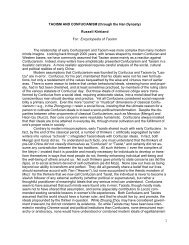
Figure 1 Measles data. Years are grouped together for each county 1985–1991
In addition, log (n ij ) represents an offset corresponding to the natural logarithm of the
number of children in the ith county during the jth year.
Table 1 lists eight models of this general form and the corresponding values of 2times
the maximized loglikelihood ( 2‘) and the Akaike information criterion (AIC). All of
the models in Table 1 except models 2 and 8 were fit with ML. Of these, model 1 is
a (nonmixture) GLMM, model 3 is a mixture model without random effects and
models 4–6 are two component GLMMs with identical fixed effects, but different
assumptions regarding the random effects structure. Among these models, it is clear
that models 1 and 3 fit much worse than the rest, suggesting that a two component
structure and county specific random effects are necessary here. Models 5 and 6 have very
similarvaluesof 2‘, with AIC preferring the more parsimonious model 6. To investigate
whether the mixing probability varied with immunization rate, we refit model 6 with
immunization rate included as a covariate in the linear predictor for logit(p ij ). A
comparison of this model, listed as model 7 in Table 1, with model 6 via either a likelihood
ratio test or a AIC suggests that g 1 ¼ 0. Thus, among the models fit with ML, we prefer
model 6 for these data.
To illustrate the NPML approach, we refit model 6 dropping the assumption of
normality on the random effects. This model is listed as model 8 in Table 1. For model
8, we followed the strategy described by Friedl and Kauermann (2000) and started the
fitting procedure from a large value of m (m ¼ 12), and then reduced m systematically