US Newsprint Demand Forecasts to 2020. International Institute for ...

International Institute for
Applied Systems Analysis
Schlossplatz 1
A-2361 Laxenburg, Austria
Tel: +43 2236 807 342
Fax: +43 2236 71313
E-mail: publications@iiasa.ac.at
Web: www.iiasa.ac.at
Interim Report
IR-01-070
US Newsprint Demand Forecasts to 2020
Lauri Hetemäki (lauri.hetemaki@metla.fi)
Michael Obersteiner (oberstei@iiasa.ac.at) and (oberstei@ihs.ac.at)
Approved by
Sten Nilsson
Leader, Forestry Project
21 December 2001
Interim Reports on work of the International Institute for Applied Systems Analysis receive only
limited review. Views or opinions expressed herein do not necessarily represent those of the
Institute, its National Member Organizations, or other organizations supporting the work.

Contents
1 INTRODUCTION 1
2 BACKGROUND 2
3 EMPIRICAL MODELS 5
3.1 Classical Approach 5
3.2 Bayesian Model 6
3.3 Newspaper Circulation Model 8
4 THE DATA 10
5 EMPIRICAL RESULTS 11
5.1 Time Series Properties 11
5.2 Classical Model 13
5.3 Bayesian Model 18
5.4 Newspaper Circulation Model 19
5.5 Comparing the Forecasts 21
6 SUMMARY AND CONCLUSIONS 22
REFERENCES 24
APPENDIX I: THE BAYESIAN NORMAL-GAMMA REGRESSION MODEL 27
APPENDIX II: TIME SERIES PROPERTIES OF THE DATA 29
APPENDIX III: ESTIMATION RESULTS 37
ii

Abstract
The purpose of this study is to provide projections of newsprint demand for the United
States (US) up to 2020. Three different approaches were used to compute the
projections. First, various specifications of the standard model used in forest product
demand literature, which we call the classical model, were estimated using annual data
from 1971–2000. The results indicated that structural change in the newsprint
consumption pattern took place at the end of the 1980s. The classical model fails to
explain and forecast the structural change. It appears that changes related to the
development of consumers’ preferences and information technology (IT) may have
caused the break down of the widely accepted positive relationship between the gross
domestic product (GDP) and newsprint demand. These observations motivated the
formulation of alternative models. Thus, a Bayesian model that allows industry experts’
prior knowledge about the future demand for newsprint to be included in the projections
was estimated. Also, an ad hoc model, in which newsprint demand is a function of
changes in newspaper circulation, was used to compute projections. Finally, the
forecasts of these models are evaluated along with some of the existing projections.
Besides providing an outlook for US newsprint demand, the study contributes to the
existing literature of long-term forest product demand by raising some methodological
questions and by applying new models to compute projections. Contrary to some recent
projections (e.g., FAO), the results indicate that US newsprint demand is likely to
decline in the long run.
iii

Acknowledgments
The authors are grateful to the Finnish National Technology Agency (Tekes) for
financially supporting this research.
We would like to sincerely thank Peter Ince for providing the information relating to the
RPA projection.
iv

About the Authors
While working on this paper, Lauri Hetemäki was a visiting senior research fellow at
the Fisher Center for the Strategic Use of Information Technology, University of
California, Berkeley, USA. His home institute is the Finnish Forest Research Institute
(METLA), Finland. Michael Obersteiner is a research scholar in IIASA’s Forestry
Project as well as at the Institute for Advanced Studies, Vienna, Austria.
v

US Newsprint Demand Forecasts to 2020
Lauri Hetemäki and Michael Obersteiner
1 Introduction
The subject of newsprint demand has a long tradition in forest products literature.
According to Buongiorno (1996), the first study using econometric methods to analyze
forest product markets was a study by Pringle (1954), in which he analyzed newsprint
demand in the United States (US). Since Pringle’s study, a large number of studies have
been published on this topic. In addition, some organizations, such as the Food and
Agriculture Organization of the United Nations (FAO) and the US Forest Service,
regularly produces (roughly every 5 years) long-term forest products projections, which
also include projections for US newsprint consumption. The purpose of these
projections is, among others, to provide background information for policymaking
concerning the forest sector. The most recent FAO study was published in 1999 and the
US Forest Service study in 2001 (FAO, 1999a; Haynes, 2001).
The US newsprint market is particularly interesting to study due to its global
significance and the methodological challenges it raises. It is the world’s largest
newsprint market, being slightly larger than the whole European market, and consuming
about one third of the world’s total production of newsprint. Roughly about half of this
consumption is based on imported newsprint (mainly from Canada). It is clear that
changes in the US market will also have important implications to world newsprint
markets. Furthermore, the US newsprint market turns out to be a challenging and topical
market to study from the methodological perspective. It appears that since the end of the
1980s, structural change has taken place in newsprint consumption in the US, which the
conventional forest products demand studies fail to explain and forecast. In particular,
the historical relationship between newsprint consumption and economic activity (GDP)
seems to have changed in recent years in the US. Therefore, there is also a need to
reassess the performance of the models used to forecast newsprint demand.
In this study, the long-term US newsprint forecasts are computed using three different
methods. First, various specifications of a model which has dominated forest product
demand literature for decades and which we name the “classical model” are estimated.
In the classical model, the economic activity variable (GDP) and the price of newsprint
are assumed to be the determinants of newsprint demand. Secondly, a Bayesian
variation of the classical model is estimated. This approach allows to include subjective
prior information, such as industry experts’ views, to the estimation and forecasting of
newsprint demand. To our knowledge, Bayesian methods have not yet been applied to
forest economics literature in this way. However, as recent studies show, Bayesian
1

methods can be very useful for forecasting purposes and the approach has become
increasingly popular in applied econometrics (e.g., West and Harrison, 1997; Pole et al.,
1999; Bauwens et al., 1999). The third method used is an ad hoc model, which includes
the changes in newspaper circulation as an explanatory variable, thus named as
“newspaper circulation model”. Although, this model is not derived from economic
theory (like the classical model), it can be justified on the basis of pragmatic reasoning
and prior data analysis.
The results indicate that the sign of elasticity in newsprint demand with respect to GDP
may have turned from positive to negative. Moreover, the GDP parameter is no longer
statistically significant when a post-1987 sample is used for the estimation. Also, the
newsprint price variable does not appear to contain significant explanatory power, if
post-1987 data is used. Finally, the overall conclusion from the various projections is
that the US newsprint demand is likely to decline in the next 20 years.
This paper is organized as follows. Section 2 provides the background for US newsprint
demand projections and discusses some of the existing studies; Section 3 presents the
theoretical and empirical methodology of the different approaches used in the present
study; Section 4 describes the data; Section 5 reports the empirical results; and finally in
Section 6 some conclusions and general remarks are provided.
2 Background
The long-term projections of the future consumption of forest products have significant
practical relevance, since they are likely to influence government policymaking and
private decision-making concerning the forest sector. Indeed, in the US the Forest and
Rangeland Renewable Resources Planning Act of 1974 (RPA) actually requires the
Secretary of Agriculture to periodically conduct assessments of the nation’s renewable
resources and their future development. In order to accomplish this objective, the US
Forest Service produces so-called RPA Timber Assessment studies, which also include
long-term projections for forest product consumption. These types of interests in the US
and other countries sparked significant efforts in the late 1970s to build large scale and
more sophisticated models for forest products projections and forest policy analysis.
The most well known outcomes of these efforts are the TAMM model (Adams and
Haynes, 1980), the GTM model (Kallio et al., 1987), and the PELPS model (Zhang et
al., 1993). 1 These studies, along with the Solberg and Moiseyev (1997) study that
surveys the European forest products modeling literature, give a good picture of the
state-of-the-art in long-term forest products forecasting.
FAO has been publishing long-term projections since the beginning of the 1960s, the
most recent being the FAO (1999a) outlook study. This report, which is based on the
PELPS model, provides projections for global forest products consumption, production,
trade, and prices up to 2010. 2 The most recent RPA Timber Assessment (Haynes, 2001)
1 For a discussion of the projections and the methods see, e.g., Buongiorno (1977; 1996), Baudin and
Brooks (1995), and FAO (1999b).
2 Although FAO (1999a, b) calls its projection model the Global Forest Products Model (GFPM), its
underlying principles are the same as the PELPS model (Zhang et al., 1993).
2

study provides an outlook of the timber situation in the US from 1996 to 2050. Both of
these studies also include long-term projections for US newsprint demand. The FAO
(1999a, b) projections are based on an empirical model, in which the demand for forest
products are determined by economic growth (GDP), real prices of forest products, and
lagged demand. This type of model has been used for decades in forest product demand
literature and could thus be called “a classical model”. Because FAO (1999a) produces
projections for a large number of countries and many product types, for simplicity the
demand equations are estimated for three groups of countries, rather than for each single
country. Thus, the model used to project demand for US newsprint is estimated by using
annual data for 26 high-income countries from 1965 to 1994. The results for the
estimated parameters are shown below:
News. cons. = -0.02 (news. price) + 0.45 (GDP) + 0.46 (lag demand t-1 )
The equation has a good fit; it explains 98% of the historical variations in newsprint
consumption. The long-run price and income elasticities derived from the above
equation are -0.03 and +0.82, respectively. These are in accordance with earlier
elasticity results obtained in the literature (see review in Simangunsong and
Buongiorno, 2001). On the basis of these findings, the FAO model could be regarded as
a reasonable projection model. Moreover, the strength of this model is its the theoretical
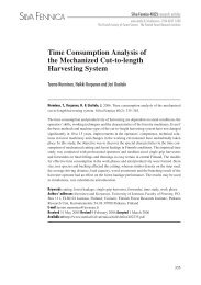
basis and simplicity. From Figure 1, one can observe that the model projects a steadily
increasing demand for newsprint in the US during 1995–2010. In fact, the future trend
follows more or less the historical trend.
mill. tons
16.4
FAO
1995-2010
16
14
12
10.9
I 10.6
RPA 10
2001-2020
8
Year 75 80 85 90 95 00 05 10 15 20
Figure 1: US newsprint consumption projections by FAO (1995–2010) and RPA
(2001–2020).
3

It is also interesting to analyze in more detail the RPA model (Haynes, 2001) ― it is the
most up-to-date model and projection for US newsprint consumption in the literature. It
can be regarded as a classical model, but with some novel features. It was originally
formulated and estimated by Zhang and Buongiorno (1997) using annual data for 1960
to 1991. The RPA demand equation, which is derived from a two-stage Almost Ideal
Demand System (AIDS), and the estimated values of the parameters used for computing
the US newsprint projections (up to 2050) are shown below:
News. cons. = -0.22 (news. price) + 1.23 (GDP pc) + 1.0 (population) – 0.02
(technological change) – 0.95 (print media price) + 0.28 (capital price) –
0.07 (TVs/radios price) – 0.06 (computer price) + 0.1 (demand calibration
dummy).
Besides including the classical explanatory variables (GDP per capita, newsprint price,
population), the model has in addition four price variables and two dummy variables.
Without going into details, the print media price index measures the impact of changes
in the prices of printed materials, which will affect the printing and publishing industry
and thus, in turn, newsprint demand. TV, radio, and computer prices reflect the possible
substitution impacts of electronic media. The price of capital enters the equation due to
the technical structure of the AIDS system. In the RPA equation, the estimated income
and price elasticity parameters have the same signs as the FAO equation, but the
absolute values are greater in the RPA equation.
RPA introduces the demand dummy calibration variable in order to make small
adjustments to demand growth in the historical period of the model (1986–2000) so that
the model is able to track actual historical demand quantities precisely. In addition, the
dummy variable is used to dampen newsprint demand in the first few years of the
projection period (beyond 2000) to reflect the current recession in the US economy and
reduced newsprint demand. Furthermore, in the long run (after 2020), the dummy
reflects assumed gradual substitution of newsprint by electronic media (reducing the
rate of change in newsprint consumption to 70% of that which would otherwise have
been predicted by the econometric formula). In the forecast period, population and GDP
per capita are projected to increase along their historical trends. Relative prices of
capital, printed material, and TVs/radios are assumed to increase modestly in the future
while the price of computers is assumed to decrease over time.
Figure 1 shows that the RPA model projections are very different from FAO. In brief,
the FAO projection reflects the increasing trend of pre-1987 data, whereas the RPA
projection reflects the stagnating post-1987 trend. The difference between the two
projections in 2010 is 5.5 million tons, which is equal to the annual production of
roughly 16 modern newsprint mills (the total US production of newsprint in 2000 was
6.7 million tons). Both from the methodological and practical policy perspectives, it
would be important to try to resolve which of the forecasts, if either, is the more
plausible.
The apparent structural change in the newsprint demand pattern after 1987, indicated by
Figure 1, suggest that one should study in more detail the applicability of the classical
newsprint demand models to compute future long-term forecasts for US newsprint
4

consumption. The classical model implicitly assumes that the structure and behavior of
the forest product markets remains the same as in the past. In particular, the projections
are very sensitive to the assumptions concerning GDP growth. Besides the importance
of being able to accurately forecast the future GDP growth rate, it is important that the
relationship between economic activity and demand for forest products remains stable.
For the US, however, the relationship between newsprint consumption and GDP growth
appears to have changed recently (see Section 5.1).
The RPA model acknowledges the recent structural changes and introduces dummy
variables and the impact of electronic media to try to capture these changes to
projections. The model implies that the relative prices between newsprint and electronic
media are important determinants of newsprint demand. However, the underlying
structure of the model is still the classical type, with GDP and the newsprint price
variable playing an important role. Moreover, the dummy variables do not explain why
the structural changes have taken place.
In summary, the results from the literature and the data indicate that it is necessary to
analyze in more detail the apparent structural change in US newsprint demand, and the
ability of the conventional models to explain the more recent data. Also, there seems to
be a need to experiment with new types of models that would reflect the recent changes
in consumers’ media behavior, and could be used for long-term forecasting purposes.
3 Empirical Models
In this Section, the empirical models used to project newsprint demand in the US from
2001 to 2020 are presented. First, the “classical” model commonly used in forest
economics literature is presented. Then the Bayesian approach is described, and finally
the so-called “newspaper circulation model” is outlined.
3.1 Classical Approach
The basic structure of the econometric models used to project forest products demand
has not changed significantly over time (see, e.g., McKillop, 1967; Kallio et al., 1987;
Solberg and Moiseyev, 1997; Simangunsong and Buongiorno, 2001). Typically, the
theoretical background of the models is production theory, according to which the forest
product enters as an intermediate input in the manufacturing production function along
with other inputs. Assuming a behavioral hypothesis, e.g., cost minimization, allows
one to formulate an optimization problem from which the demand for the forest product
can be derived. Typically, this setting produces a demand function, such as the one in
the Global Forest Products Model (GFPM) (FAO, 1999a, b) and in Simangunsong and
Buongiorno (2001), and expressed as equation (3.1):
D
ik
ik
σik
ik
aσ
ik
ik
η
= a P X D , (3.1)
ik
ik , −1
where Dik
is the demand in the ith country for commodity k, D−
1
is demand in the
previous year, P is the price of the commodity, X is gross domestic product, and σ , α , η
5

are the elasticities with respect to price, GDP, and past demand. For example, in the
present case, i denotes the US and k denotes newsprint. The empirical model
corresponding to equation (3.1), after logarithmic transformation and using the
empirical data corresponding to the theoretical variables, can be written as:
ln( d
1
) news t
= a + β ln( p ) news t
+ β ln( GDP ) USA t
+ β ln( d )
, 0 1
, 2
, 3 news,
t− + ε
t
, (3.2)
where d
news, t
is the quantity of newsprint consumption in the US, p
news, t
is the real price
of newsprint, GDP
USA , t
is the real gross domestic product in the US, dnews, t −1
is a lagged
dependent variable measuring the possibility that in the short-run demand may adjust
only partially, ε
t
is the error term, and t is a subscript denoting the time period. Since
the variables are in logarithmic form, the β -parameters can be interpreted directly as
elasticities. Typically, the studies assume that the signs of the elasticities are known a
priori. For example, Simangunsong and Buongiorno (2001:161) state that on the basis
of the universality of economic laws of demand “one would expect the price elasticity
of demand to be non-positive and the GDP elasticity to be non-negative”. Inorderto
guarantee that the elasticities get correct signs and magnitudes, they can be restricted or
directed in empirical estimation to fulfill this objective. Indeed, in Simangunsong and
Buongiorno (2001) the so-called Stein-rule shrinkage estimator is used for this purpose.
In the present study, various specifications of equation (3.2) are used to estimate the
demand for US newsprint demand and to compute long-term forecasts. However, in the
estimation process, the signs or absolute values of the elasticities are not restricted.
Also, the performance of the model is analyzed by estimating it for different data
samples, and by formally testing whether structural change has taken place.
3.2 Bayesian Model
The motivation for using the Bayesian model is the acknowledgement that besides the
historical time series data, there can be other information that is helpful in making longterm
projections. For example, forest industry experts may have reasonable and useful
views about future forest products market developments. Through their experience and
knowledge about the industry, technology, and markets experts may have information
that can help to project future newsprint consumption patterns. Therefore, by
incorporating subjective expert views, one may be able to improve on the information
set on which the “classical” projections are based. The Bayesian approach provides one
possible method to coherently incorporate this type of information into econometric
forecasting models.
Bayesian methods have become increasingly popular in empirical applications in recent
decade (see, e.g., Bauwens et al., 1999; West and Harrison, 1997). 3 Indeed, current the
literature is so large that one can identify many different methods within the Bayesian
approach. However, to our knowledge, the genuine Bayesian estimation with informed
3 Important factors behind this popularity are the increasing computer capacity and availability of software
packages for Bayesian estimation.
6

priors has not been previously applied in forest products demand literature. 4 A number
of Bayesian textbooks exist that explain the principles and differences of this approach
relative to the frequentist statistical methods (e.g., Pole et al., 1999; West and Harrison,
1997). Here, only a brief description of one particular Bayesian method and the
motivation of using it to forecast long-run newsprint demand in the US are given.
The starting point of our Bayesian framework is the above classical demand model.
However, the Bayesian model allows the industry experts’ knowledge about the
relationship between newsprint consumption and GDP growth to be incorporated in the
estimation. For example, if the industry experts believe that GDP growth does not have
an impact on newsprint demand in the future, one could reset the mean value of the
prior distribution of GDP accordingly. Notationally, this can be expressed as moving
from the classical model or pure model based prior p( GDP t
D t− 1)
to the Bayesian postintervention
prior p( GDPt
Dt− 1,
I
t
) ,where I t
denotes the external information available
from the experts at time t. I
t
is called the prior information set and hereafter prior. The
prior of GDP is then combined with the information from observed data that is
quantified probabilistically by the likelihood function. The resulting synthesis of prior
and likelihood information is the posterior distribution of information. In other words,
the posterior distribution quantifies the collection of the industry experts’ beliefs about
the GDP and the information gained from inference using historical data.
The Bayesian framework in the present study is also based on the classical equation
[equation (3.2)] but, unlike the “frequentist approach”, the Bayesian model assumes a
prior distribution for the GDP parameter ( β
2
). In this case, we used an informed prior
for the estimation of β
2
, while all of the other parameters in equation (3.2) were
derived using a so-called diffuse prior adding no additional information to the parameter
estimation other than historical data.
Obviously, the choice of a particular prior distribution for the GDP parameter can have
substantial impact on posterior model probabilities and the results. The technical details
on how the industry experts’ “informed prior information” is incorporated in our
Bayesian econometric model is described in Appendix I. Here, we only present the
general idea.
The Bayesian parameters (posteriori) were estimated using the Normal-Gamma
regression model. The Normal-Gamma model is a mixed distribution model where prior
information is assumed to be distributed according to a gamma distribution, which is
combined with normally distributed parameters from time-series data. The estimation
method used is ordinary least squares (OLS), as described in equations (A6) and (A7) in
Appendix I. As prior information, we used information that was derived from US
newsprint consumption scenarios that three industry experts produced. Scenarios for
newsprint consumption were established by the industry experts up to 2013 in 5-year
intervals from 1998 onward. The methodology is briefly described in Section 4 and
4 Simangunsong and Buongiorno (2001) use an “iterative empirical Bayesian estimator”, which is
basically a Stein-rule shrinkage estimator in the dynamic setting. The approach is qualitatively different
from the Bayesian method used here.
7

more detail is given in Obersteiner and Nilsson (2000). From the historical time series
data and the information provided by the experts, a panel data set was constructed and
used to estimate equation 3.2. For the parameter estimation of the ‘expert model’ we
used the OLS fixed effects estimator. Finally, for the computation of the Normal-
Gamma regression model, the newsprint consumption data for the period 1987–2000
was used.
3.3 Newspaper Circulation Model
The data on US newsprint consumption, GDP, and newsprint price indicate that the
historical relationship between these variables appears to have changed after 1987 (see
Section 5 and Figure 4 for more details). Therefore, it is of interest to analyze whether
other variables exist that could explain the recent changes in the newsprint market and
contain important “causal” relationship to newsprint demand. Here, we experiment with
a model that uses changes in newspaper circulation as an explanatory variable, which
we therefore name “the newsprint circulation model”.
Unlike the classical model, our newsprint circulation model is not derived from
economic theory, but it is an ad hoc type of model. However, pragmatic reasoning and
statistical analysis of the underlying data suggest that changes in newspaper circulation
may be an important determinant of newsprint consumption. It appears logical to think,
that the more (less) people read newspapers, and thus the higher (lower) the newspaper
circulation is, the more (less) there is also demand for newsprint. In Figure 2 the
newspaper circulation in the US, along with population development, are shown for the
period 1940–2000. The figure shows that after 1980 the volume of daily newspaper
circulation has stagnated and from 1987 onwards has actually started to decline, despite
the continued increase in the population. Thus, in the US people read fewer newspapers
than previously. Furthermore, from Figure 3, which shows the annual changes in
newspaper circulation and the newsprint consumption for 1987–2000, it is evident that
the two series follow a very similar pattern. This is what we would expect since, ceteris
paribus, the smaller the circulation the less demand there is for newsprint. 5 Finally, we
analyzed the “causality relationship” between changes in newspaper circulation and
newsprint consumption using the Granger causality test. Granger causality measures
precedence and information content between two variables, but does not by itself
indicate causality in the more common use of the term. Therefore, the test does not
necessarily imply that newsprint consumption is the effect or the result of newspaper
circulation, although it could be. Bearing this in mind, the test results indicated that
newspaper consumption is “Granger-caused” by newspaper circulation, but not vice
versa. 6
5 From analyzing the simple correlation coefficients and running the Granger causality tests for various
specifications of the newspaper circulation variable, the results indicated that it is indeed the change in
newspaper circulation rather than its level that is more closely related to newsprint consumption.
6 The Granger causality test equation included lagged (one and two periods) newsprint consumption and
the changes of newsprint circulation variable. The newsprint circulation turned out to be a statistically
significant determinant of the newsprint consumption, but not vice versa. Thus, there is no two-way
Granger causality present in these series.
8

Circulation / mill.
Population / mill.
Population
240
60
55
50
45
Circulation
200
160
1940 1950 1960 1970 1980 1990 2000
Figure 2: Newspaper circulation volumes and population in the US, 1940–2000.
normalized data
2
1
Newsprint consumption
0
-1
-2
-3
Circulation change
1988 1990 1992 1994 1996 1998 2000
Figure 3: Newsprint consumption and changes in newspaper circulation in the US,
1987–2000 (data values normalized around zero).
9

On the basis of the above reasoning, the following model to forecast newsprint demand
was formulated in logarithmic form:
ln( d news t ) = γ 0 + γ1∆
ln( circnews,
t ) + γ 2 ln( dnews,
t − 1 ) + µ t
, (3.3)
where ( d
news ,t
) is the quantity of newsprint consumption in the US, ∆( circ news ,t
) is the
change in the volume of newspaper circulation, dnews, t −1
is lagged dependent variable
measuring the short-run dynamics in demand, µ
t
is the error term, and t is a subscript
denoting the time period. We would expect the γ1-parameter to have a positive sign,
since an increase in circulation should cause an increase in newsprint consumption.
4 The Data
The data used to estimate the different models consisted of 30 observations from 1971
to 2000, or its two sub-periods: 1971–1987 and 1987–2000. Because of the tendency for
economic time series to exhibit variations that increase in mean and dispersion in
proportion to the absolute level of the series, we follow the common practice and
transform the data by taking logarithms prior to analysis. This transformation also
allows us to interpret the estimated parameters as elasticities in the demand equations.
The newsprint consumption variable used refers to uncoated paper, unsized (or only
slightly sized), containing at least 60% (percentage of fibrous content) mechanical wood
pulp, usually weighing not less that 40 g/square meter and generally not more than 57
g/square meter of the type mainly used for printing newspapers. Most newsprint is used
to print daily and weekly newspapers. The other major uses are inserts, flyers,
newspaper supplements, and directories. The data for the years 1980–2000 is obtained
from Newspaper Association of America (NAA). For the years 1971–1979, the FAO
data for apparent newsprint consumption was used. Since the FAO figures are on
average 4.9% higher than the figures reported by NAA, the observations for 1971–1979
were scaled down by this percentage. NAA data measures the actual consumption,
whereas FAO data measures the apparent consumption, which includes the inventory.
However, the qualitative results are not sensitive to whether one uses the NAA or FAO
data. [Sources: Newspaper Association of America (primary sources: Canadian Pulp
and Paper Products Council, US Department of Commerce); FAOSTAT online
database.]
Newsprint price is the transaction price of yearly averages for 48.8 gram standard
newsprint (Eastern US prices). The nominal price is transferred to real price by deflating
it using an implicit price deflator for personal consumption expenditures. For the years
2000 to 2020, it is assumed that the price of newsprint stays at its 1999 level. [Sources:
Newspaper Association of America (primary source: Resource Information Systems
Inc; US Bureau of Economic Analysis (http://www.bea.doc.gov).]
The US real gross domestic product (GDP) data (both in per capita and at the country
level) refers to GDP in 1996 prices (US$). The data was obtained from the US Bureau
of Economic Analysis, Department of Commerce. It is assumed that real GDP will grow
10

y 2.40% annually between 2001 and 2020. This is the same assumption that FAO
(1999a) uses for its projections for the US from 1995 to 2010. The population data and
projections for 2020 refer to mid-year population and were obtained from the US
Census Bureau.
The US daily newspaper circulation refers to volume number in millions. [Source:
Newspaper Association of America (http://www.naa.org/info/facts01/index.html).]
For the derivation of the Bayesian prior, the scenario plots constructed by a group of
research and development (R&D) managers of the paper industry were used. The
experts participated in an online course on ‘Managing Technology for Value Delivery’
at the University of British Columbia (Procter, 2000), in which scenarios for future US
newsprint demand were formulated. The expert group used a methodology for scenario
plotting developed by Obersteiner and Nilsson (2000). According to this methodology,
course participants were asked to give quantitative input for about three main force
factors determining the development of the US newsprint market. These force factors
were: (1) economic and life style development, (2) substitution of newspaper content
between paper and electronic media, and (3) newsprint intensity of newspaper making
(basically future changes in the weight and size of the average newspaper). These
factors were allowed to vary for different population cohorts, distinguished by gender,
age, and education, in order to model demographic shifts due to ageing and education
triggered changes in the consumption pattern. Population trajectories were computed by
IIASA’s Population Project (Lutz and Goujon, 2001) and were, thus, exogenous
information to the experts. After the initial scenarios were formulated, they were
iteratively discussed, commented and improved by course participants.
There were only three experts that provided full scenarios during the course. It is clear
that the number of experts is very small, and therefore the results may not be
generalized to reflect the view of the whole industry, but rather represents a case study.
However, from the Bayesian methodological point of view, the small number of experts
is not a critical issue for being able to use the method.
5 Empirical Results
5.1 Time Series Properties
Before the actual estimation of the different models, the time series properties of the
underlying data were analyzed using graphs, autocorrelation functions, Augmented
Dickey-Fuller (ADF) and Philips-Perron (PP) tests, and various cointegration tests. The
results indicated that newsprint consumption, GDP, and newsprint price series are nonstationary
series (the results are shown in Appendix II). 7 The various cointegration test
results pointed to the possibility of either zero or one cointegration relationship between
these variables. The newspaper circulation change series is on the border of being a I(0)
7 The ADF tests were run both with and without the deterministic trend. According to the ADF test results,
newsprint consumption, GDP, and price series can be regarded as I(1)-series at the 5% significance level.
11

or I(1) series ― the null hypothesis of non-stationarity can almost be rejected at the 5%
level. The correlogram and the graph of the series suggest that it is a stationary series.
What implications should the above unit root and cointegration test results have to
modeling, estimation, and interpretation of the results Clearly, when there are nonstationary
variables in the models, particular concern should be attached to the
possibility of spurious regressions and biases in standard errors. However, from the
model strategy perspective, the results do not give unambiguous guidance. For example,
in a recent survey, Allen and Fields (1999) conclude that the econometric literature
gives no generally accepted principles on how one should utilize the unit root and
cointegration test results for model strategy. In the present study, this question is made
even more difficult due to the small sample, which casts doubt as to the robustness of
unit root and cointegration tests, and also makes it difficult to estimate equations with
large number of variables or systems models (in some specifications only 14
observations were used, see below). In the present study, a strategy of trying to keep the
model specifications as simple as possible, given that the specifications were still
statistically robust on basis of a number of different miss-specification tests, was
chosen.
The initial analysis of the graphs and descriptive statistics of the data indicated that it
would be informative to estimate the models for various sample periods. Figure 4 shows
the newsprint consumption, real price, and real GDP series for the period 1971–2000
(the series are in logarithms and normalized around 0). The trend in newsprint
consumption increased during 1971–1987, except for the periods relating to the oil
crises (1973–1975 and 1980–1982). After 1987, newsprint consumption started to
stagnate, indicating a structural change in the pattern. Figure 4 also shows that the
reason for stagnating newsprint consumption is probably not related to GDP or
newsprint price, since real GDP has continued to increase along its long-run trend and
real newsprint price has continued its declining trend. 8 These changing patterns between
the series can also be observed in the simple correlation coefficients shown in Table 1.
For the sample period, 1971–1987, the correlation coefficient between newsprint
consumption and real GDP is positive and very high (0.91), while for the period 1987–
2000 it is negative and markedly lower (-0.25). Similarly, major changes in the signs
and absolute values of the correlation coefficients between newsprint consumption and
price series, and between price series and GDP has taken place. However, when
interpreting the latter correlation coefficients, one should be aware of the significant
jump in the price series during 1995–1996.
In summary, the data analysis shows that the results are likely to be very sensitive to the
particular sample period used for the estimation. This suggests that one should
experiment with estimating the models for various time periods, instead of only using
thewholesampleperioddata.
8 Also, the stagnation cannot be related to population growth, since it has also continued to increase along
the long-run trend.
12

2
1
Normalized values
Newsprint
GDP
0
-1
-2
Price
-3
Year 1975 1980 1985 1990 1995 2000
Figure 4: US newsprint consumption, real GDP, and real newsprint price, 1971–2000.
Table 1: Correlation coefficients.
LNEWS 1971–2000
1971–1987
1987–2000
LGDP 1971–2000
1971–1987
1987–2000
SAMPLE LGDP LPRICER
0.85
0.91
-0.25
-0.48
-0.09
0.29
-0.65
0.27
-0.59
5.2 Classical Model
Due to the structural break in the data, estimations of the classical model were
computed for the following three periods: 1971–2000, 1971–1987, and 1987–2000. The
latter two sub-periods have very few observations (17 and 14, respectively) and the
results should therefore be interpreted with caution. Still, the sub-period estimations are
likely to produce more meaningful results than using the whole sample. Besides
estimating the basic classical model for different observation periods, three different
model specifications were also estimated. Because of possible simultaneity between the
newsprint consumption and its price, a simple vector-autoregressive (VAR) systems
model was also estimated. Moreover, a static version of the classical model was
computed. Finally, a specification where the impact of population changes were
incorporated by using the newsprint consumption per capita as an dependent variable
and the GDP per capita as an explanatory variable was computed. Table 2 provides the
summary of the estimation results.
13

Table 2: Estimation results.
MODEL
estimated
period
Constant
sr
GDP
lr
GDP
sr
Price
lr
Price
Lagged
Demand
∆ Newsp.
Circulat.
_ 2
R
B-G serial
correlation
5% level
1. Classical
1971–2000
2. Classical
VAR
1971–2000
3. Classical
1971–1987
4. Classical
1987–2000
5. Classical
Static
1971–2000
6. Classical
Per Capita
1971–2000
7. Bayesian
Prior Panel
1989–2013
8. Bayesian
Posterior
1987–2000
9. Newspaper
Circulation
1987–2000
-0.09
(0.17)
-0.35
(0.70)
3.07
(5.12)
0.93
(0.80)
-1.61
(2.41)
0.68
(0.71)
1.10
(2.30)
0.92
(0.46)
1.25
(6.43)
0.08
(1.05)
0.09
(1.22)
0.70
(6.57)
-0.01
(0.07)
0.03
(1.20)
-0.06
(2.22)
-0.02
(0.10)
0.33 -0.01
(0.17)
0.09 0.05
(0.80)
0.84 -0.49
(4.79)
-0.01 -0.02
(0.30)
0.44
(7.18)
0.13 -0.01
(0.11)
-0.54
(5.09)
-0.04
(0.24)
-0.05 0.77
(6.09)
0.05 0.79
(6.02)
-0.58 0.16
(1.18)
-0.06 0.66
(2.01)
0.09
(0.91)
-0.01 0.76
(6.15)
1.14
(22.79)
0.71
(1.17)
0.51
(6.47)
3.11
(10.56)
0.87 No
0.87 No
0.95 No
0.17 No
0.72 Yes
0.87 No
0.98 No
No
0.92 No
Note: t-values are in parentheses.
In Table 2, the Models 1 to 6 show the results for various specifications of the classical
frequentist models. For the dynamic specifications (i.e., models with lagged dependent
variable) both the short-run (sr) and long-run (lr) GDP and price elasticities were
computed. Also, the respective t-values are shown in parentheses, the adjusted
_ 2
coefficient of determination ( R ), and the conclusions from the Breusch-Godfrey (B-G)
LM test for second order serial correlation at the 5% significance level are shown (for a
more detailed report of the estimation results, see Appendix III). 9
9 The assumption of OLS requires the error term to be normally distributed (if this does not hold, e.g., the
t- andR 2 -values may be biased). The Doornik-Hansen test results indicated that all the other models
except Model 4 have non-normal residuals. Further analysis indicated that the reason for the nonnormality
is due to two outlier observations related to the oil crises. By including a dummy variable,
which took value 1 in 1975 and 1982 and zero otherwise, resulted in normally distributed error terms in
Models 1–3 and 5–6.
14

In analyzing how well the different specifications succeed in explaining the historical
_ 2
changes in newsprint consumption ( R -statistics, t-values), Model 3 appears to best fit
the data and Model 4 the worst. Thus, the classical model does not seem to be able to
explain the changes in the US newsprint consumption during 1987–2000. This was also
confirmed by a Chow breakpoint test, which tested whether the same classical
newsprint demand model (Model 1) could be used to describe the data before and after
1987. The test results decisively rejected the null hypothesis of no structural change in
the demand function. The structural change can also be observed from Figure 5,
showing the cumulative sum of the recursive residuals (CUSUM) together with the 5%
critical lines. If the equation (i.e., the parameters of the equation) remains constant, the
CUSUM line will wander close to the zero mean value line. In the figure, after 1987 the
CUSUM line starts to sharply diverge from the mean line, and in 1996 onwards falls
below the 5% critical lines. Thus, the recursive residuals clearly indicate instability in
the equation after 1987.
15
10
5%
5
0
-5
-10
5%
CUSUM
-15
1980 1985 1990 1995 2000
Figure 5: The cumulative sum of the recursive residuals (CUSUM) of Model 1.
The long-run elasticity estimates for Model 3 show that during the period 1971–1987
newsprint consumption is rather responsive to the changes in GDP and newsprint price
(0.84 and -0.58, respectively). Indeed, the GDP elasticity is very close to the elasticity
of 0.82 obtained by FAO (1999a) for the group of high-income countries (the price
elasticity in the FAO study was -0.03). However, Table 2 shows that for the
specifications, including the data up to 2000, the estimated GDP elasticity has a
markedly lower absolute value. If the data sample consists only of post-1987
observations, the elasticity obtains a negative sign (Model 4). Figure 6 also illustrates
these changes, where the recursive coefficient estimates for GDP are shown with two
respective standard error bands. The GDP elasticity coefficient displays significant
variation as more data is added to the estimating equation, indicating instability. At the
beginning of the sample the absolute value is above 0.8, but after 1987 there is a sharp
15

decline in the absolute value of the coefficient and it approaches zero when more recent
data is used to estimate the coefficient.
1.2
1.0
0.8
0.6
+2*S.E.
0.4
0.2
GDP elast.
0.0
-2*S.E.
-0.2
80 82 84 86 88 90 92 94 96 98 00
Figure 6: Recursive coefficient estimates for GDP.
The results in Table 2 show that the static specification (Model 5) has a problem with
serial correlation, indicating that some dynamics is necessary. However, the absolute
value of the GDP elasticity is of similar magnitude in the static and dynamic
specifications. The per capita specification (Model 6) produces lower absolute values
for GDP and price elasticities, but they are also statistically insignificant.
The above models were used for forecasting US newsprint demand up to 2020.
Forecasts of the present study are ex post dynamic forecasts from the different
specifications. Dynamic forecasts involve multi-step forecasts starting from the first
period in the forecast sample (1988–2020 or 2001–2020). Unlike in static forecasts, the
previous period error is not checked, nor are corrections for errors incorporated in
subsequent forecasts. 10 Therefore, newsprint forecasts do not benefit from knowing the
newsprint in the previous time period or knowing the previous forecast errors. For the
values of the exogenous variables in the forecast horizon, the following assumptions
were made. The real GDP is assumed to grow at the same rate as assumed in FAO
(1999a), i.e., by 2.40% annually between 2001 and 2020 (the mean figure for 1971–
2000 is 3.30%). For the newsprint price we assume that it stays at its 2000 level for
2001–2020.
10 A static forecast produces a sequence of one-step-ahead forecasts, using actual rather than forecasted
values for the lagged dependent variables.
16

The forecast results for 2010 and 2020 are shown in Table 3. First, the FAO (1999a) and
RPA (Haynes, 2001) projections are shown. 11 FAO’s projection is based on estimating a
classical newsprint demand equation using data up to 1994 and making forecasts from
1995 to 2010. Model 3 is estimated using data from 1971–1987 and forecasts are for the
period 1988–2020. All the other specifications provide forecasts from 2001 to 2020
(RPA actually provides projections up to 2050).
Table 3: Forecasts for US newsprint consumption (in millions metric tons).
MODEL 1994 2000 2010 2020
Actual values 11.9 12.2
FAO (1999a) 13.5 16.4
RPA (Haynes, 2001) 10.9 10.6
1. Classical 1971–2000 13.9 15.1
2. Classical VAR 1971–2000 13.3 14.3
3. Classical 1971–1987 18.0 21.8 26.8 32.7
4. Classical 1987–2000 11.9 11.8
5. Classical Static 1971–2000 14.4 15.9
6. Classical Per Capita 1971–2000 15.3 17.3
7. Bayesian Prior Panel 1989–2013 11.9 11.7
8. Bayesian Posterior 1987–2000 12.1 11.9
9. Newspaper Circulation 1987–2000 11.1 7.4
Model 3 (1971–1987) generates the highest forecasts and Model 4 (1987–2000) the
lowest. Comparing the projections of Model 3 to actual data for 1988–2000, we can
infer that Model 3 overestimates the actual figures in 2000 by roughly 80%. Similarly,
the FAO (1999a) forecast overestimates the 2000 figure by 11%. The evolvement of the
forecasts over time is also shown in Figure 7. It shows that Model 3 projects increasing
consumption during 2000 to 2020, more or less along the pre-1987 historical trend.
Model 1 projects slightly increasing consumption, whereas Model 4 takes the post-
1987 structural change into account, and projects stagnating consumption.
In summary, the estimation results point consistently towards a historically important
structural change in the US newsprint consumption after 1987. None of the different
specifications of the classical model provided statistically satisfactory results for the
data after 1987. Also, one implication of the results is that, for the newsprint demand in
US, the universality of economic laws of demand that are interpreted to require nonnegative
GDP elasticity (cf. Simangunsong and Buongiorno, 2001), may not hold.
Finally, the results clearly point towards a need to develop new models that are more
capable in explaining the recent behavior of newsprint markets in the US.
11 It should be noted that FAO provides three different projections: low, median, and high, depending on
the particular assumptions imposed. The discussion in this study is based on FAO’s (1999a) median
scenario, which is considered to be the “most likely”.
17

Model 3
mill. tons
36
32
28
24
20
Model 1
16
12
Model 4
8
Year00 02 04 06 08 10 12 14 16 18 20
Figure 7: Forecasts from classical models, 2001–2020.
5.3 Bayesian Model
The Bayesian Prior model (Model 7) was estimated using the panel data set that was
constructed from the information provided by the experts and, thus, reflects the
‘consensus’ of the industry experts. For the estimation of the Bayesian Posterior model
(Model 8), we used the second moment of the GDP elasticity of the expert model as an
informed prior. For the newsprint price and lagged demand parameters the so-called
diffuse priors, which are technically equivalent to large second moments, were used.
The use of diffuse priors is due to the fact that experts were not required to make
specific assumptions on prices or lagged demand. 12
The absolute values of the estimated parameters for Models 7 and 8 are very close (see
Table 2). The GDP elasticity of the Bayesian Posteriori model is, at two decimal points,
equal to the GDP elasticity of the expert model (Model 7). This is due to the prior high
precision of the GDP elasticity from the experts. On the other hand, the values of the
estimated parameters for newsprint price and lagged demand differ somewhat between
Model 7 and Model 8. Figure 8 shows that the forecasts produced by Model 7 are only
slightly lower than Model 8 projections. Moreover, the projections indicate a rather
small decline over time in newsprint consumption ― a drop of about 0.3 or 0.4 million
ton in 20 years. Comparing the Bayesian estimation results to the classical model using
the same sample observations (Model 4), it is interesting to note the similarity of the
estimates and forecasts. Thus, in this study the use of expert information does not
12 Due to this assumption the information contained in the second moments were not directly used as
priors for H * . Furthermore, official newsprint prices reflect only spot market fluctuations and exclude the
large volumes traded on long-term contracts and are, thus, not fully informative.
18

change the projections due to the fact that the experts’ views in the present case seem to
reflect the implications of recent historical data. However, the projections would
diverge if the experts’ views would be different to the projections that are consistent
with historical data.
In the present study, the Bayesian framework was used to set a prior distribution only
for the GDP parameter. The natural extension of this approach would be to set a prior
also for the newsprint price parameter. Furthermore, a key aspect of the model is the
uncertainty related to the choice of the regressors, i.e., model uncertainty. Thus, we
could also specify a prior distribution over the model space (Fernandez et al., 2001).
More importantly, due to the low explanatory power of the GDP and the price
parameter in the US newsprint demand model, one should try to look for new variables
also in the Bayesian setting that could better explain the recent newsprint consumption
behavior.
mill. tons
12.2
12.1
12.0
Model 8
11.9
11.8
Year
Model 7
11.7
00 02 04 06 08 10 12 14 16 18 20
Figure 8: Forecasts from Bayesian models, 2001–2020.
5.4 Newspaper Circulation Model
The newspaper circulation model [equation (3.3)] was estimated using data for the
period 1987–2000. The small sample restricted the number of variables that could be
included in the model. Thus, besides the constant term and the newspaper circulation
variable, only the lagged newsprint demand variable was included. The lagged
dependent variable allowed some dynamics and increased the explanatory power of the
model. The estimated parameters did not appear to suffer from multi-collinearity, since
their absolute values changed only marginally depending on whether the estimated
equation included only one of the explanatory variables or both.
The estimation results of equation 3.3 showed that the specification is acceptable using
the conventional statistical criteria for autocorrelation, residual normality, stationary,
heteroskedasticity, functional form misspecification, and explanatory power (detailed
19

esults shown in Appendix III). However, it should be borne in mind that the robustness
of these results are subject to the problems related to the small sample. The absolute
value of the changes in newspaper circulation parameter indicates that, ceteris paribus,
a 1% increase in newspaper circulation would lead to a 3.1% increase in newsprint
demand (see Table 2). Thus, newsprint demand appears to be very elastic with respect
to circulation.
In order to be able to compute the conditional forecasts, assumptions about the
development of newspaper circulation during 2001 to 2020 had to be made. These were
based on recent data on newspaper circulation and households “consumption” of media,
and on the findings of some recent US media studies (e.g., NAA, 2001; UCLA, 2001).
Looking at historical development from 1987 onwards, when newspaper circulation
started to decline, we observe that circulation declined on average by 0.48% annually
during 1987–2000. However, the annual average rate of decline has accelerated
somewhat, being 0.59% for the last five years. The declining interest in newspapers is
apparent also in the data on media consumption of US households. Table 920 in the
Statistical Abstracts of the United States (2000), shows how many hours households
annually spend on different media. According to these statistics, households spent 10%
less time reading newspapers in 2000 than in 1992, while at the same time increasing
Internet consumption by 2050%. Although the relative change in Internet consumption
is huge, its absolute significance is small due to the very low starting level.
Nevertheless, the underlying tendency is declining newspaper consumption and
simultaneous increase in Internet consumption. A similar pattern was found in a recent
study by the North American Newspaper Association (NAA, 2001:4), which surveyed
the media behavior of a nationally representative sample of 4003 adults, aged 18 and
over. According to the study “The first and perhaps most significant finding of the study
is the decline in penetration of traditional media including newspapers, TV, and radio
and the concurrent rise in the use of the Internet as a source of news and information”.
The study also reports evidence that the two phenomena are connected, i.e., the
increasing usage of the Internet accelerates the decline in newspaper readership. These
findings are supported by other studies, such as the NAA (2001) and UCLA (2001)
survey studies. 13
In the newspaper circulation model, the above data and surveys were interpreted to
imply an increasing rate of decline in newspaper circulation in the US during 2001 to
2020. In particular, we assumed that US newspaper circulation is declining by 1%
annually during 2001–2005, by 2% annually during 2006–2010, by 4% annually during
2011–2015, and by 8% annually during 2016–2020. These numbers are ad hoc, and
should not be taken as precise projections, but rather as one possible scenario for
newspaper circulation development. More important than the absolute numbers is the
general trend. The above numbers assume that no dramatic change is taking place and
that the rate of circulation decline increases steadily. We regard the assumptions to be
moderate rather than extreme.
13 It may be noted, that newsprint consumption is stagnating also in Japan and in some European
countries.
20

The dynamic forecasts of the newspaper circulation model based on the above
assumptions are shown in Figure 9. According to the projection, newsprint consumption
is declining rather steadily up to 2010, after which the speed of decline increases. This
pattern clearly reflects the assumptions made about the newspaper circulation decline.
The newsprint circulation model forecast that in 2020 the newsprint consumption would
be 7.6 million tons, which is equivalent to the level last experienced in the mid-1960s.
mill. tons
13
12
11
10
Model 9
9
8
7.6
7
Year 00 02 04 06 08 10 12 14 16 18 20
Figure 9: Forecasts from newspaper circulation model, 2001–2020.
5.5 Comparing the Forecasts
At least the following general conclusions can be drawn from comparing the various
forecasts for US newsprint consumption (see Figure 10 and Tables 2 and 3). First, the
older the data set used to estimate the forecasting model, the higher the long-term
forecasts will be for US newsprint consumption. Thus, Model 3 (uses data for 1971–
1987) and the FAO model (uses data for 1965–1994) clearly provide the highest
projections. On the other hand, the more up-to-date the data set used to estimate the
model, the worse will be the explanatory power and statistical robustness of the
classical model. Indeed, the sign of the income (GDP) elasticity changes from positive
to negative and becomes statistically insignificant when post-1987 data is used.
Similarly, the newsprint price variable becomes insignificant.
The projections from the RPA model (Haynes, 2001), Model 4, and the Bayesian
models (Models 7 and 8) provide very similar projections. These projections indicate a
slight decline in newsprint consumption from today’s level when moving towards 2020.
Also, the newspaper circulation model (Model 9) provides rather similar forecasts with
these models up to 2010. However, for the period 2010 to 2020, Model 9 provides much
more rapidly declining consumption. If the substitution of electronic media (particularly
the Internet) for newspaper reading accelerates from the rate observed in the last five
21

years or so, the projections of Model 9 may very well turn out to be the most accurate of
the various projections presented in this study.
mill. tons
FAO
16.4
16
14
Model 4
Model 8
RPA
12
10
Year
Model 9 8
7.4
75 80 85 90 95 00 05 10 15 20
Figure 10: Forecasts from various models.
From the practical policy perspective, the differences in the projections are significant
and troubling. Depending on whether newsprint consumption will follow the FAO
projection or instead that of Model 9 or even the RPA projection, very different
adjustments would be required in the US newsprint production and its imports (mainly
from Canada). The FAO projection would imply more or less the “business-as-usual”
pattern for the newsprint industry, while the Model 9 projection would imply major cuts
in domestic productions and imports.
6 Summary and Conclusions
In the present study, forecasts for the US newsprint demand for 2001 to 2020 were
computed using various approaches. The results shed light both on the methodological
questions relating to modeling newsprint demand, as well as providing new forecasts for
newsprint consumption.
The results indicated that the classical forest products demand model, still commonly
used in forest economics literature, could not explain or forecast the recent structural
change in the US newsprint consumption. Both the income (GDP) and newsprint price
variable turned out to be insignificant determinants of newsprint demand. Moreover, the
results of this study indicate that one should not rule out the possibility of negative
22

income elasticity. However, the negative sign of the income elasticity is usually
interpreted in the literature to be inconsistent with the demand theory and reflect an
error in the model, estimation, or data (Simangunsong and Buongiorno, 2001;
Buongiorno et al., 2001). So far, this may not have been a particularly large issue, since
in the literature negative income elasticities for forest products demand are rarely
reported. For example, Simangunsong and Buongiorno (2001) summarize the results
from 9 studies published between 1978 and 2000, and the results show that for the 10
different forest product categories covered (including newsprint), not a single negative
income elasticity was obtained.
Recent data and studies on the US media behavior point out that people read less
newspapers, while simultaneously increasing the consumption of electronic media,
especially the Internet (NAA, 2001; UCLA, 2001). It may be that economic wealth (i.e.,
GDP) is one of the factors that allow this substitution to take place. The higher the GDP,
the more wealth households have to buy relative expensive computers and the services
required, such as Internet accounts and modems. Also, the more households there are
with access to the Internet, the more likely that there is substitution between printed
newspapers and consumption of the Internet. Thus, this could imply negative income
elasticity of demand for newsprint. On the other hand, it may be the case that at some
income level newsprint consumption starts to be independent of income. Our estimation
results suggest that the latter conclusion may be relevant for the US today.
In order to resolve the problems relating to the classical newsprint demand model, we
proposed two alternative approaches ― the Bayesian model and the newspaper
circulation model. The Bayesian model allowed combining historical data with
“forward looking” information concerning the GDP elasticity. This model should,
however, be regarded more as an illustrative case of the Bayesian approach in a familiar
classical setting, rather than a genuine alternative to the classical model. This means it
presented a methodology that allows forest sector analysts to incorporate the ‘future’
into the conventional classical demand model by using informed prior. In future studies,
the Bayesian approach could be extended in a number of ways that would differentiate it
more clearly from the classical framework.
The newspaper circulation model is clearly an alternative to the classical model, since
neither the GDP nor the newsprint price variable are included in forecasting long-term
newsprint consumption. On the basis of pragmatic reasoning and data analysis, it was
concluded that the changes in newspaper circulations could be an important indicator of
future newsprint consumption. Consequently, an ad hoc newspaper circulation model
was formulated and estimated. This very simple model performed rather well. However,
a challenge remains in the future to extend the model to also include variables that could
account for the changes in the size and grammage of newspapers. The latter factors will
also directly affect the demand for newsprint. For example, the size of the average
printed version of a newspaper and the grammage of newsprint is likely to decrease
during 2001 to 2020. The major driving force behind this is the movement of
advertisements (specially classified) to other media, and changes in editorial and other
content to online-newspapers. Thus, these factors will most likely enhance the declining
trend of newsprint demand.
23

The general conclusion from the study is that US newsprint consumption is more likely
to decline than increase in the long-term. Of the various model specifications, the
newsprint circulation model provided the lowest forecasts ― 7.6 million tons for 2020
― which is equivalent of the level last experienced in the mid-1960s.
REFERENCES
Adams, D. and R. Haynes (1980). The 1980 Softwood Timber Assessment Market
Model: Structure, Projections, and Policy Simulation. Forest Science Monograph,
22.
Allen, G. and R. Fields (1999). Econometric Forecasting Principles and Doubts: Unit
Root Testing First, Last, or Never Presented at the 19th International Symposium
on Forecasting, 27–30 June 1999, Washington, DC, USA.
Baudin, A. and D. Brooks (1995). Projections of Forest Products Demand, Supply and
Trade in ETTS V. ECE/TIM/DP/6. United Nations Economic Commission for
Europe, Geneva, Switzerland.
Bauwens, L., M. Lubrano and J.-F. Richard (1999). Bayesian Inference in Dynamic
Econometric Models. Oxford University Press, UK.
Buongiorno, J. (1977). Long-Term Forecasting of Major Forest Products Consumption
in Developed and Developing Economies. Forest Science, Vol. 23, No. 1, pp. 13–
25.
Buongiorno, J. (1996). Forest Sector Modeling: A Synthesis of Econometrics,
Mathematical Programming, and System Dynamics Methods. International
Journal of Forecasting, Vol. 12, pp. 329–343.
Buongiorno, J., C.-S. Liu and J. Turner (2001). Estimating International Wood and
Fiber Utilization Accounts in the Presence of Measurement Errors. Journal of
Forest Economics, 7:2, pp. 101–128.
FAO (1999a). Global Forest Products Consumption, Production, Trade and Prices:
Global Forest Products Model Projections to 2010. Working Paper
GFPOS/WP/01, Food and Agriculture Organization of the United Nations (FAO),
Rome, Italy.
FAO (1999b). The Global Forest Products Model (GFPM): Users Manual and Guide to
Installation. Working Paper GFPOS/WP/02, Food and Agriculture Organization
of the United Nations (FAO), Rome, Italy.
Fernandez, C., E. Ley and M. Steel (2001). Model Uncertainty in Cross-country Growth
Regressions. Journal of Applied Econometrics, Vol. 16, Issue 5, pp. 563–576.
Hamilton, J.D. (1994). Time Series Analysis. Princeton University Press, Princeton,
USA.
Haynes, R. (2001). An Analysis of the Timber Situation in the United States:
1997-2050. General Technical Report PNW-GTR-xxx. USDA Forest Service,
Pacific Northwest Research Station, Portland, Oregon, USA, forthcoming.
24

Hendry, D.F. and J.A. Doornik (1997). Empirical Econometric Modelling using PcGive
9.0 for Windows. International Thomson Business Press, London, UK.
Kallio, M., D.P. Dykstra and C. Binkley, eds. (1987). The Global Forest Sector: An
Analytical Perspective. Wiley, New York, USA.
Lutz, W. and A. Goujon (2001). The World’s Changing Human Capital Stock: Multi-
State Population Projection by Educational Attainment. Population and
Development Review, 27(2), pp. 323–339, June.
McKillop, W.L.M. (1967). Supply and Demand for Forest Products ― An Econometric
Study. Hilgardia, 38 (1), pp. 1–132.
NAA (2001). Leveraging Newspaper Assets: A Study of Changing American Media
Usage Habits, 2000. Research Report. Downloaded from and available on the
Internet: http://www.naa.org. October 2001.
Obersteiner, M. (1998). The Pan Siberian Forest Industry Model (PSFIM): A
Theoretical Concept for Forest Industry Analysis. Interim Report IR-98-033.
International Institute for Applied Systems Analysis, Laxenburg, Austria.
Obersteiner, M. and S. Nilsson (2000). Press-imistic Futures ― Science Based
Concepts and Models to Assess the Long-term Competitiveness of Paper Products
in the Information Age. Interim Report IR-00-059. International Institute for
Applied Systems Analysis, Laxenburg, Austria.
Pole, A., M. West and J. Harrison (1999). Applied Bayesian Forecasting and Time
Series Analysis. Chapman and Hall, USA.
Pringle, S. (1954). An Econometric Analysis of the Demand for Newsprint in the United
States. Ph.D. Dissertation, Syracuse University, USA.
Procter, A. (2000). Managing Technology for Value Delivery. Course Manuscript,
Department of Wood Science, University of British Columbia, Vancouver,
Canada.
Simangunsong, B.C.H. and J. Buongiorno (2001). International Demand Equations for
Forest Products: A Comparison of Methods. Scandinavian Journal of Forest
Research, 16, pp. 155–172.
Solberg, B. and A. Moiseyev, eds. (1997). Demand and Supply Analyses of
Roundwood and Forest Products Markets in Europe ― Overview of Present
Studies. First Workshop of the Concerted Action Project AIR3-CT942288,
Helsinki, Finland, 3–5 November 1995, Helsinki, 1997. EFI Proceedings No. 17,
European Forest Institute (EFI), Helsinki, Finland, 418 p.
Statistical Abstracts of the United States (2000). US Census Bureau. Downloaded from
and available on the Internet: http://www.census.gov/statab/www/.
UCLA (2001). Surveying the Digital Future: Year Two. University of California, Los
Angeles (UCLA) Internet Report 2001, Center for Communication Policy.
Downloaded from and available on the Internet: http://ccp.ucla.edu, 29 November
2001.
West, M. and J. Harrison (1997). Bayesian Forecasting and Dynamic Models.
Springer-Verlag Series in Statistics, USA.
25

Zhang, Y. and J. Buongiorno (1997). Communication Media and Demand for Printing
and Publishing Papers in the United States. Forest Science, Vol. 43, No. 3, pp.
362–377.
Zhang, Y., J. Buongiorno and P. Ince (1993). PELPS III: A Microcomputer Priceendogenous
Linear Programming System for Economic Modeling. Research
Paper FPL-RP-526. USDA Forest Service, Forest Product Laboratory, Madison,
Wisconsin, USA.
26

Appendix I: The Bayesian Normal-Gamma Regression Model
Consider the linear regression model:
Y
t
= x′
t
β + ut
2
where
u t
≈ i.
i.
d.
N(0,
σ )
,
xt
is a (kx1) vector of exogenous explanatory variables,
and β is a (k x1) vector of coefficients. Let
⎡ y1
⎤ ⎡ x1
⎤
⎢
y
⎥ ⎢ ⎥
2
x2
y = ⎢ ⎥ X = ⎢ ⎥
⎢ M ⎥ ⎢ M ⎥
⎢ ⎥ ⎢ ⎥
⎣yT ⎦ ⎣x T ⎦
2
σ and
β are both regarded as
where y is a (T x1)vectorandXisa(Txk)matrix.
2
random variables. The prior distribution for σ is given by the gamma distribution.
2
Instead of describing the prior distribution in terms of the variance σ it is convenient
−2
to take the reciprocal of the variance, σ , which is known as the precision:
−
f ( σ
2
X ) =
∗
∗ N / 2
∗
−2
( )
[( N / 2)
−1
/ 2
] ∗ −2
λ σ exp[ − λ σ / 2]
∗
Γ( N / 2)
∗
where N and
distribution of β conditional on the value for
(A1)
∗
λ are parameters that describe the analyst’s prior information. The prior
2
σ
is given by:
⎧
−2
1
∗
−1/
2 ⎛ 1 ⎞ ′
f ( β σ , X )
H exp⎨⎜
− ⎟
β
2 k / 2
2
(2πσ
)
⎩⎝
(2σ
) ⎠
∗ ∗−1
( β − b ) H ( − b )
=
∗
⎫
⎬
⎭
(A2)
Thus, prior to observation of the sample, the analyst’s best guess for the value of β is
represented by the (k x1) vector b* and the confidence in this guess is summarized by
the (k x k) matrix H*; less confidence is represented by larger diagonal elements of H*.
−
f ( β , σ
2
X )
Thus,
, the joint prior density for β 2
and σ , is given by the product of
−2
f ( β , σ y,
X )
equations (A1) and (A2). The posterior distribution
is described by
the following proposition (see Hamilton, 1994:356–357).
Proposition: 14 −
f ( β , σ
2
X )
Let the prior density
be given by the product of equations
(A1) and (A2), and let the sample likelihood be:
14 For proof see Hamilton (1994:367–369).
27

−2
1 ⎧⎡
1 ⎤
f ( y β , σ , X ) = exp
T / 2 ⎨⎢
2 ⎥
⎩⎣2σ
⎦
2
( 2πσ
)
′
( y − Xβ
) ( y − Xβ
) ⎬ ⎫
⎭
. (A3)
Then the following hold: The joint posterior density of β and
−2
σ
is given by:
−
f ( β , σ
2
−2
−
b,
X ) = f ( β σ , y,
X ) ⋅ f ( σ
2
y,
X )
where the posterior distribution of β is conditional on
−2
∗∗ ∗∗
σ is
( b bH )
N , :
(A4)
⎧
−2
1
∗
−1/
2 ⎛ 1 ⎞ ′
f ( β σ , y,
X )
H exp⎨⎜
− ⎟
β
2 k / 2
2
(2πσ
)
⎩⎝
(2σ
) ⎠
∗∗ ∗∗−1
∗
( β − b ) H ( − b )
=
∗
⎫
⎬
⎭(A5)
with
∗−1
−1
∗− ∗
( H + X ′ X ) ( H b + X y)
∗∗
1
b =
′
(A8)
∗−1 −
( H + X ) 1
H = X . (A7)
∗ ∗
′
Furthermore, the marginal posterior distribution of
∗∗ ∗∗
is Γ( , λ )
−
f ( σ
N :
y,
X ) =
∗∗
∗∗ N / 2
∗∗
−2
( )
( N / 2)
λ / 2 σ
∗∗
Γ( N / 2)
−2
σ
[ −1]
∗∗
exp − λ σ
2
[ / 2]
2 −
, (A8)
with
N ∗
= N
∗
+ T
∗∗
λ
∗ ∗ ′
∗ ′ ∗−1
∗−1
−1
∗
= λ + ( y − Xb) ( y − Xb) + ( b − b ) H ( X ′ X + H ) ( b − b )
(A9)
b ′ ′
−1
for
= ( X X ) X y
the OLS estimator.
The Bayesian estimate of the precision is then given by:
−2
** **
( σ y, X ) N / λ
E =
For a more detailed description of the Normal-Gamma regression model see, e.g.,
Hamilton (1994) and Obersteiner (1998).
28

Appendix II: Time Series Properties of the Data
Descriptive Statistics 1971–2000 (30 observations).
LNEWS LGDP LPRICE
Mean 2.371493 8.662462 1.878485
Median 2.433656 8.668003 1.918916
Maximum 2.515678 9.139757 2.069261
Minimum 2.090307 8.215466 1.569125
Std. Dev. 0.125774 0.266045 0.163494
Skewness -0.611043 0.059246 -0.692173
Kurtosis 2.071733 1.876962 2.222391
Jarque-Bera 2.943965 1.594070 3.151364
Probability 0.229470 0.450663 0.206866
Sum 71.14480 259.8739 56.35454
Sum Sq. Dev. 0.458757 2.052620 0.775182
Descriptive Statistics 1987–2000 (14 observations).
LNEWS LGDP LPRICE LCIRC
Mean 2.471737 8.904916 1.766505 -0.008136
Median 2.473999 8.882356 1.762628 -0.005502
Maximum 2.515678 9.139757 2.036388 0.005170
Minimum 2.407035 8.718222 1.569125 -0.026681
Std. Dev. 0.034614 0.129704 0.162834 0.008616
Skewness -0.262347 0.385616 0.172895 -0.814036
Kurtosis 1.907954 1.996258 1.641699 2.948075
Jarque-Bera 0.856256 0.934673 1.145990 1.547765
Probability 0.651728 0.626669 0.563834 0.461219
Sum 34.60432 124.6688 24.73108 -0.113909
Sum Sq. Dev. 0.015576 0.218702 0.344694 0.000965
Correlation matrix 1971–2000.
LNEWS LGDP LPRICE
LNEWS 1.000000 0.853145 -0.482061
LGDP 0.853145 1.000000 -0.645744
LPRICER -0.482061 -0.645744 1.000000
29

Correlation matrix 1971–1987.
LNEWS LGDP LPRICE
LNEWS 1.000000 0.914902 -0.086354
LGDP 0.914902 1.000000 0.273656
LPRICER -0.086354 0.273656 1.000000
Correlation matrix 1987–2000.
LNEWS LGDP LPRICE LCIRC
LNEWS 1.000000 -0.245365 0.295374 0.836755
LGDP -0.245365 1.000000 -0.555644 -0.115412
LPRICER 0.295374 -0.555644 1.000000 0.071325
LCIRCCH 0.836755 -0.115412 0.071325 1.000000
Correlograms for LNEWS and First Difference of LNEWS: Samples 1971–2000
and 1987–2000.
LNEWS/Sample: 1971–2000/Observations: 30
Autocorrelation Partial Correlation AC PAC Q-Stat Prob
. |*******| . |*******| 1 0.875 0.875 25.319 0.000
. |****** | . | . | 2 0.767 0.011 45.511 0.000
. |***** | . | . | 3 0.681 0.032 61.994 0.000
. |***** | . | . | 4 0.610 0.024 75.713 0.000
. |**** | .**| . | 5 0.471 -0.318 84.214 0.000
. |*** | . | . | 6 0.351 -0.031 89.146 0.000
. |**. | .**| . | 7 0.211 -0.220 91.005 0.000
. |* . | . | . | 8 0.103 -0.002 91.472 0.000
. | . | . | . | 9 -0.006 -0.036 91.474 0.000
. *| . | . |* . | 10 -0.069 0.094 91.706 0.000
First Difference LNEWS/Sample: 1971–2000/Observations: 29
Autocorrelation Partial Correlation AC PAC Q-Stat Prob
. | . | . | . | 1 -0.041 -0.041 0.0537 0.817
. | . | . | . | 2 -0.029 -0.031 0.0815 0.960
.**| . | .**| . | 3 -0.210 -0.213 1.6092 0.657
. |* . | . | . | 4 0.077 0.060 1.8237 0.768
. | . | . | . | 5 0.000 -0.009 1.8237 0.873
. | . | . | . | 6 0.042 0.002 1.8935 0.929
. | . | . | . | 7 0.021 0.054 1.9112 0.965
. | . | . | . | 8 -0.022 -0.026 1.9318 0.983
.**| . | .**| . | 9 -0.198 -0.197 3.6904 0.931
. | . | . | . | 10 -0.039 -0.047 3.7636 0.957
30

LNEWS/Sample: 1987–2000/Observations: 14
Autocorrelation Partial Correlation AC PAC Q-Stat Prob
. |**** | . |**** | 1 0.557 0.557 5.3401 0.021
. |* . | . **| . | 2 0.136 -0.252 5.6841 0.058
. *| . | . *| . | 3 -0.126 -0.124 6.0079 0.111
. *| . | . | . | 4 -0.141 0.054 6.4539 0.168
. | . | . |* . | 5 0.004 0.111 6.4543 0.264
. *| . | .***| . | 6 -0.178 -0.444 7.3456 0.290
.***| . | . *| . | 7 -0.334 -0.105 10.907 0.143
.***| . | . *| . | 8 -0.419 -0.142 17.470 0.026
. **| . | . | . | 9 -0.297 -0.041 21.416 0.011
. | . | . |* . | 10 0.009 0.078 21.421 0.018
First Difference LNEWS/Sample: 1987–2000/Observations: 14
Autocorrelation Partial Correlation AC PAC Q-Stat Prob
. | . | . | . | 1 -0.002 -0.002 9.E-05 0.992
. *| . | . *| . | 2 -0.155 -0.155 0.4474 0.800
. **| . | . **| . | 3 -0.246 -0.253 1.6770 0.642
. *| . | . *| . | 4 -0.065 -0.109 1.7703 0.778
. |***. | . |** . | 5 0.334 0.273 4.5407 0.474
. *| . | . **| . | 6 -0.129 -0.225 5.0087 0.543
. | . | . | . | 7 -0.053 -0.016 5.0970 0.648
. **| . | . *| . | 8 -0.226 -0.166 7.0094 0.536
. *| . | . **| . | 9 -0.167 -0.262 8.2529 0.509
. |* . | . *| . | 10 0.084 -0.141 8.6455 0.566
Correlograms for LGDP and First Difference of LGDP: Samples 1971–2000 and
1987–2000.
LGDP/Sample: 1971–2000/Observations: 30
Autocorrelation Partial Correlation AC PAC Q-Stat Prob
. |*******| . |*******| 1 0.886 0.886 25.959 0.000
. |****** | . | . | 2 0.779 -0.022 46.789 0.000
. |***** | . | . | 3 0.684 -0.007 63.445 0.000
. |**** | . *| . | 4 0.588 -0.062 76.190 0.000
. |**** | . *| . | 5 0.489 -0.065 85.384 0.000
. |*** | . | . | 6 0.399 -0.028 91.767 0.000
. |**. | . | . | 7 0.315 -0.038 95.907 0.000
. |**. | . | . | 8 0.242 -0.007 98.462 0.000
. |* . | . | . | 9 0.172 -0.041 99.817 0.000
. |* . | . *| . | 10 0.100 -0.066 100.30 0.000
31

First Difference LGDP/Sample: 1971–2000/Observations: 29
Autocorrelation Partial Correlation AC PAC Q-Stat Prob
. |* . | . |* . | 1 0.189 0.189 1.1455 0.284
.**| . | .**| . | 2 -0.238 -0.284 3.0351 0.219
.**| . | . *| . | 3 -0.252 -0.159 5.2350 0.155
.**| . | .**| . | 4 -0.241 -0.254 7.3266 0.120
. |* . | . |* . | 5 0.074 0.070 7.5331 0.184
. | . | .**| . | 6 0.013 -0.213 7.5396 0.274
. | . | . *| . | 7 -0.027 -0.060 7.5702 0.372
. |* . | . | . | 8 0.088 0.015 7.9048 0.443
. *| . | .**| . | 9 -0.147 -0.250 8.8701 0.449
. *| . | . *| . | 10 -0.099 -0.101 9.3318 0.501
LGDP/Sample: 1987–2000/Observations: 14
Autocorrelation Partial Correlation AC PAC Q-Stat Prob
. |****** | . |****** | 1 0.758 0.758 9.8876 0.002
. |**** | . *| . | 2 0.544 -0.070 15.411 0.000
. |***. | . *| . | 3 0.355 -0.077 17.980 0.000
. |* . | . *| . | 4 0.185 -0.091 18.747 0.001
. | . | . *| . | 5 0.015 -0.141 18.752 0.002
. *| . | . *| . | 6 -0.130 -0.103 19.222 0.004
. **| . | . *| . | 7 -0.256 -0.127 21.319 0.003
.***| . | . | . | 8 -0.331 -0.054 25.404 0.001
.***| . | . *| . | 9 -0.378 -0.082 31.789 0.000
.***| . | . | . | 10 -0.379 -0.033 39.840 0.000
First Difference LGDP/Sample: 1987–2000/Observations: 14
Autocorrelation Partial Correlation AC PAC Q-Stat Prob
. |***. | . |***. | 1 0.390 0.390 2.6152 0.106
. |* . | . | . | 2 0.140 -0.014 2.9827 0.225
. *| . | . **| . | 3 -0.120 -0.201 3.2759 0.351
. | . | . |* . | 4 0.017 0.163 3.2820 0.512
. *| . | . *| . | 5 -0.072 -0.125 3.4108 0.637
. *| . | . *| . | 6 -0.154 -0.174 4.0785 0.666
. **| . | . *| . | 7 -0.296 -0.160 6.8871 0.441
. **| . | . | . | 8 -0.204 -0.039 8.4438 0.391
. **| . | . **| . | 9 -0.260 -0.233 11.481 0.244
. | . | . |* . | 10 -0.054 0.081 11.647 0.309
32

Correlograms for LPRICE and First Difference of LPRICE: Samples 1971–2000
and 1987–2000.
LPRICE/Sample: 1971–2000/Observations: 30
Autocorrelation Partial Correlation AC PAC Q-Stat Prob
. |****** | . |****** | 1 0.782 0.782 20.248 0.000
. |**** | . *| . | 2 0.554 -0.148 30.773 0.000
. |*** | . | . | 3 0.404 0.058 36.567 0.000
. |**. | . | . | 4 0.279 -0.056 39.445 0.000
. |**. | . |*** | 5 0.317 0.349 43.302 0.000
. |*** | . *| . | 6 0.345 -0.060 48.064 0.000
. |**. | . *| . | 7 0.294 -0.069 51.664 0.000
. |* . | ***| . | 8 0.139 - 0.330 52.502 0.000
. | . | . | . | 9 -0.046 -0.056 52.600 0.000
. *| . | . | . | 10 -0.144 -0.004 53.592 0.000
First Difference LPRICE/Sample: 1971–2000/Observations: 29
Autocorrelation Partial Correlation AC PAC Q-Stat Prob
. | . | . | . | 1 -0.026 -0.026 0.0213 0.884
. *| . | . *| . | 2 -0.094 -0.095 0.3164 0.854
. *| . | . *| . | 3 -0.113 -0.119 0.7559 0.860
.**| . | ***| . | 4 -0.301 -0.326 4.0214 0.403
. |* . | . | . | 5 0.067 0.010 4.1914 0.522
. | . | . *| . | 6 -0.054 -0.152 4.3046 0.636
. |**. | . |**. | 7 0.264 0.215 7.1506 0.413
. |* . | . | . | 8 0.067 -0.030 7.3421 0.500
. *| . | . | . | 9 -0.070 0.014 7.5624 0.579
. | . | . | . | 10 0.008 -0.004 7.5652 0.671
LPRICE/Sample: 1987–2000/Observations: 14
Autocorrelation Partial Correlation AC PAC Q-Stat Prob
. |**** | . |**** | 1 0.569 0.569 5.5799 0.018
. |* . | . **| . | 2 0.121 -0.300 5.8544 0.054
. *| . | . *| . | 3 -0.178 -0.157 6.4961 0.090
.***| . | . **| . | 4 -0.358 -0.205 9.3600 0.053
. **| . | . |* . | 5 -0.205 0.192 10.407 0.064
. | . | . | . | 6 -0.004 -0.005 10.407 0.109
. |* . | . |* . | 7 0.171 0.105 11.340 0.124
. |* . | . *| . | 8 0.156 -0.152 12.249 0.140
. *| . | . **| . | 9 -0.090 -0.217 12.615 0.181
. **| . | . |* . | 10 -0.194 0.066 14.719 0.143
33

First Difference LPRICE/Sample: 1987–2000/Observations: 14
Autocorrelation Partial Correlation AC PAC Q-Stat Prob
. *| . | . *| . | 1 -0.069 -0.069 0.0821 0.774
. *| . | . *| . | 2 -0.104 -0.110 0.2851 0.867
. **| . | . **| . | 3 -0.189 -0.208 1.0108 0.799
.***| . | .***| . | 4 -0.360 -0.432 3.9200 0.417
. |* . | . *| . | 5 0.091 -0.088 4.1260 0.531
. *| . | .***| . | 6 -0.134 -0.380 4.6250 0.593
. |** . | . | . | 7 0.256 -0.032 6.7246 0.458
. |* . | . *| . | 8 0.129 -0.135 7.3482 0.500
. *| . | . **| . | 9 -0.086 -0.195 7.6789 0.567
. | . | . **| . | 10 0.001 -0.238 7.6789 0.660
Correlogram for ∆ LCIRC.
∆ LCIRC/Sample: 1987–2000/Observations: 14
Autocorrelation Partial Correlation AC PAC Q-Stat Prob
. |** . | . |** . | 1 0.210 0.210 0.7625 0.383
. *| . | . *| . | 2 -0.097 -0.148 0.9383 0.626
. *| . | . *| . | 3 -0.117 -0.067 1.2158 0.749
. *| . | . *| . | 4 -0.129 -0.108 1.5892 0.811
. |* . | . |** . | 5 0.161 0.208 2.2340 0.816
. *| . | . **| . | 6 -0.154 -0.309 2.9010 0.821
. *| . | . | . | 7 -0.123 0.029 3.3829 0.847
. **| . | .***| . | 8 -0.295 -0.394 6.6420 0.576
. **| . | . | . | 9 -0.238 -0.044 9.1773 0.421
. |* . | . *| . | 10 0.089 -0.095 9.6229 0.474
First Difference ∆ LCIRC/Sample: 1987–2000/Observations: 13
Autocorrelation Partial Correlation AC PAC Q-Stat Prob
. **| . | . **| . | 1 -0.281 -0.281 1.2786 0.258
. **| . | . **| . | 2 -0.209 -0.312 2.0511 0.359
. | . | . *| . | 3 0.021 -0.173 2.0596 0.560
. | . | . *| . | 4 0.053 -0.080 2.1210 0.714
. |** . | . |** . | 5 0.247 0.265 3.6029 0.608
.***| . | . *| . | 6 -0.320 -0.155 6.4559 0.374
. |* . | . |* . | 7 0.166 0.188 7.3505 0.393
. | . | . *| . | 8 -0.051 -0.086 7.4537 0.489
. *| . | . *| . | 9 -0.121 -0.150 8.1705 0.517
. | . | . *| . | 10 0.031 -0.187 8.2333 0.606
34

ADF Unit Root Tests.
ADF-test statistic
Decision
Variable Constant, C C and trend Constant, C C and trend
LNEWS
(sample 1971–2000)
ADF(3): -1.07 ADF(3): -1.20 I(1) I(1)
LGDP
(sample 1971–2000)
ADF(1): -0.29 ADF(1): -3.09 I(1) I(1)
LGDPPC
(sample 1971–2000)
ADF(1): -0.25 ADF(1): -2.74 I(1) I(1)
LPRICE
(sample 1971–2000)
ADF(1): -1.28 ADF(1): -3.29 I(1) I(1)
LCIRC
(sample 1987–2000)
ADF(1): -3.04
I(0) or I(1)
Note: (i) Critical values for the ADF test are 5% = -2.98 and 1% = -3.71 with constant;
5% = -3.59 and 1% = -4.35 with constant and trend included for the sample 1971–2000;
(ii) for the sample 1987–2000, critical values for the ADF test are 5% = -3.18 and 1% =
-4.22 with constant; (iii) in the cases where the ADF test indicated the series not to be
I(0), the ADF test was run for the first difference of the variables to analyze whether the
series could be regarded to be either I(1) or I(2). These ADF results are not reported
here, but they are taken into account in determining the order of integration in the
“Decision” column of the Table; (iv) also, the Table presents only test values of the
highest lag with a significant t-value (a method suggested by Hendry and Doornik,
1997). The lag order is shown in parentheses.
Philips-Perron Unit Root Tests.
ADF-test statistic
Decision
Variable Constant, C C and trend Constant, C C and trend
LNEWS (sample 1971–2000) -1.34 -1.76 I(1) I(1)
LGDP (sample 1971–2000) -0.29 -2.58 I(1) I(1)
LGDPPC (sample 1971–2000) -0.27 -2.40 I(1) I(1)
LPRICE (sample 1971–2000) -1.43 -2.67 I(1) I(1)
LCIRC (sample 1987–2000) -2.98 I(0) or I(1)
The tests were run using the same lag order for the series as in the ADF test. Critical
values for the PP test with constant and for the sample 1971–2000 are 10% = -2.62, 5%
= -2.97 and 1% = -3.67; and with constant and trend included 10% = 3.33, 5% = -3.57
and 1% = -4.31. For the sample 1987–2000, critical values for the PP test with constant
are 10% = 2.70, 5% = -3.12 and 1% = -4.07.
35

COINTEGRATION TESTS: SUMMARY
Included observations: 28
Series: LNEWS; LGDP; LPRICER
Lags interval: 1 to 1
Data Trend: None None Linear Linear Quadratic
No Intercept Intercept Intercept Intercept Intercept
Rank or No. of CEs
No Trend No Trend No Trend Trend Trend
Selected (5% level)
No. of Cointegrating
Relations by Model
(columns)
Trace 1 1 0 0 0
Max-Eig 1 0 0 0 0
Log Likelihood by
Rank (rows) and
Model (columns)
0 146.8943 146.8943 153.9282 153.9282 156.6563
1 156.9308 157.1370 160.5533 161.8094 164.5057
2 158.9451 162.4422 163.3464 167.5435 170.1429
3 160.2562 164.4300 164.4300 170.2447 170.2447
Akaike Information
Criteria by Rank
(rows) and Model
(columns)
0 -9.849594 -9.849594 -10.13773 -10.13773 -10.11831
1 -10.13791 -10.08121 -10.18238 -10.20067 -10.25041*
2 -9.853223 -9.960156 -9.953317 -10.11025 -10.22449
3 -9.518301 -9.602145 -9.602145 -9.803191 -9.803191
Schwarz Criteria by
Rank (rows) and
Model (columns)
0 -9.421386 -9.421386 -9.566782* -9.566782* -9.404628
1 -9.424232 -9.319953 -9.325965 -9.296675 -9.251254
2 -8.854070 -8.865845 -8.811428 -8.873202 -8.939864
3 -8.233675 -8.174783 -8.174783 -8.233093 -8.233093
36

Appendix III: Estimation Results
Explanations of the acronyms used for mis-specification tests (for more details, see
Hendry and Doornik, 1997):
AR 1- 2 = Breusch-Godfrey Error Autocorrelation Test (2 nd
Order)
ARCH 1 = Autoregressive Conditional Heteroskedasticity
Test (1 st
Order)
Normality Chi^2 = Doornik-Hansen Normality Test
Xi^2 = Heteroscedasticity Test (squares) tests for
The residuals being heteroscedastic owing to
omitting squares of the regressors.
Xi*Xj = White test for heteroscedasticity, which
includes all squares (as in the previous
heteroscedasticity test) and all crossproducts
of variables.
RESET = Ramsey Reset Test for Functional Form (1 st
Order)
37

ESTIMATION RESULTS: Model 1
Model 1 Modeling LNEWS by OLS
The present sample is: 1972 to 2000
Variable Coefficient Std.Error t-value t-prob PartR^2
Constant -0.093817 0.55356 -0.169 0.8668 0.0011
LNEWS_1 0.76696 0.12595 6.089 0.0000 0.5973
LGDP 0.078285 0.074770 1.047 0.3051 0.0420
LPRICER -0.012089 0.072017 -0.168 0.8680 0.0011
R^2 = 0.883421 Adj R^2 = 0.87
F(3,25) = 63.149 [0.0000] \sigma = 0.0441693 DW = 1.81
RSS = 0.04877310936 for 4 variables and 29 observations
AR 1- 2 F( 2, 23) = 0.60113 [0.5566]
ARCH 1 F( 1, 23) = 0.015485 [0.9020]
Normality Chi^2(2)= 11.623 [0.0030] **
Xi^2 F( 6, 18) = 1.0597 [0.4216]
Xi*Xj F( 9, 15) = 0.96088 [0.5060]
RESET F( 1, 24) = 0.053359 [0.8193]
Solved Static Long Run equation
LNEWS = -0.4026 +0.3359 LGDP -0.05188 LPRICER
(SE) ( 2.285) ( 0.2079) ( 0.3169)
ECM = LNEWS + 0.402583 - 0.335931*LGDP + 0.0518778*LPRICER;
WALD test Chi^2(2) = 6.4823 [0.0391] *
38

ESTIMATION RESULTS: Model 2
Model 2 Estimating the unrestricted reduced form VAR by OLS
The present sample is: 1972 to 2000
URF Equation 1 for LNEWS
Variable Coefficient Std.Error t-value t-prob
LNEWS_1 0.78747 0.13068 6.026 0.0000
LGDP_1 0.088514 0.072595 1.219 0.2341
LPRICER_1 0.054199 0.067408 0.804 0.4289
Constant -0.35328 0.50275 -0.703 0.4887
\sigma = 0.044611 RSS = 0.04975351739
URF Equation 2 for LGDP
Variable Coefficient Std.Error t-value t-prob
LNEWS_1 -0.081522 0.063901 -1.276 0.2138
LGDP_1 1.0350 0.035498 29.156 0.0000
LPRICER_1 -0.0098797 0.032962 -0.300 0.7669
Constant -0.058922 0.24584 -0.240 0.8125
\sigma = 0.0218144 RSS = 0.01189665755
URF Equation 3 for LPRICER
Variable Coefficient Std.Error t-value t-prob
LNEWS_1 0.26099 0.26963 0.968 0.3423
LGDP_1 -0.31579 0.14978 -2.108 0.0452
LPRICER_1 0.62725 0.13908 4.510 0.0001
Constant 2.8090 1.0373 2.708 0.0120
\sigma = 0.0920452 RSS = 0.211807786
correlation of URF residuals
LNEWS LGDP LPRICER
LNEWS 1.0000
LGDP 0.65867 1.0000
LPRICER -0.28652 -0.14793 1.0000
standard deviations of URF residuals
LNEWS LGDP LPRICER
0.044611 0.021814 0.092045
loglik = 286.28658 log|\Omega| = -19.7439 |\Omega| = 2.66276e-009 T
= 29
log|Y'Y/T| = -12.5194
R^2(LR) = 0.999271 R^2(LM) = 0.701693
39

F-test on all regressors except unrestricted, F(9,56) = 115.13
[0.0000] **
variables entered unrestricted:
Constant
F-tests on retained regressors, F(3, 23)
LNEWS_1 29.2008 [0.0000] ** LGDP_1 440.737 [0.0000] **
LPRICER_1 8.29339 [0.0006] **
correlation of actual and fitted
LNEWS LGDP LPRICER
0.93866 0.99677 0.85220
LNEWS :Portmanteau 4 lags= 1.8175
LGDP :Portmanteau 4 lags= 7.2246
LPRICER :Portmanteau 4 lags= 4.8688
LNEWS :AR 1- 2 F( 2, 23) = 0.032583 [0.9680]
LGDP :AR 1- 2 F( 2, 23) = 1.3011 [0.2915]
LPRICER :AR 1- 2 F( 2, 23) = 0.16683 [0.8474]
LNEWS :Normality Chi^2(2)= 12.452 [0.0020] **
LGDP :Normality Chi^2(2)= 2.9482 [0.2290]
LPRICER :Normality Chi^2(2)= 10.765 [0.0046] **
LNEWS :ARCH 1 F( 1, 23) = 0.047645 [0.8291]
LGDP :ARCH 1 F( 1, 23) = 0.099153 [0.7557]
LPRICER :ARCH 1 F( 1, 23) = 0.1498 [0.7023]
LNEWS :Xi^2 F( 6, 18) = 0.39517 [0.8725]
LGDP :Xi^2 F( 6, 18) = 1.2005 [0.3504]
LPRICER :Xi^2 F( 6, 18) = 1.0775 [0.4119]
LNEWS :Xi*Xj F( 9, 15) = 0.58891 [0.7870]
LGDP :Xi*Xj F( 9, 15) = 0.77431 [0.6423]
LPRICER :Xi*Xj F( 9, 15) = 0.84837 [0.5862]
Vector portmanteau 4 lags= 29.7
Vector AR 1-2 F(18, 48) = 1.0994 [0.3814]
Vector normality Chi^2( 6)= 31.284 [0.0000] **
Vector Xi^2 F(36, 59) = 0.97272 [0.5270]
Vector Xi*Xj F(54, 55) = 0.77746 [0.8219]
Dynamic analysis of the system
Long-run matrix \Pi(1)-I = Po
LNEWS LGDP LPRICER
LNEWS -0.21253 0.088514 0.054199
LGDP -0.081522 0.034976 -0.0098797
LPRICER 0.26099 -0.31579 -0.37275
Long-run covariance
LNEWS LGDP LPRICER
LNEWS 0.14775
LGDP 0.27321 0.76460
LPRICER -0.11063 -0.38872 0.26762
40

Eigenvalues of \Pi(1)-I
real complex modulus
-0.1441 0.0000 0.1441
0.02291 0.0000 0.02291
-0.4291 0.0000 0.4291
Eigenvalues of companion matrix
real complex modulus
0.8559 0.0000 0.8559
1.023 0.0000 1.023
0.5709 0.0000 0.5709
t-value 0.1033 0.04258 -0.2121 0.9906 -0.8331 -0.03723
V03^2 V02*V01 V03*V01 V03*V02
Coeff. -0.0974 0.194 -0.2433 -0.007829
t-value -1.082 0.4787 -0.6261 -0.04616
RSS = 0.000401012 \sigma = 0.00517051
Model 2 Cointegration analysis 1972 to 2000
eigenvalue loglik for rank
279.347 0
0.256026 283.635 1
0.10865 285.303 2
0.0655753 286.287 3
Ho:rank=p -Tlog(1-\mu) using T-nm 95% -T\Sum log(.) using T-nm 95%
p == 0 8.577 7.689 21.0 13.88 12.44 29.7
p

Number of lags used in the analysis: 1
Variables entered unrestricted: Constant
Model 2 Estimating the model by FIML
The present sample is: 1972 to 2000
Equation 1 for LNEWS
Variable Coefficient Std.Error t-value t-prob HCSE
LNEWS_1 0.78747 0.13068 6.026 0.0000 0.092892
LGDP_1 0.088514 0.072595 1.219 0.2341 0.065015
LPRICER_1 0.054199 0.067408 0.804 0.4289 0.049735
Constant -0.35328 0.50275 -0.703 0.4887 ---
\sigma = 0.044611
Equation 2 for LGDP
Variable Coefficient Std.Error t-value t-prob HCSE
LNEWS_1 -0.081522 0.063901 -1.276 0.2138 0.046441
LGDP_1 1.0350 0.035498 29.156 0.0000 0.030641
LPRICER_1 -0.0098797 0.032962 -0.300 0.7669 0.031349
Constant -0.058922 0.24584 -0.240 0.8125 ---
\sigma = 0.0218144
Equation 3 for LPRICER
Variable Coefficient Std.Error t-value t-prob HCSE
LNEWS_1 0.26099 0.26963 0.968 0.3423 0.18451
LGDP_1 -0.31579 0.14978 -2.108 0.0452 0.12783
LPRICER_1 0.62725 0.13908 4.510 0.0001 0.16849
Constant 2.8090 1.0373 2.708 0.0120 ---
\sigma = 0.0920452
Optimization result: Strong convergence
(eps1=0.0001, eps2=0.005)
loglik = 286.28658 log|\Omega| = -19.7439 |\Omega| = 2.66276e-009 T
= 29
correlation of residuals
LNEWS LGDP LPRICER
LNEWS 1.0000
LGDP 0.65867 1.0000
LPRICER -0.28652 -0.14793 1.0000
42

ESTIMATION RESULTS: Model 3
Model 3. Modeling LNEWS by OLS
The present sample is: 1972 to 1987
Variable Coefficient Std.Error t-value t-prob PartR^2
Constant -3.0708 0.59945 -5.123 0.0003 0.6862
LNEWS_1 0.16182 0.13708 1.181 0.2607 0.1041
LGDP 0.70459 0.10730 6.567 0.0000 0.7823
LPRICER -0.48848 0.10196 -4.791 0.0004 0.6567
R^2 = 0.961263 Adj R^2 = 0.95
F(3,12) = 99.261 [0.0000] \sigma = 0.0262712 DW = 2.34
RSS = 0.008282082806 for 4 variables and 16 observations
AR 1- 2 F( 2, 10) = 0.50927 [0.6157]
ARCH 1 F( 1, 10) = 0.15456 [0.7025]
Normality Chi^2(2)= 0.56521 [0.7538]
Xi^2 F( 6, 5) = 1.0602 [0.4846]
Xi*Xj F( 9, 2) = 1.8093 [0.4062]
RESET F( 1, 11) = 5.0966 [0.0453] *
Solved Static Long Run equation
LNEWS = -3.664 +0.8406 LGDP -0.5828
LPRICER
(SE) ( 0.5313) ( 0.06292) ( 0.1187)
ECM = LNEWS + 3.66368 - 0.840624*LGDP + 0.582781*LPRICER;
WALD test Chi^2(2) = 182.22 [0.0000] **
43

ESTIMATION RESULTS: Model 4
Model 4. Modeling LNEWS by OLS
The present sample is: 1987 to 2000
Variable Coefficient Std.Error t-value t-prob PartR^2
Constant 0.93453 1.1705 0.798 0.4432 0.0599
LNEWS_1 0.65868 0.32739 2.012 0.0719 0.2882
LGDP -0.0057521 0.082379 -0.070 0.9457 0.0005
LPRICER -0.021985 0.073787 -0.298 0.7718 0.0088
R^2 = 0.357055; Adj R^2 = 0.16
F(3,10) = 1.8511 [0.2017] \sigma = 0.0316458 DW = 1.50
RSS = 0.01001459647 for 4 variables and 14 observations
AR 1- 2 F( 2, 8) = 1.0576 [0.3912]
ARCH 1 F( 1, 8) = 0.32925 [0.5819]
Normality Chi^2(2)= 3.4771 [0.1758]
Xi^2 F( 6, 3) = 0.50897 [0.7793]
RESET F( 1, 9) = 0.0028473 [0.9586]
Solved Static Long Run equation
LNEWS = +2.738 -0.01685 LGDP -0.06441
LPRICER
(SE) ( 2.329) ( 0.2394) ( 0.2516)
ECM = LNEWS - 2.73803 + 0.0168527*LGDP + 0.0644138*LPRICER;
WALD test Chi^2(2) = 0.06608 [0.9675]
44

ESTIMATION RESULTS: Model 5
Model 5. Modeling LNEWS by OLS
The present sample is: 1972 to 2000
Variable Coefficient Std.Error t-value t-prob PartR^2
Constant -1.6053 0.66682 -2.407 0.0232 0.1767
LGDP 0.43938 0.061225 7.177 0.0000 0.6561
LPRICER 0.090850 0.099628 0.912 0.3699 0.0299
R^2 = 0.735987 Adj R^2 = 0.72
F(2,27) = 37.634 [0.0000] \sigma = 0.0669765 DW = 0.433
RSS = 0.1211180527 for 3 variables and 30 observations
AR 1- 2 F( 2, 25) = 20.123 [0.0000] **
ARCH 1 F( 1, 25) = 2.3686 [0.1364]
Normality Chi^2(2)= 0.60878 [0.7376]
Xi^2 F( 4, 22) = 1.4021 [0.2661]
Xi*Xj F( 5, 21) = 1.0963 [0.3917]
RESET F( 1, 26) = 10.428 [0.0033] **
45

ESTIMATION RESULTS: Model 6
Model 6. Modeling LNEWS by OLS
The present sample is: 1972 to 2000
Variable Coefficient Std.Error t-value t-prob PartR^2
Constant -0.68254 0.95268 -0.716 0.4804 0.0201
LNEWS_1 0.75573 0.12282 6.153 0.0000 0.6023
LGDPPC 0.12771 0.10627 1.202 0.2407 0.0546
LPRICER -0.0077880 0.070543 -0.110 0.9130 0.0005
R^2 = 0.884955 Adj R^2 = 0.87
F(3,25) = 64.102 [0.0000] \sigma = 0.0438776 DW = 1.80
RSS = 0.04813115193 for 4 variables and 29 observations
AR 1- 2 F( 2, 23) = 0.68494 [0.5141]
ARCH 1 F( 1, 23) = 0.023167 [0.8804]
Normality Chi^2(2)= 11.389 [0.0034] **
Xi^2 F( 6, 18) = 1.0946 [0.4029]
Xi*Xj F( 9, 15) = 0.98915 [0.4871]
RESET F( 1, 24) = 0.13139 [0.7202]
Solved Static Long Run equation
LNEWS = -2.794 +0.5228 LGDPPC -0.03188
LPRICER
(SE) ( 3.243) ( 0.2799) ( 0.2926)
ECM = LNEWS + 2.79426 - 0.522843*LGDPPC + 0.0318832*LPRICER;
WALD test Chi^2(2) = 7.7156 [0.0211] *
46

ESTIMATION RESULTS: Model 7
Valid cases: 12
Dependent variable: Y
Missing cases: 0
Deletion method:
None
Total SS: 0.057
Degrees of freedom: 8
R-squared: 0.989
Rbar-squared: 0.984
Residual SS: 0.001
Std error of est: 0.009
F(3,8): 229.581
Probability of F: 0.000
Standard Prob Standardized Cor with
Variable Estimate Error t-value >|t| Estimate Dep Var
----------------------------------------------------------------------
CONST 1.0960 0.4755 2.3048 0.050 --- ---
LGDP -0.0554 0.0249 -2.2221 0.057 -0.1578 -0.2363
LPRICER -0.5424 0.1065 -5.0888 0.001 -0.3403 -0.0623
LNEWS_1 1.1391 0.0499 22.7939 0.000 0.9618 0.9668
47

ESTIMATION RESULTS: Model 8
Estimation of b (classical model):
Valid cases: 14 Dependent variable: Y
Missing cases: 0 Deletion method: None
Total SS: 0.016 Degrees of freedom: 10
R-squared: 0.357 Rbar-squared: 0.164
Residual SS: 0.010 Std error of est: 0.032
F(3,10): 1.851 Probability of F: 0.202
Standard Prob Standardized Cor with
Variable Estimate Error t-value >|t| Estimate Dep Var
----------------------------------------------------------------------
CONSTANT 0.9345 1.1705 0.7983 0.443 --- ---
LPRICER -0.0219 0.0737 -0.2979 0.772 -0.1034 0.2953
LGDP -0.0057 0.0823 -0.0698 0.946 -0.0215 -0.2453
LNEW_1 0.6586 0.3273 2.0119 0.072 0.6451 0.5925
The posterior estimation of beta (b_ss) is:
CONSTANT 0.92439589
LPRICER -0.037296291
LGDP -0.015010957
LNEWS_1 0.70711136
Calculate the posterior Bayes estimator for the variance of the betha:
0.00023554307 3.3997129e-06 0.00016307081 5.9235226e-05
3.3997129e-06 0.0032759758 -7.5063844e-05 3.5232529e-05
0.00016307081 -7.5063844e-05 0.0094814582 4.9841717e-06
5.9235226e-05 3.5232529e-05 4.9841717e-06 0.00091871204
The posterior variance is: 0.056715140
The posterior standard deviation (std_ss) is:
CONSTANT 1.9908205
LPRICER 0.15246827
LGDP 0.15281111
LNEWS_1 0.60502893
The Baysian t-values are:
CONSTANT 0.46432911
LPRICER -0.24461674
LGDP -0.098232106
LNEWS_1 1.1687232
approximate Bayes factors:
CONSTANT 0.80937933
LPRICER 0.82018444
LGDP 0.82358701
LNEWS_1 0.71914142
48

ESTIMATION RESULTS: Model 9
Model 9. Modeling LNEWS by OLS
The present sample is: 1987 to 2000
Variable Coefficient Std.Error t-value t-prob PartR^2
Constant 1.2476 0.18542 6.729 0.0000 0.8045
LNEWS_1 0.50575 0.074919 6.751 0.0000 0.8056
LCIRCCH 3.1119 0.29481 10.556 0.0000 0.9101
R^2 = 0.941697 Adj R^2 = 0.92
F(2,11) = 88.835 [0.0000] \sigma = 0.00908612 DW = 2.72
RSS = 0.0009081333261 for 3 variables and 14 observations
AR 1- 2 F( 2, 9) = 1.1373 [0.3628]
ARCH 1 F( 1, 9) = 0.6347 [0.4461]
Normality Chi^2(2)= 2.406 [0.3003]
Xi^2 F( 4, 6) = 1.1202 [0.4282]
Xi*Xj F( 5, 5) = 0.7784 [0.6050]
RESET F( 1, 10) = 1.2118 [0.2968]
Solved Static Long Run equation
LNEWS = +2.524 +6.296 LCIRCCH
(SE) ( 0.01021) ( 1.06)
ECM = LNEWS - 2.52426 - 6.29623*LCIRCCH;
WALD test Chi^2(1) = 35.276 [0.0000] **
49