Stochastic Cells Exercise - Physics

Exercises
8.10 Stochastic cells. 1 2 (Biology, Computation) ○4
Living cells are amazingly complex mixtures of a
variety of complex molecules (RNA, DNA, proteins,
lipids, . . . ) that are constantly undergoing
reactions with one another. This complex of reactions
has been compared to computation; the cell
gets input from external and internal sensors, and
through an intricate series of reactions produces an
appropriate response. Thus, for example, receptor
cells in the retina ‘listen’ for light and respond by
triggering a nerve impulse.
The kinetics of chemical reactions are usually described
using differential equations for the concentrations
of the various chemicals, and rarely are
statistical fluctuations considered important. In a
cell, the numbers of molecules of a given type can be
rather small; indeed, there is (often) only one copy
of the relevant part of DNA for a given reaction. It
is an important question whether and when we may
describe the dynamics inside the cell using continuous
concentration variables, even though the actual
numbers of molecules are always integers.
M
2
k
b
2 1
k
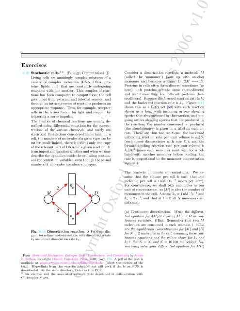
Fig. 8.11 Dimerization reaction. A Petri net diagram
for a dimerization reaction, with dimerization rate
k b and dimer dissociation rate k u.
u
1 From Statistical Mechanics: Entropy, Order Parameters, and Complexity by James
P. Sethna, copyright Oxford University Press, 2007, page 178. A pdf of the text is
available at pages.physics.cornell.edu/sethna/StatMech/ (select the picture of the
text). Hyperlinks from this exercise into the text will work if the latter PDF is
downloaded into the same directory/folder as this PDF.
2 This exercise and the associated software were developed in collaboration with
Christopher Myers.
1
D
Consider a dimerization reaction; a molecule M
(called the ‘monomer’) joins up with another
monomer and becomes a dimer D: 2M ←→ D.
Proteins in cells often form dimers; sometimes (as
here) both proteins are the same (homodimers)
and sometimes they are different proteins (heterodimers).
Suppose the forward reaction rate is k d
and the backward reaction rate is k u. Figure 8.11
shows this as a Petri net [50] with each reaction
shown as a box, with incoming arrows showing
species that are consumed by the reaction, and outgoing
arrows showing species that are produced by
the reaction; the number consumed or produced
(the stoichiometry) is given by a label on each arrow.
There are thus two reactions: the backward
unbinding reaction rate per unit volume is k u[D]
(each dimer disassociates with rate k u), and the
forward binding reaction rate per unit volume is
k b [M] 2 (since each monomer must wait for a collision
with another monomer before binding, the
rate is proportional to the monomer concentration
squared).
The brackets [.] denote concentrations. We assume
that the volume per cell is such that one
molecule per cell is 1 nM (10 −9 moles per liter).
For convenience, we shall pick nanomoles as our
unit of concentration, so [M] is also the number of
monomers in the cell. Assume k b = 1 nM −1 s −1 and
k u = 2 s −1 , and that at t = 0 all N monomers are
unbound.
(a) Continuum dimerization. Write the differential
equation for dM/dt treating M and D as continuous
variables. (Hint: Remember that two M
molecules are consumed in each reaction.) What
are the equilibrium concentrations for [M] and [D]
for N = 2 molecules in the cell, assuming these continuous
equations and the values above for k b and
k u For N = 90 and N = 10 100 molecules Numerically
solve your differential equation for M(t)
Copyright Oxford University Press 2006 v1.0

2
for N = 2 and N = 90, and verify that your solution
settles down to the equilibrium values you
found.
For large numbers of molecules in the cell, we expect
that the continuum equations may work well,
but for just a few molecules there surely will be relatively
large fluctuations. These fluctuations are
called shot noise, named in early studies of electrical
noise at low currents due to individual electrons
in a resistor. We can implement a Monte
Carlo algorithm to simulate this shot noise. 3 Suppose
the reactions have rates Γ i, with total rate
Γ tot = ∑ i
Γi. The idea is that the expected time
to the next reaction is 1/Γ tot, and the probability
that the next reaction will be j is Γ j/Γ tot. To simulate
until a final time t f , the algorithm runs as
follows.
(1) Calculate a list of the rates of all reactions in
the system.
(2) Find the total rate Γ tot.
(3) Pick a random time t wait with probability distribution
ρ(t) = Γ tot exp(−Γ tot t).
(4) If the current time t plus t wait is bigger than
t f , no further reactions will take place; return.
(5) Otherwise,
– increment t by t wait,
– pick a random number r uniformly distributed
in the range [0, Γ tot),
– pick the reaction j for which ∑ i