Surnames and a Theory of Social Mobility - University of Chicago ...

Surnames and a Theory of Social Mobility
Gregory Clark, University of California, Davis
gclark@ucdavis.edu, March 25, 2013
Using the information content of surnames to measure social
mobility, it is shown that the true intergenerational correlation of
social status is in the order of 0.7-0.8, much higher than is estimated
by conventional methods. This intergenerational correlation is
similar across dramatically different societies: medieval England,
modern England, pre-industrial Sweden, modern Sweden, the USA,
Quing and Communist China, Meiji and modern Japan, and Chile.
Surnames also show mobility to follow a simple law-like process
across many generations. One simple Law of Motion seems to
capture all social mobility. In this paper I offer a theory as to why
these measures differ from conventional mobility estimates. I also
argue that the nature of the process suggests biological inheritance of
abilities, as opposed to intergenerational capital transfers, is the main
determinant of social position.
Introduction
This paper summarizes the results of Clark, 2012, 2013, Clark et al., 2012, Clark
and Cummins 2012, 2013, Clark and Ishii, 2012, Clark and Landes 2013, and Hao
and Clark, 2012, which examine social mobility rates over many generations, across
countries, and across different measures of social status, using the information
content of surnames. The framework adopted is very simple. We assume that we
have measures of status that are cardinal, or can be approximated as cardinals:
earnings, income, wealth, years of education, level of education, occupational status,
or longevity. Then if y t is this status measure (or in the case of income or wealth its
logarithm), and is normalized to have a constant standard deviation and a mean of 0,
the intergenerational correlation of y, β, is inferred just as the regression coefficient
from
(1)

1-β is the rate of regression to mean. β 2 is share of social position variance derived
by inheritance. If the process of transmission of status is Markov, then β n is the
intergenerational elasticity of status over n generations.
There have been over the last 40 years many measures of the intergenerational
correlation of various measures of status within this framework, looking just at two
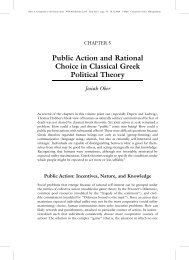
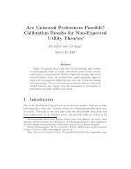
generations. Figure 1, for example, shows estimates of the intergenerational elasticity
of earnings for a variety of countries summarized by Corak, 2011. Figure 2 shows
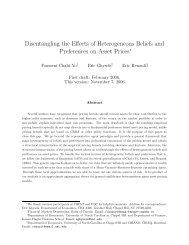
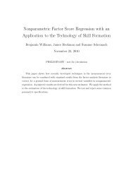
equivalent intergenerational correlation for years of education by Hertz et al., 2011.
These studies suggest the following conclusions.
Intergenerational correlations are typically of the order of 0.2-0.5 for income,
years of education, occupational status, and even for wealth.
Social mobility rates vary substantially across countries. In particular the
more unequal is a society in income the lower are mobility rates.
Social mobility rates vary substantially across different measures of status
such as earnings and education within the same country.
The
intergenerational elasticity for earnings in Scandinavia is consistently lower,
for example, than that for education.
Thus mobility rates are “too low” in some societies. With better
opportunities for the children of low income or status families, more
mobility would be possible.
If status transmission is Markov, earnings, occupational, and social mobility
are all largely complete within 2-5 generations. The descendants of a person
with an income 20 times above the average, or 1/20 of the average, 5
generations later will have expected incomes within 10% of the average.
If the process is Markov, and the variance of status across generations is
constant, then the fraction of variance of social position explained by
inheritance is low. The above figures suggests this is 4% in Scandinavia, and
22% in the USA. Most of social status is not predictable at birth.
Recent studies of multiple generations consistently suggest, however, that the
process is not Markov. If we estimate
y t+1 = β 1 y t + β 2 y t-1 + β 3 y t-2 + u t
then b 2 >0, b 3 >0 and so on. Even controlling for parents, the status of
grandparents, and even great-grandparents is predictive of this generation’s
status (Lindahl et al., 2012, Long and Ferrie, 2012).

Education Correlation - b
Earnings Correlation
Figure 1: Intergenerational Earnings Correlations and Inequality
0.8
0.7
0.6
0.5
0.4
0.3
0.2
0.1
Sweden
Norway
India
NZ
Japan
Finland
Canada
Source: Corak, 2012, Figure 2. Canada, personal communication from Miles
Corak. India from Hnatkovska et al., 2013.
UK
China
USA
Peru
Argentina
Chile
0
0.1 0.2 0.3 0.4 0.5 0.6
Gini Coefficient Income
Figure 2: Intergenerational Education Correlation and Inequality
0.7
Peru
0.6
Brazil
Italy
0.5
USA
0.4
Norway
0.3 Denmark UK
Sweden
0.2
0.1
0
0.2 0.3 0.4 0.5 0.6
Gini Coefficient Income
Sources: Hertz et al., 2011, table 2. Gini for Income, World Bank.

However, when we switch to measuring intergenerational correlations through the
rate of regression to the mean of social groupings identified by surnames we find the
following. Denoting the intergenerational correlation measured in this way as b we
find:
o Persistence, b, is much higher than conventionally measured for all aspects of
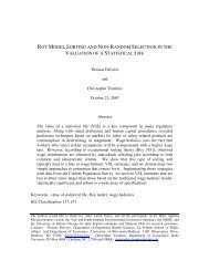
status. Table 1 and figure 3 shows for various periods and countries
estimates of persistence through surnames. The typical value is 0.7-0.8.
Complete regression to the mean takes 10-16 generations, 300-500 years.
o The rate of persistence is similar for education, occupation and wealth. It is
similar across the entire distribution of status, being the same for the upper
tail as for the lower tale.
o The rate of persistence varies little between societies and epochs. There is
little sign that rates of social mobility are “too low” in some societies.
o Regression to the mean measured in this way is indeed Markov. The social
status of the next generation is predicted only by the status of the current
generation.
o Since b 2 = 0.5-0.65 the majority of social status is determined at conception.
o We observe persistent elites and underclasses only in two cases. The first is
an isolated elite with marital endogamy (as with Hindu castes in India,
Muslims in India, or the Copts in Egypt, or Christians elsewhere in the
Muslim world). The second is where an elite or an underclass is maintained
by selective retention of members with the elite or underclass characteristics,
and recruitment of outsiders with the characteristic.
o Assortative mating is what makes b so high. Mating has become more
assortative in the modern world, so mobility rates may decline further
(Herrnstein-Murray claim).
o The fact that regression to the mean does not occur when societies have
completely endogamous marriage, and the failure of social institutions to
have any systematic effects on mobility rates, suggests that social mobility is a
largely biological process.

Table 1: Estimates of b from Surnames
Country Measure Period Intergenerational
Correlation
MODERN
USA Attorneys 1950-2011 0.83-0.94
USA Doctors 1950-2011 0.73-0.80
England Attorneys, Doctors 1950-2012 0.69-1.00
England Wealth 1950-2012 0.74
England Education 1950-2012 0.80
Sweden Education 1950-2011 0.65-0.88
Sweden Attorneys, Doctors 1950-2011 0.70
Chile Occupations 1940-2010 0.83
China Education 1950-2011 0.66-0.92
Japan Education 1950-2012 0.84
India Doctors 1950-2009 0.89
HISTORIC
England Wealth 1650-1850 0.71-0.85
England Wealth 1380-1650 0.74-0.85
England Education 1200-1500 0.80-0.90
England Education 1500-1800 0.80-0.90
Sweden Education 1700-1900 0.75-0.88
Sweden Doctors 1890-1950 0.70
India Doctors 1860-1950 0.89
Japan Education 1880-1900 0.72
China Education 1700-1900 0.81
Sources: England, Clark, 2013, Clark and Cummins, 2012, China, Hua and Clark, 2012,
India, Clark and Landes, 2012, Japan, Clark and Ishii, 2012, USA, Clark et al., 2012. Chile
communication from Daniel Diaz.

Intergenerational Correlation
Figure 3: Conventional versus Surname estimates of Status Persistence, 1950-2012
1
0.8
0.6
0.4
0.2
0
Why are these results so different from the conventional studies One
suggestion is that by looking at surname groupings we are implicitly controlling for
errors in the measurement of current status that will reduce the estimated
intergenerational correlation β, so estimating higher values for b. But the correlation
estimates in figure 1 are those corrected for measurement error. And in the case of
education in figure 2 measurement errors are believed to a relatively insignificant.
The different bs estimated in these ways are not about different degrees of control
for measurement errors.
The resolution proposed here that individuals and families have some
underlying general level of social status in generation t, x t , where x t is always
regressing toward the mean across generations to that
(2)
where x t and x t+1 are assumed to have a mean of 0, and a constant variance
x is normally distributed.
., and

However, we do not typically directly observe the complete social status of
families, but some partial measure, y t , where such measures would be earnings,
wealth, years of education, educational status, or occupational status. For each
generation t
(3)
where u t is a random component linking the underlying status of the family to the
particular observed measure of status.
The random component linking aspects of social status to underlying social
status exists for two reasons. First there is an element of luck in the status attained
by individuals given their underlying competence. If we look at earnings, people
happen to choose a successful field to work in, or a successful firm to work for.
They just succeed in being admitted to Harvard, as opposed to just failing. They
marry a supportive spouse, or end up instead shackled to a needy partner. But,
second, people trade off income and wealth for other aspects of status. They choose
a career as a philosophy professor as opposed to a lower occupational status, but
more lucrative career, as a plumbing hardware salesman.
The above implies that the conventional studies of social mobility, based on
estimating the β in the relationship
(1)
will underestimate the true b linking underlying social status across generations. In
particular the expected value of β will be not be b, but instead θb, where θ

use here over multiple generations, even when they are based on partial measures of
social mobility such as educational or occupational status, will closely approximate to
the true underlying b. This is because by aggregating over groups of individuals with
the same surname we can make the error component linking observed status y and
underlying status x go to zero.
Evidence of the loose connection of the various single aspects of status for
single individuals is easy to find. Table 2 shows a summary of these correlations for
the following aspects of status: academic aptitude (typically IQ), occupational status,
education, earnings, and wealth. The correlations for any two attributes average only
around 0.43. That means, for example, that if I know the academic aptitude (IQ) of
my child I can typically predict less than a fifth of the variation in possible
educational achievement, occupational status, earnings, or wealth. 1 This loose
association for a person of the various aspects of status means that each aspect in
general will have to also be weakly correlated across generations. But, the argument
is, if we were to take the broadest possible measure of the aggregate status of an
individual, that would be closely correlated across generations.
The one generation studies, as long as the particular aspect of status, y, is
correctly measured, will indeed report what good estimates of what the correlation is
across one generation, for any particular aspect of status. There is nothing
intrinsically wrong with these estimates. However, the mistake is to infer from these
studies that overall status regresses to the mean anything like as rapidly.
This simple switch in thinking about the mechanism of social mobility produces
a number of testable predictions.
1 Bowles and Gintis, 2002, point out this loose association between IQ and other social
outcomes creates puzzles about how these other attributes are inherited as strongly as they
are. IQ inheritance cannot be the primary pathway.

Table 2: Correlations between the Aspects of Status, Individuals
Status Element
Mental
Education Occupational
Earnings
Wealth
Aptitude
Status
(IQ etc.)
Mental Aptitude - .45-.62 1 .16-.31 2 .23-.30 3 .16 4
Education - - .41-.85 5 .32-.34 6 .22-.38 7
Occupational status - - - .34-.71 8 .13-.34 9
Earnings - - - - .60-.61 10
Sources: 1Scarr and Weinberg, 1978, Husén, 1991, Zagorsky, 2007. 2Cagney and
Lauderdale, 2002, Hauser, 2002, Griliches, 1972. 3 Griliches, 1972, Zagorsky, 2007, Zax et
al., 2002. 4 Zagorsky, 2007. 5 Scarr, 1981, Hauser and Warren, 2008, Pfeffer, 2011. 6 Cagney
and Lauderdale, 2002, Griliches, 1972, Pfeffer, 2011. 7 Cagney and Lauderdale, 2002, Pfeffer,
2011. 8 Griliches, 1972, Hauser and Warren, 2008 (wages). 9 Pfeffer, 2011. 10 Budria et al.,
2002, Hendricks, 2007.
1. The observed rate of regression to the mean of individual aspects of status
will be determined by how well they are predicted by the underlying status of
families. The lower their correlation with this underlying status the less
intergenerational connection there will seem.
2. In the long run all aspects of status will regress to the mean at the same rate.
Underlying mobility measured through earnings, wealth, education, or
occupational status will be the same. There will be a stable correlation
between aspects of status
3. The underlying process of social mobility will be Markov. It will proceed at
the same rate across all generations.
4. Social groups, such as in the USA such as Jews, Blacks, Latinos and Native-
Americans, will appear to have lower rates of social mobility than the general
population on conventional measures, but will in fact exhibit the same rate of
regression to the mean as the society as a whole.

What causes the conventional measures to overestimate underlying social
mobility rates is the presence of the error term, e, linking partial measures of status
with underlying competence. However, when we look at groups of people, as long
as they are grouped by identifiers that do not correlate with this error term, such as
race, religion, national origin, or even, as we shall see, common surnames, then by
averaging across people we reduce this error term. While
y i = x + u i (3)
at the individual level, at the group level,
̅ ̅ .
Now the ̅ accurately tracks ̅ without the intrusion of the errors, and we can
correctly estimate social mobility just from observed partial measures of this.
Thus when we look at such groups of individuals the underlying slow rate of social
mobility becomes apparent, even when we only have the usual partial indicators of
underlying social competence. Table 3 thus shows for the US the effects including
separate intercept terms for Blacks, Latinos and Jews in estimating the
intergenerational elasticity of family income in the US for a sample of 3,568 parental
incomes in 1967-71, and the income of adult children in 1994-2000.
The regression estimates imply that, even when we control for all other
measured attributes of parents in 1967-71 such as education, occupation, and
household cleanliness, we can predict that Black, Latino and Jewish families are all
regressing more slowly to the mean than is found for the population as a whole. 2
The Hertz interpretation is that this is because of special characteristics of these
groups. My interpretation, however, is that if we included a dummy for membership
in any high or low income group then it would have a significant coefficient also.
This is because the underlying rate of regression to the mean for all families is much
2 Hertz, 2005.

Table 3: Regression to the mean controlling for race and religion, USA
Independent
Variable
No controls Only Race All Observable
Parental
Characteristics
Ln Family Income of
Parents
0.52** 0.43** 0.20**
Black - -0.33** -0.28**
Latino - -0.27** -0.15
Jewish - - 0.33**
Notes: ** = significant at the 1 percent level. Only 3 percent of the sample was
Latino.
Source: Hertz, 2005, table 6.
lower than the conventional regression estimates imply. Thus once we can identify
families as collectively belonging to groups of on average high or low incomes, we
can predict much better the expected income in the next generation.
This same effect of group background was found by George Borjas in his study
of immigrants where he regressed
̅
where y was log wage or years of education, i indexed families, j the country of origin
of fathers, and t the generation (Borjas, 1995). ̅ was the average log wage or years
of education of all men from that country, estimated from the 1980 census reports of
education and occupation. In both the case of education and earnings the average
status of people from the country of origin was predictive of the outcome for sons
(b 0 +b 1 equalled 0.44 for education and 0.70 for earnings) (Borjas, 1995, table 8).

Borjas interprets this as the result of “ethnic capital” externalities. Sons from
ethnic groups with high average education levels do better than would be predicted
from the education of the father alone, because of spillovers from the education of
others in the community. But again our interpretation would be that there is likely
little or no externality. It is just that information on the country of origin allows a
better prediction of the likely “true” underlying status of families, and so a better
prediction of the son’s outcomes. That is why the same effect appears below for the
wealthy of 1923-4 in the USA, who span many ethnic communities.
This simple understanding of social mobility can resolve more than the puzzles
of group status persistence. For it can also explain the connection detailed in figure
1 between income mobility rates across countries and the inequality of income. The
greater are the random components in determining measures of status such as
income, relative to the systematic elements stemming from underlying status, the
greater will be the degree of mismatch between such partial one generation estimates
of regression to the mean, and the underlying regression of fundamental social
status.
The USA, for example, has much greater inequality in earnings than does
Sweden. Figure 4 shows, for example, the salaries in $2010 for some comparable
high and low status occupations in Sweden and the USA. A US doctor earns six
times the wage of a bus driver, while in Sweden the ratio is only 2.3 times. A US
professor earns sixty percent more than a bus driver, in Sweden it is only forty
percent more.
We can represent this by modifying equation (3) above to
y t = ψx t + u t
where the ψ linking social competence to earnings is higher in the US than in
Sweden. ψ in the US could be as much as twice the ψ in Sweden. This implies that
the proportion of variation in earnings in the USA that is explained just by random
factors is lower. This will mean that the downwards bias in estimates of social
mobility coming from earnings will be lower in the US. Thus the US will appear,
because of greater wage inequalities, as more immobile across generations than
Sweden. Just the greater wage inequality in the US can easily double the measured
intergenerational correlation if the true intergenerational correlation of status is 0.75.

Figure 4: Average Earnings by Occupation, Sweden and the USA, 2008
$
200,000
160,000
120,000
80,000
40,000
0
USA
Sweden
Sources: USA – Bureau of Labor Statistics, National Occupational Employment and Wage
Estimates, May 2010. Sweden – Statistics Sweden, Wage and salary structures, private sector
(SLP), 2011.
This explanation can also explain why the proposition that as earnings inequality
has increased in the past forty years in the USA, social mobility rates have declined, is
wrong. 3 All that is happening is that the standard measures of mobility now more
accurately reflect the underlying mobility rates.
This simple model also explains another puzzle of conventional mobility
estimates, the stronger than expected correlation of social status between
grandparents and grandchildren, and great-grandparents and great-grandchildren. 4
For this model contains the prediction that after the second generation, measured
social mobility rates will slow down to the underlying mobility rate of social
competence. Measured downwards mobility for a high income family will be fast in
3 Though this notion has gained popular currency (see, for example, Foroohar, 2011) there
seem to be no academic studies suggesting it.
4 See, for example, Long and Ferrie, 2013. Lindahl, et al., 2012.

the generation of the children, but then much slower for the generation of the
grandchildren, the great-grandchildren and so on measured relative to the first
generation.
The link between children and parents, the β normally estimated, will relate to
the underlying persistence of status in the form
̂
where φ is the attenuation factor caused by the random components linking
observed status on any one dimension with underlying status. When we look,
however, at the correlation between grandparents and grandchildren, and estimate
now ̂, the correlation across two generations, we will find that it is not ̂
as would be expected from simple models of social mobility, but instead
. The
downward bias caused by the error component in the measure of status is the same
across all generations. Thus if ̂ , then ̂ will not be the 0.14
expected on conventional mobility estimates, but double the size at 0.28.
There is data on the intergenerational correlation of education and earnings,
estimated from occupations, for four generations of families in Malmo, Sweden
which allow us to test this claim. Table 4 shows the correlations in years of
education across generations. The one generation correlation averages 0.35.
The bottom panel in the table now shows what the estimated ̂ s would be if
the underlying rate of persistence for status is actually double this at 0.7, but there is
an attenuation factor of 0.5. This produces predicted correlations for the educational
status of grandchildren and great-grandchildren that are a bit on the high side
compared with the actual results, but the difference is not statistically significant.
The underlying b that would best fit this pattern of intergenerational correlations
would be b = 0.61, still substantially higher than the observed correlation of 0.35
between adjacent generations.
Thus we see that in all these cases that represent anomalies for the standard
estimates of fast social mobility, the simple alternative model of a much slower
underlying rate of mobility for a deeper, unobserved, social competence can account
for the results.

Table 4: Persistence in Education Across Multiple Generations in Sweden
Last Generation
Great-
Grandparents
Grandparents
Parents
OBSERVED
Grandparents 0.334
Parents 0.229 0.312
Children 0.123 0.202 0.412
PREDICTED, b = 0.7
Grandparents 0.334
Parents 0.226 0.312
Children 0.173 0.253 0.412
Source: Lindahl et al., 2012, table 2.
Another feature of conventional estimates of social mobility is that the
suggested rates of mobility for different characteristics are different. Cognitive
abilities in Sweden, for example, are found to be strongly correlated across
generations, with a β of 0.77. But at least in Scandinavia income and educational
attainment have a much lower hereditability, with βs of 0.2 to 0.3.
Suppose, for example, that we began with a Swedish elite that was distinguished
by high cognitive abilities. Since cognitive abilities are correlated with income and
educational attainment this group would also be distinguished on these dimensions.
But they would be less distinguished, since the correlation between cognitive abilities
and income or educational attainment is no more than 0.5. However, within a few
generations the descendants of this group would have regressed to the mean in terms
of income and educational attainment.
Since the regression to the mean of cognitive abilities is so much slower,
however, they would still be distinctive in this dimension. So we would have a group

of people with a factor that normally predicts both higher earnings and educational
attainment, yet with average attainment in both these respects. This seems a
troubling implication of current estimates of social mobility for different aspects of
social status.
In contrast the model of one underlying measure of social competence that is
suggested here would predict that the families scoring highly on this underlying
measure, the regression to the mean would be the same for all aspects of status:
cognitive abilities, non-cognitive abilities, earnings, wealth, education, occupations
and longevity. The different rates of mobility seen on this individual measures
reflects just how much random component there is linking them to underlying social
competence.

Surnames
To investigate the rate of regression to the mean of this deeper underlying social
status (and by implication the long run rate of regression to the mean of income,
wealth, occupational status and education) this study traces people not through
individual family linkages, but through surnames over multiple generations.
In many societies surnames are inherited unchanged from one generation to the
next, typically through the patriline. If at some generation surnames differ in social
status, we can then trace through surnames the descendants of the current
generation for many generations. As long as there is nothing peculiar about the path
of descent of surnames, the surnames link the status of groups of families many
generations in the past with their descendants in the present. 5
When initially formed, surnames in many societies were associated with social
status. For example, in England some high status land owners already possessed
surnames at the time of the Domesday Book of 1086, which listed the major
landholders of England. Most of these people were the Norman, Breton and
Flemish followers of Duke William of Normandy, who seized the throne of England
in 1066. These surnames thus constitute a distinctive subset of modern English
surnames: Baskerville, Beaumont, D’Arcy, de Vere, Mandeville, Montgomery,
Vernon, and Villiers, for example. In England also about 10 percent of surnames
derive from the occupations of the original holder, and these occupations had a
range of social statuses: Smith, Baker, Shepherd, Clark, Chamberlain, Butler.
In Sweden, surnames started as patronyms which changed with each generation.
Sven, son of Lars, was Sven Larsson. But his son Gunnar would be Gunnar
Svensson. For the ordinary people patronyms did not become fixed across
generations until the late nineteenth century. However, from at least the 17 th century
two groups of high status individuals were acquiring permanent and distinctive
surnames. The first were those who attended universities, who adopted latinized or
grecified surnames such as Celsius, Linnaeus, and Melander. The second was the
aristocracy, often imported mercenary commanders, who imported surnames from
5Olivetti and Paserman, 2012, find that there is no difference in the occupational status of
sons-in-law compared to sons in the USA 1850-1930, so that there is no sign that the social
mobility along the patriline is any slower than in the matriline.

Germany, Scotland and elsewhere or created their own distinctive family names
when inducted into the house of nobles such as Leijonhufvud.
Even in societies such as England where the early introduction of universal
surnames by 1300 meant that by 1800 common surnames all had the same average
social status, we can study modern long run social mobility through the use of rare
surnames. Through processes of chance in each generation some such rare
surnames will be on average of high status, others of low status. If in some initial
generation, surnames are predictive of social status, then over time, as long as b is
less than 1, surnames should lose this information. And the rate at which they lose it
is a measure of the rate of social mobility. If the high rates of mobility typically
found in one generation studies are predictive of long-run rates of social mobility,
then within a few generations surnames should contain no systematic information on
social status.
The crucial advantage the surname linkages give is that we can identify high and
low status groups in some initial period, and then track them over multiple
generations using their initial classification of status into high and low groups. This
means that after the first generation the average error from the underlying status
associated with each surname group in each generation is 0, so that for the surname
cohorts
b y = b x
where x is the underlying broader social status of families or groups.
The b x estimated for surnames, however, is not identical to that within families,
if we could estimate that. This is because in surname cohorts, when we estimate
̅ ̅ (4)
̅ measures, for example, the average log wealth across a group of people with the
surname k in the initial generation. But some of these people will not have any
children, and would not be included in the within family regression. And those with
1 child from generation t get weighted as much as those with 10 children. Thus
surname cohorts themselves introduce some measurement error in y t , which will
reduce the observed value of b. The magnitude of this downwards bias will decline,
however, the larger the size of the surname groupings unless there is some systematic
connection between social status and child numbers.

In the years 1890-1980 fertility was consistently higher for lower status families
in countries such as the USA, England, and Sweden. In this case the surname
estimate of b will be biased towards 0 for elite surnames, and away from 0 for
underclass surnames in these years. In the years before 1800 in England and Sweden
fertility was substantially higher for upper class groups. Thus for elite surnames in
the pre-industrial world, the estimate of b will be biased upwards, and for underclass
groups biased downwards. We shall see below that for some groups, this
demographic bias can be so strong that a surname will appear to be moving away
from the mean.
In looking at social mobility through surnames in some cases we have direct
measures such as wealth in England 1858-2012 (Clark and Cummins, 2012). Then it
is easy to estimate b from the equation
̅ ̅ ̅ ̅
where ̅ is the average log wealth at death of surname group R, and ̅ is the
average wealth at death of England as a whole. Figure 5 shows this information for
England for three initial rare surname groups: wealthy surnames at death 1858-87,
prosperous surnames at death 1858-87, and poor surnames at death 1858-87. A
sample of the surnames used are shown in table 5, labelled just as samples A, B and
C. These surnames are rare enough that the surnames themselves are not doing any
work in slowing the regression to the mean. Thus most people reading this will not
be able to discern which surnames belonged to the rich, prosperous and poor
samples. 6
Table 6 shows the average implied estimate of b for each period, and across the
5 generations as a whole. Since the poor group is much closer to average wealth
than the two richer groups, the b estimate here is much noisier, as can be seen in the
variance of the estimates in the last row of table 6. Looking at the top two wealth
groups we see quite stable average estimates of b across the 5 generations - 0.75,
0.66, 0.73, and 0.74 – for an overall average of 0.72.
6 Sample A is the rich, B the poor, and C the prosperous.

ln Wealth - Ave. ln Wealth
Figure 5: Log Average Wealth relative to the Average, 1858-2011
6
5
4
3
2
Rich
Poorer
Prosperous
1
0
1860
-1
1890 1920 1950 1980 2010
-2
Table 5: Rare English Surname Samples, 1858-1887
Sample A Sample B Sample C
Ahmuty Aller Agace
Allecock Almand Agar-Ellis
Angerstein Angler Aglen
Appold Anglim Aloof
Auriol Annings Alsager
Bailward Austell Bagnold
Basevi Backlake Benthall
Bazalgette Bagwill Berthon
Beague Balsden Brandram
Berens Bantham Brettingham
Beridge Bawson Brideoake
Berners Beetchenow Broadmead
Bigge Bemmer Broderip
Blegborough Bevill Brouncker
Blicke Bierley Brune

Table 6: b Values Between Death Generations
Generation Rich Prosperous Rich and
Prosperous
Poor
1888-1917 0.66
(0.026)
0.86
(0.052)
0.75
(0.028)
0.66
(0.061)
1918-1959 0.68
(0.031)
0.64
(0.041)
0.66
(0.030)
1.12
(0.136)
1960-1987 0.73
(0.040)
0.74
(0.051)
0.73
(0.035)
0.30
(.076)
1999-2011 a 0.70
(0.098)
0.80
(0.125)
0.74
(0.078)
0.41
(0.615)
Average 0.69 0.76 0.72 0.61
Notes: Bootstrapped standard errors in parentheses. a The ̂ reported here is the
estimated ̂ multiplied by 0.94 of to reflect that the generation gap here is only 23
years, because of the truncated generation.
However, in most cases we have instead measures of the fraction of people
bearing a surname who are in high or low status occupations over many generations
compared to the fraction of those surnames in the general population: university
graduates, doctor, attorney, member of Parliament, professor, author, or criminal.
To extract implied bs for these cases we proceed as follows. Define the relative
representation of each surname or surname type, z, in an elite group as
With social mobility any surname which in an initial period has a relative
representation differing from 1 should tend towards 1, and the rate at which it tends
to 1 is determined by the rate of social mobility.

To extract implied bs from information on the distribution of surnames among
elites we proceed as follows. Assume that social status, y, follows a normal
distribution, with mean 0 and variance . Suppose that a surname, z, has a relative
representation greater than 1 among elite groups. The situation looks as in figure 6,
which shows the general probability distribution function for status (assumed
normally distributed) as well as the pdf for the elite group.
The overrepresentation of the surname in this elite could be produced by a
range of values for the mean status, ̅ , and the variance of status, , for this
surname. But for any assumption about ( ̅ , ) there will be an implied path of
relative representation of the surname over generations for each possible b. This is
because
̅
̅
Also since ,
With each generation, depending on b, the mean status of the elite surname will
regress towards the population mean, and its variance increase to the population
variance (assuming that < ). Its relative representation in the elite will decline
in a particular pattern.
Thus even though we cannot initially fix ̅ and for the elite surname just
by observing its overrepresentation among an elite in the first period, we can fix
these by choosing them along with b to best fit the relative representation of the elite
surname z in the social elite in each subsequent generation. In practice it turns out
to matter little to the estimated size of b in later generations what specific initial
variance is assumed. Below we assume that the initial variance of the elite surname
status is the same as the overall variance, since this assumption fits the observed time
path of relative representation well in most cases. In the case of the wealth of the
deceased in England figure 7 shows that for the wealthier surname probated it was actually
more dispersed than for the population as a whole. But it does show the pattern
premised in figure 6 of a rightward shift to the whole distribution.

Density
Relative Frequency
Figure 6: Regression to the Mean of Elite Surnames
All Surnames
Elite Surnames
All - Probated Limit
ln Wealth
Figure 7: Wealth Distribution of Probated, Rich, Prosperous and Brown
Surnames, 1918-1959
0.30
0.25
Brown
Prosperous
Rich
0.20
0.15
0.10
0.05
0.00
-7.7 -5.3 -3.7 -2.5 -1.8 -1.2 -0.5 0.1 0.7 1.4 2.0 2.7 3.3 3.9 4.6 5.2 5.9 6.5 7.1 7.8 8.4 9.0 9.6 10.3 10.9
Ln Wealth - average ln Wealth

Table 7: Share Probated by Generation, England 1858-2012
Period
All Deaths
21+
Rich
1858-87
Prosperous
1858-87
Poor
1858-87
1858-87 0.15 0.84 0.57 0.00
1888-1917 0.22 0.68 0.54 0.10
1918-52 0.38 0.73 0.63 0.21
1953-89 0.46 0.70 0.65 0.34
1990-2011 0.43 0.61 0.59 0.37
For England in 1858-2012 average wealth at death is determined by the average
estate value of those probated as well as the fraction of people probated. Table 7
shows this fraction for all adults (21 and over at time of death) by generation in
England 1858-2012, as well as for those in the three rare surname groups of 1858-87.
As can be seen the rich surnames continue to be probated at higher rates than the
general population even into the last generation, 1990-2012. The poor group of
surnames in 1858-87 is always probated at lower rates than the general population.
By dividing the probate rate of each group in each period by the general probate
rate we can calculate the relative representation of each surname group among the
probated. This is shown in table 8. Thus in 1858-87 the rich surnames were 5.5
times as likely to be probated as the average person at death. Assuming wealth
variance for each surname equal to the social average we then get an implied
persistence rates across generations, b, shown in table 9. 7
7 For the poor surnames we cannot derive this for the first period since by construction noone
in this surname group was probated in this period. With a normal distribution of wealth
in each period it would not be possible to have a 0 percent of any group probated.

Table 8: Relative Representation by Generation
Period
All Deaths
21+
Rich
1858-87
Prosperous
1858-87
Poor
1858-87
1858-87 1.00 5.48 3.71 0.00
1888-1917 1.00 3.10 2.46 0.48
1918-52 1.00 1.92 1.65 0.56
1953-89 1.00 1.51 1.39 0.73
1990-2011 1.00 1.42 1.37 0.87
Table 9: Estimated b by Surname Group and Period, Probate Shares
Period
Rich
1858-87
Prosperous
1858-87
Poor
1858-87
1888-1917 0.63 0.81 0.37
1918-59 0.75 0.65 1.04
1960-93 0.59 0.70 0.80
1994-2011 a 0.78 0.81 0.05
Average 0.69 0.75 0.57
Direct Estimate 0.69 0.76 0.61
Note: a b estimate adjusted down to reflect incomplete generation observed.
The estimated intergenerational correlation of wealth from just the fractions of
people in each surname group probated is very similar to that estimated directly by
calculating average log wealth, as is also shown in table 9. Thus though in most cases
we only observe the status of social groups by observing their relative representation
in some top x% of the population, the estimates derived in this way will be
completely comparable with the standard estimates.

Intergenerational Correlations by Country and Status Type
England
The tables below report the various intergenerational correlations found in the
studies of the various countries. Table 9, for example, shows the various estimates
of b for England, running from 1200 to 2012, and covering wealth, education,
occupations, and membership in the political elite. These estimates all suggest high
intergenerational correlations of status, on all measures. There is no clear sign of an
increase in social mobility over time.
For wealth, for example, I have measures of probate rates from 1380 to
2012. We see above that for rare surname groups we get an estimated b of 0.74 for
1858-2012. We can follow the probate rates of these same surnames back to 1680
and get a measure of b for 1680-1858. The model posited above that underlying
status is linked across generations by the formula
also has implications about what the path of relative representation will be for
surnames observed to be elite in any specific generation in the periods before that
observation. The OLS estimator of b in this expression is
Suppose we were instead to posit that
̂
∑
∑
The OLS estimator of β would then be
̂
∑
∑
If the variance of x t is the same as that of x t+1 , then it will also be the case that
. Since we have normalized variance to be the same in each generation

we have met this condition. Thus the rate of rise of surnames to be an observed elite
in any generation should mirror their rate of decline back to mediocrity.
Table 9: b Estimates for England
Period Wealth Education Occupations Political Elite
1200-1400 - 0.80-0.86 - 0.91
1400-1650 0.74-0.85 0.77-0.86 - 0.91
1650-1850 0.71-0.85 0.77-0.83 - 0.91
1850-1950 0.70 0.77-0.83 - 0.81
1950-2012 0.74 0.80 0.65-1.00 -
Figure 8: The Prehistory of the Rich and Poor of 1858-87
8.00
4.00
b = 0.85
2.00
1.00
1680 1710 1740 1770 1800 1830 1860
0.50
0.25
0.13
b = 0.71
Note: The upper curve is the rare rich surnames of 1858-87, the lower curve the rare poor
surnames of 1858-87.

This is exactly what we observe in figure 8. The rare surnames of the rich in
1858-1887 rise in their status 1680-1858, those of the poor decline in status. The
implied b for the rich from the rate of rise is 0.85, that of the poor from the rate of
decline 0.71.
Earlier we can estimate b from the decline in relative representation among
probates of 13 th century elite surnames, locative surnames for example, or the rise of
surnames earlier concentrated in the center of the status distribution, such as those
of artisans. This produces moderately higher estimated levels of b 1380-1858, in the
range 0.74-0.85. But before 1538 there is uncertainty about the population stock of
surnames needed to calculate these persistence rates.
The continued high level of persistence of wealth in the modern period is
surprising given the changes in the tax treatment of inheritances over the last
hundred years in the UK. As figure 9 shows, before 1878 inheritance taxes were
modest. Indeed for most of the period before 1800 there were no taxes on
inheritances. But in the years 1946-1980 larger inheritances were taxed at rates of
75-80%. Thus we would expect that transfers of wealth between generations were
correspondingly reduced substantially for richer families in some recent generations.
Yet this seems to have had minimal effects on the persistence of wealth.
For education we can similarly estimate b over many generations in England
using the relative representation of surnames in Oxford and Cambridge, the only two
English universities up until the 1830s. Figure 10, for example shows the relative
representation at Oxford and Cambridge, representing a 0.7% elite of educational
achievement in England all the way from 1500-2012, of two sets of rare surnames:
rare surnames of men born 1780-1809 dying wealthy 1858-87, and rare surnames of
someone attending Oxford or Cambridge 1800-29. For these surnames we calculate
the relative representation at the universities for the succeeding generations, 1830-
59,…2010-2. We can also calculate their relative representation in the preceding
generations, going all the way back to 1530-59.
The patterns in figure 10 are striking. Surnames associated with the rich are
always more overrepresented at Oxford and Cambridge than those associated with
people who happened to attend the universities 1800-29, in all subsequent or prior

Relative Representation
Top Tax Rate (%)
generations. In 1830-59, for example, the rich surnames were 54 times as frequent in
Oxford and Cambridge as in the general population, and the earlier Oxbridge
Figure 9: Maximum Inheritance Tax Rates, UK, 1825-2012
100
90
80
70
60
50
40
30
20
10
0
1825 1850 1875 1900 1925 1950 1975 2000
Figure 10: Relative Representation and Implied bs at Oxbridge, 1530-2012
64
32
16
b = 0.83
b = 0.82
8
4
2
b = 0.77
b = 0.77
1
1530 1590 1650 1710 1770 1830 1890 1950 2010
Note: The circles indicate the observations for the wealthy surnames, the squares those for
the rare surnames appearing at Oxford and Cambridge 1800-29.

surnames 34 times as frequent. But the rate of decline of the overrepresentation of
these surnames at the universities is similarly slow. It is so slow that even now in
2010-2, just knowing that a rare surname was on average wealthy at death 1858-87
tells us that it will be 6 times more likely to show up on the Oxbridge rolls than the
average English surname. Just knowing that a rare surname had at least one enrollee
at Oxbridge 1800-29 allows us to predict that it will still be 3 times as likely to appear
at the universities now as the average surname.
But the rate of decline for each group is constant. One b fits all generations.
The implied b measure of persistence for the rich surnames 1830-2012 is 0.82, while
for the 1800-29 universities cohort it is 0.77. The rise of these surnames is
symmetrical as predicted. The estimated b underlying that rise 1530-1799 is 0.83 for
the rich surnames, and 0.77 for the one that happen to appear at Oxford and
Cambridge 1800-29. This data thus strongly supports the assumption that the
process of social mobility is indeed Markov. One underlying equation of mobility
x t+1 = bx t + e t
describes mobility over multiple generations.

Sweden
Table 10 summarizes the surname estimates of social mobility rates for Sweden
1700-2012 from Clark (2012). These estimates are based on occupation and
education, using attorneys, doctors, university students and Academicians as
representatives of elite surname groups. Three features are notable. First these
mobility rates are very similar to those reported for England 1300-2012. Second the
rates do not seem to show any clear downwards trend in the modern era. Third, the
mobility rates for education and occupation seem similarly slow.
Figure 11 shows the details of relative representation of surnames in some of
the Swedish Royal Academies, the most elite fraction of the academic establishment.
Comprehensive membership lists are available for the Swedish Academy of Sciences
(founded 1739), the Swedish Academy of Music (1771), and the Royal Academy
(1786). Together these three academies have had 2,834 domestic members.
Figure 11 shows the relative representation of the surnames of the eighteenth
century elite – Latinized surname and the surnames of nobles - in these three
academies by 30 year generations starting in 1739-1769, and ending in 1980-2012. In
the earliest period such surnames made up half of the members of the academy. By
1980-2012 this had declined 4.1% of the Academies. But these surnames in 2011
were only 0.71% of the Swedish population, so they were still strongly
overrepresented in the Academies.
The small number of members compared to other groups we have looked at
means that in the latter years there is a lot of sampling error in terms of the
frequency of elite surnames. Taking these academies to represent the top 0.1% of
Swedish society the implied persistence b over these 273 years is 0.88. There is also
little sign of an increased rate of regression to the mean for the entrants to the
academies 1980-2012 compared to 1950-79. The estimated b for elite surnames is
still 0.84.
Figure 11 also shows the relative representation of Patronyms, lower class
Swedish surnames, in the Academies. Such surnames are of course still strongly
underrepresented, but they have shown a slow but steady convergence towards
proportional representation. However, the implied b is 0.87, close to that for the
elite surnames. Again we see the predicted symmetry in terms of rates of upwards

Relative Representation
Table 10: Summary b Estimates by Period, Sweden
Group 1700-1900 1890-1979 1950-2012
Attorneys - - 0.71
Physicians - 0.67 0.88
University Students 0.78 0.85 0.66
Academicians 0.89 0.75 0.84
Figure 11: Elite and Lower Class Surnames in the Swedish Royal Academies
64.00
16.00
b = 0.88
Elite
Fitted Elite
..son
Fitted ..son
4.00
1.00
1740 1770 1800 1830 1860 1890 1920 1950 1980 2010
0.25
0.06
b = 0.87
0.02
Cohort

and downwards mobility. However, there is a caveat that many people in Sweden
whose father had a patronym did not take their father’s name as an adult, and this
switching was likely selective. This would reduce the rate of measured upward
mobility.
USA, 1920-2012
To measure mobility in the USA we use five groups of surnames – Ashkenazi
Jewish (e.g. Katz), Black (e.g. Washington), New France (e.g. Gagnon), Rich Rare
Surnames of the 1920s (e.g. Roosevelt), and rare surnames appearing as students in the
Ivy League 1850 and earlier. 8 Only Black surnames of English origin were used, to
identify the domestic Black population. Figure 12 shows the relative representation
of these surnames among doctors registered by the AMA 1920-49, 1950-79, and
1980-2011. Jewish, Rich 1920s and Ivy League pre-1850 surnames are
overrepresented. Black and New France surnames underrepresented. We can thus
calculate implied persistence rates for each group by generation.
For all five surname groupings there is a general convergence towards a relative
representation among physicians of 1 between the last two generations observed.
But, as can be seen in the graph, and will be confirmed by the estimates of the
underlying b for each group, this is a slow process that will not be complete for
many generations for most of these surname groupings.
In the previous generation, from 1920-49 to 1950-79, both the Jewish and Black
surname groups move away from the mean. The cause of this in the case of the
Jewish surnames was the explicit policy of many US medical schools between 1918
and the 1950s to limit the number of Jewish students admitted. These quotas led to
a decline in the number of Jewish students in AMA approved medical schools
declining from 794 in the class of 1937 to 477 in the class of 1940. 9
8 Black surnames were those for which at least 89% of holders of the surname in 2000
declared their race as Black in the census.
9 Borst, 2002, 210. These quotas were progressively tightened across the 1920s and 1930s.
Thus, in one of the most dramatic cases Boston University Medical School cut Jewish
enrollment in 1929 from 48 percent, to 13 percent by 1934 (p. 208).

Relative Representation
Figure 12: Relative Representation by Surname Type by Generation
8
4
2
Jewish
Rich 20s
Ivy League
New France
Black
1
1930 1950 1970 1990 2010 2030
0.5
0.25
Only in the 1950s were these anti-Jewish quotas lifted. These policy shifts show
up in the AMA directory data. There is a substantial decline in Jewish surname
overrepresentation for doctors completing medical school between the 1930s and
the 1940s. In figure 3.9 below which looks at relative representation by decade from
the 1940s on we see a rise in Jewish relative representation among those graduating
from medical school from the 1950s to the 1970s.
For the Black surnames there was a decline in relative representation between
the 1940s and 1950s, though the numbers of Black physicians in these decades is so
small that this may just be a random fluctuation. However, the AMA in these years
recognized only two Black Medical Schools, Howard and Meharry. Its reluctance to
charter more Black Medical Schools in an age where many white establishments
discriminated against Black students could explain the fact that in the 1950s and
1960s Black surnames do not show any rise in AMA membership.
Table 11 shows the calculated b for 1950-79 to 1980-2011, and also for 1920-49
to 1950-79 for the three cases where this could be calculated. The rates of
persistence of occupational status are remarkably high compared to conventional

estimates. Thus in the most recent generation the rate of persistence of the five
groups averaged 0.74, though this ranged from 0.65 for the New French and Ivy
League pre 1850 groups, to 0.88 for Ashkenazi Jewish surnames. For the earlier
generation in the three cases less affected by racial quotas for medical schools, the
average rate of persistence is even higher at 0.80.
Table 11 also shows calculations of the average b for a generation of 30 years
calculated just as the average across the periods 1970-9, 1980-9, 1990-9, and 2000-11.
This is done because social mobility rates for Jews were clearly still being influenced
by medical school quotas even as late as the 1950s and 1960s. Also there was clearly
a shock to Black social mobility in the 1970s from the Civil Rights era of the 1960s.
Figure 13 thus shows the relative representation of each of our five surname
groups for the periods 1940-9 to 2000-11. The peak showing of Jewish surnames at
7.6 times the expected among physicians qualifying from domestic medical schools
occurs only in the 1970s. In the 1970s Blacks graduated from medical rates at a rate
nearly three times higher than in the 1950s or 1960s, in part as a result of affirmative
action policies that have continued to this day.
Figure 13 immediately suggests that the relatively high black mobility rates
across the generations 1950-79 to 1980-2011 was likely partly a product of the
dramatic institutional changes of the Civil Rights era of the 1960s, and has not been
sustained in more recent decades. Similarly the regression to the mean of the Jewish
population is underestimated because the numbers of Jewish doctors in 1950-79 was
still being limited by racial quotas even in the 1950s, and perhaps also the 1960s.
Table 11 records the estimated persistence rates for the modern era, 1970-2011.
The estimate social mobility of the Ashkenazi Jewish group does as expected
increase. Now the b for this group is estimated at 0.75 for a generation of 30 years.
But this implies remarkably slow mobility compared to conventional measures. For
example, at this rate of mobility the descendants of the Ashkenazi Jewish population
of the US will be no longer overrepresented among doctors in 2316, 300 years from
now, or 10 generations. 10
10 Taking convergence as being less than 10 percent overrepresented.

Relative Representation
Table 11: Calculated Persistence from Physicians
Group 1920-49 to
1950-79
1950-79 to
1980-2011
1970 to 2011
Ashkenazi Jewish - 0.88 0.75
1920s Rich 0.78 0.84 0.94
Ivy League pre 1850 0.80 0.65 0.23
New France 0.81 0.65 0.78
Black - 0.69 0.96
Average All 0.80 0.74 0.73
Figure 13: Relative Representation by Surname Type, by Decade, Doctors,
1940-2011
Note: The last period is 2000-11.
16
Jewish
8
Rich 20s
Ivy League
4
French Can
2
Black
1
1940 1960 1980 2000 2020 2040
0.5
0.25
0.125

For the Black population convergence on the mean is estimated as being even
slower, as is evident from figure 13. The b in this case for a generation is 0.96. This
implies that even by 2243 the Black population will be represented at only half the
rate of the general population among physicians. And note that the current
convergence of Black rates of representation among doctors is still being significantly
influenced by affirmative action policies at US medical schools.
The descendants of the New French are also converging slowly on full
representation among physicians. Their b is 0.78, again implying generations before
full convergence. The two elite white groups – the descendants of the rich of 1923-
4, and the descendants of Ivy League attenders pre 1850 – show very different rates
of social mobility. The descendants of the rich show incredible persistence, with no
convergence on the average even by 2316. But the Ivy League descendants exhibit
rapid social mobility with a b of 0.23. However, with the method being used here
random error will have a big effect for groups that deviate only by small amounts, as
do the Ivy League descendants, from the social average.
But overall, as table 11 shows, even taking into account sampling errors, the
overall rate of social mobility implied by surname persistence among physicians is
very low. The persistence parameter b averages 0.73 on a simple average across
these five groups from 1970 to 2011. But if we were to take an average weighted for
likely sampling errors then the implied b would be even higher than this.
Though we observe marked status differences, and slow intergenerational social
mobility using physicians as a marker, the pattern observed is indicative of a general
one that will be found across all high and low status occupations. This we confirm
by carrying out the same procedure with attorneys.
Surnames are more difficult to track among attorneys because attorneys are
licensed at the state level, so that the records of surname distributions among
attorneys are contained in 50 different places. To make this check feasible we have
thus checked surname frequencies in only a sample of states, we use a smaller set of
surnames for each group, and we take the surnames Olson/Olsen as indicating the
average frequency of the domestic population among attorneys by decade. 11
11 Olson/Olsen shows an average representation among physicians.

Relative Representation
Figure 14: Relative Representation by Generation among Attorneys
8
4
2
Olson
Washington
Katz
New France
20s Rich
1
1930 1950 1970 1990 2010 2030
0.5
0.25
Table 12: Calculated Persistence from Attorneys
Group
1920-49 to
1950-79
1950-79 to
1980-2011
1970 to 2012
Katz 0.82 1.04 0.95
1920s Rich 0.84 0.86 0.95
New France 1.20 0.53 0.58
Washington 0.91 0.94 0.84
Average All 0.94 0.84 0.83

To measure social mobility rates we first calculate these measures of relative
representation for three generations, as with doctors: 1920-49, 1950-79, and 1980-
2012. For each period we know from the 25 state licensing records the number of
attorneys in each surname group. To calculate their relative representation we just
need to calculate for each group their population of 25 year olds in these earlier
periods relative to Olson/Olsen. The share of Olson/Olsen in each decade is calculated
from the Social Security Death Index.
We again see a pattern of persistent regression to the mean for all groups, but at
very slow rates. Figure 14 shows relative representation over three generations of
admissions to the bar, 1920-1949, 1950-1979, and 1980-2012 for the four surname
groups used. All four surnames regress to the mean rate of representation, assumed
to be that of Olson/Olsen, but at slow rates in most cases.
Table 12 shows the b implied for each surname type and period by figure 14. 12
For 1950-79 to 1980-2012 the average implied b is even higher that for the doctors,
and averages 0.84. For 1920-49 to 1950-79 the average implied b is even higher at
0.94. But these earlier estimates are subject to substantial margins of error because
of the small numbers of observations. Moving to the most recent measurement,
which compares the cohort 1990-12 to 1970-89, we see little sign of any
improvement in mobility rates. The average persistence rate in this period is still
0.83.
Thus the attorney evidence is largely consistent with that from physicians,
though suggesting even lower rates of social mobility. The sampling here contains
more possibilities for error and misrepresentation. So the main thing is that the
attorneys confirm that the social mobility rates found for physicians indicate a
general slow rate of social mobility, and are not just an artifact of physicians.
There is not room here to even outline the results for Japan, India and China.
Suffice to say that they are very similar in character to the above. This naturally leads
to the question “What is driving these high and seemingly similar rates of persistence
across these disparate societies”
12 This assumes that attorneys represent the top 1 percent of the occupational status
distribution, whereas doctors were assumed to represent the top 0.5 percent of the
distribution.

A Theory of Social Mobility
We have seen above why intergenerational mobility is always lower than
traditionally measured. But why is intergenerational mobility also seemingly constant
across vastly different social regimes
Economic theories about the rate of social mobility typically assume there
are two channels by which social status is inherited. First there is a
genetic/cultural connection between the attributes of the parent and child,
independent of any actions of the parents. Second the parents invest time and
resources in rearing children and in increasing their “human capital,” and can
directly transfer to them non-human capital. Such are the mechanisms in Becker
and Tomes, 1979, 1986, Mulligan, 1999, 2001, and Solon, 2004, 2013. However,
the empirical implications of such models are hard to adduce, because there are
many unobserved parameters and choices of functional form, as Goldberger,
1989, observed.
If we assume, for example, complete capital markets, or institutions that
finance education socially, then for each child there will be human capital
investment to the point where the return equals the rate of return on physical
capital. The correlation in education, occupational status and earnings between
parents and children will be driven only by the genetic/cultural connection
between parents and children. However, the correlation between parents and
children in wealth will be higher, since wealth is directly inheritable, and wealthy
parents will seek to spread out their consumption advantages across future
generations, as long as they have some degree of altruism.
Alternately, we can assume that all human capital is financed by parents,
with their investment capacity limited by imperfect capital markets to their own
resources. In this case higher status parents have greater resources, and thus
transfer more to their children as human capital, ensuring a greater persistence of
status than would come from the purely biological connection. Solon, 2012, for
example, is a simplified adaptation of the model of such transmission developed
by Gary Becker and Nigel Tomes (Becker and Tomes, 1979). This concludes
that the intergenerational elasticity of income will be

where τ is the correlation of abilities between parents and children, independent of
any investments in children by parents, and γ is the elasticity of income with respect
to human capital investment. 13 If human capital investments have no effect on
income, then γ = 0, parents don’t invest in human capital, and , from the
biological correlation between the attributes of parents and children. But if γ >
0, then parents invest proportional to their own incomes, and .
In this model a key parameter in influencing status transmission is γ, the
elasticity of income with respect to human capital investment. It is assumed that
income spent on children always boosts their human capital, and thereby raises their
earnings as adults. This assumption has become a key, almost theological, doctrine
of modern economics in accounts of modern economic growth. One problem has
been that the parameters τ and γ are unobserved
However, if we assume that income can be influential in the production of
human capital in children, we would expect the strength of the effect of parental
human capital investment on child incomes to vary substantially across social
regimes. In the pre-industrial world where education was largely privately financed
all the way from elementary to university, we would expect that γ would be large, and
so persistence great.
Also, in modern societies such as Sweden and the UK, a lot of human capital
investment is publicly financed. Elementary, secondary and even university
education is provided free of charge. Often even the living costs of university
students are covered.
13 This model assumes only parents, and not grandparents, contribute resources to children.
It also does not allow for the possibility that parents could simply choose to endow their
children with wealth, rather than investing this in their children’s human capital. The key
result is that the parental investment in children’s human capital is given by
[ ]
where y is income, and α is the measure of parental altruism.

Sweden represents one extreme in terms of state support for education. From
age six through tertiary education tuition is free (and for younger ages includes
meals). All students in post-secondary education are eligible to receive student aid in
the form of grants and loans to finance up to five years of study. The statement of
the Swedish National Agency for Higher Education is that
The Swedish system of student finance is designed so that higher
education is accessible to all those who can benefit from it regardless
of socio-economic background…As tuition at higher education
institutions in Sweden is free-of-charge….student finance is intended
to cover living expenses and the cost of study material. Everyone
below the age of fifty-four has the right to apply for student finance
for a maximum of 240 weeks. Student finance comprises a grant and
a loan.
Even those attending higher secondary schools, aged 16-20 can get student aid
for living expenses. For children aged 1-5 municipal governments are responsible
for providing pre-school places at a modest maximum price set by each municipality,
with meals always included. In 2009 the tuition cost for pre-school in Sweden was at
maximum $200 per month, a trivial amount for parents above the very lowest
income levels.
In a society such as modern Sweden what is the contribution parental spending
can make to the human capital of children There are private schools and private
school corporations which have strong academic results such as Internationella
Engelska Skolan (IES). But the overwhelming majority of these private schools
emerged after the government in 1992 started to pay an equivalent to the state
tuition cost to private schools, which in return have to admit students tuition free
and on a “first come, first served” basis. They are thus popularly designated “free
schools”, and now enroll 10 percent of students.
So what can a highly resourced Swedish family do to increase the human capital
of their offspring They could hire private tutors to supplement the public school
system, but if children are attending well organized schools this will have little effect.
In terms of the equation above γ will be very close to 0. That is why, if human
capital investments are an important contributor to status persistence, Sweden
should be the society with the highest social mobility rates.

England has less extensive public support for education than Sweden, and so
potentially more room for private investments adding productive human capital.
Education is free in pre-school (3+), elementary school, and secondary school in the
state system. In England from 1962 to 1998 students did not pay tuition fees at
institutions of higher education. Maintenance grants were available to families with
lower incomes. From 1998-2012 students have to pay tuition fees, but are able to
borrow to finance these fees, which recently were raised by many universities to
£9,000 ($15,000) annually. Students can also get grants and loans to cover their
living costs.
A private elementary and secondary school system, paid for individually by
parents, is much more extensive in England than in Sweden, and 7 percent overall of
elementary and secondary students attend such schools, though this rises to 18
percent of students aged 16 and above. Fees for such schools range from £2,500 to
£30,000 ($4,000-$48,000) annually, the highest fees being for boarding schools.
Such private schools on average have much better academic results than state
supported schools. For example, their graduates are three times as likely as state
school graduates to be admitted to Oxford or Cambridge. So in England there is
possibly more room for parents to transform their resources into enhanced human
capital for their children. 14 But even the private sector grants much scholarship aid
for poorer students who pass the qualifying exams for these schools, so the gains
from income will again be limited.
And certainly England post 1962, on this human capital argument, should
display much less status persistence than England before 1870. For before 1870
schooling was entirely a private matter in England, with parents paying for all
schooling themselves or relying on charity schools.
In comparison to Sweden and England, the USA has many more children in
privately financed education at primary, secondary and tertiary levels. At the first
14 Recent evidence suggests that while attending private school will increase the A level
results of a student of a given ability beyond those of the equivalent student at a state school.
This evidence is, however, that fact that students from state school with the same A-level
scores as those from private schools once admitted to university. Thus private students gain
some advantage in admissions, but see this eroded in terms of degree results.

two levels 15 percent of children are privately educated, at fee paying schools. These
schools in areas like the north East can be very expensive, as much as $43,000 for
day students. 15 Thus it is easily possible to spend as much as $600,000 educating one
student to the age of 18 in the US.
At the tertiary level, the US again has a much larger fee paying sector, with 27
percent of students attending private institutions, and state institutions charging fees
for students. Net of discounts and grants 19 million tertiary education students in
2009 paid $53 billion in tuition in the USA. 16 In addition they had to cover their
living costs while attending college. Unlike in Sweden and England, for a student of
a given educational attainment at the point of college entrance, the ability to attend
the more selective colleges depends on the financial resources of parents. Since in
terms of the economic model of human capital, the USA would be the society where
parental resources can do the most work. It should thus be the society with the
greatest persistence of status.
Even the empirical evidence for the proposition that parents can significantly
boost their children’s human capital and economic outcomes through expenditures
of money and time on the children is weak. 17
There is evidence in the work reported by James Heckman and others that early
brain development can be substantially influenced by childhood environment. 18 But
this work concentrates on harsh childhood environments characteristic of the
bottom of the status distribution, as for example the effects of Romanian orphanages
on child development. There is a large part of the distribution of social status for
which we have little evidence that parents can significantly boost their children’s
outcomes by investments of time or money.
15
In 2012-13 the most expensive school in the US was The Lawrenceville School, New
Jersey, with fees of $43,314.
16 Geiger and Heller, 2011, 3, 9.
17 Caplan, 2011, recently emphasized this.
18 Heckman, 2012. However, the two studies cited by Heckman in support of the significant
later effects of early childhood enrichment, the Perry Pre-School Program, and the
Abecedarian Program, enrolled respectively 58 and 57 treated children and 65 and 54
controls. There is some concern that this constitutes a very modest evidential basis for the
effects of early interventions. And recent studies, using randomized controls, find no lasting
effects of the Head Start Program on student achievement by the third grade.

Some recent studies of the outcomes for adopted children in the USA and
Sweden, for example, suggest that the characteristics of the adoptive parents has
modest influence on outcomes such as earnings or educational attainment compared
to those of the biological parents. Bjorklund et al., 2007, find that the education of
the biological parents is about twice as influential as that of adoptive parents in
predicting years of education for children. This accords with the adoption study of
Plug and Vijverberg, 2003, which concludes that comparing adopted to biological
children, genetics explains 60-100 of educational outcomes, with some of the
uncertainty here being because we do not know the degree to which birth and
adoptive families are correlated in socio-economic status. Bruce Sacerdote, is able to
exclude such confounding effects, and compare outcomes for Korean adoptees in
the US randomly assigned to families with greater or lesser educational and
economic resources (Sacerdote, 2007). The adoptive families did not include those
at the lower end of the income distribution. US Law required the adoptive families
to be earning at least 125 percent of the poverty level. But the adoptive families
included those across a wide range of income and education.
Figure 15 shows the average family income of adoptees as a function of the
income of the parents at the time of adoption. There is no connection. Absent a
genetic connection between parent and child high income parents are unable to
transmit any income advantage to their children. For non-adoptive children parental
income was positively predictive of child income. But this must be mainly because
of genetic connections between parents and children.
For education there is evidence in the Sacerdote study that parents can have
some effect independent of genetics. Adoptees with adoptive mothers having very
low levels of schooling do show fewer years of school completed, as we see in figure
16. But this effect only exists for mothers at the lower end of the education
distribution. Once we get to mothers with 15 or more years of schooling, which
would include even some without Bachelor’s Degrees, there is no further effect of
more maternal education on adoptive child outcomes.
Overall in the Sacerdote study genetics explained three times as much (or more)
of the variance in years of education, college graduation, and income, as did shared
family environment. The decomposition of variance, however, in all these studies
measures only the additive contribution of genes, and not their contribution through

Child Years of Education
Child Family Income ($ 000)
Figure 15: Korean Adoptees USA, Child Income versus Parents’ Income
160
140
120
100
80
60
40
20
0
Adoptees
Non-Adoptees
0 40 80 120 160 200
Parents Family Income at Adoption ($ 000)
Figure 16: Korean Adoptees, Child’s Education versus Mothers’
19
17
Adoptees
Non-Adoptees
15
13
11
11 12 13 14 15 16 17 18 19 20
Mother Years of Education

dominance and genic interactions which are not additive. In general if V P is the
variance of outcomes,
,
where V A is variance from additive genetic effects, V D is variance from dominance
and genic interaction effects, V E is variance from the shared environment, and V U is
variance from random effects and non-shared environment. Since in these families
(V A + V E ) typically accounted for less than 15 percent of the variance of outcomes,
there is plenty of room for genetics to play an even more important relative role in
explaining outcomes.
Further there is every reason to expect that the family environment is itself in
part a product of the parents’ genetic endowment, so again magnifying the potential
contribution of genetic transmission of social status. So the question arises about
whether we are largely seeing a genetic process at work in the intergenerational
persistence of social status The experience of similar slow rates of social mobility in
modern Sweden, pre-industrial Sweden, the modern USA, medieval England and
modern England, very different institutional environments, is at variance with the
human capital account of intergenerational mobility. Instead it seems that social
status is transmitted within families independently of the resources available to
parents. This raises the possibility that nature, much more than nurture, is what
propagates social status so persistently across the generations.
Genes Versus Culture/Human Capital
While nature may triumph nurture, the question is to what extent is this because
the transmission of status is genetic, as opposed to stemming from some family
culture that passes down the generations How could we test if genes were the most
important carriers of social competence
One argument for the importance of genetic transmission is that with genetics
we know there will be the regression to the mean that we observe for underlying
status. If instead what is being transmitted is a cultural formation then why would
there be such a consistent tendency for regression to the mean Even if family

culture were transmitted with some error between generations, as long as positive
errors were as likely as negative this would just increase dispersion of outcomes for
an elite group, not produce consistent regression to the social mean. 19 Genetic
processes have built into them an inherent tendency for characteristics to regress to
the mean, in a way that other inheritance processes do not.
A second argument in favor of the transmission being importantly genetic is the
following. The important thing we know about genetic transmission is that all the
information that generates the characteristics of the next generation is contained in
the genes of the parents. The past only matters insofar as it is encoded in the genes
of the parents. Thus genetic regression to the mean is inherently Markov in nature.
It proceeds at the same pace from generation to generation. This is something we
observe for underlying social competence in all the cases above. For underlying
competence grandparents and great-grandparents do not add any information to the
process in the current generation. But on a many cultural transmission models
grandparents would play important roles in the process.
One implication of genetic as opposed to cultural transmission of status would
be the following. With genetic transmission of social competence the process of
regression to the mean would be halted for an elite or underclass group if they had
complete marital endogamy. For in this case the regression would be to the group
mean of social competence, and not to the social mean.
For even if marriage is perfectly assortative, those in an elite group who choose
marriage partners from the general population will be matching with someone who
has deviated more by lucky chance from the genetic average of their population, and
the offspring will thus be subject to greater regression downwards.
If in contrast we think that the advantage of elite families is some kind of
cultural trait, then endogamous marriage would not lead to any more faithful
transmission of that trait than marriage exogamously to someone with the same
observed characteristics as the elite group. We show below that endogamy is
associated with a complete absence or a slowing of the process of regression to the
mean for elite groups.
19 The one way that such error could produce mean reversion would be if there was an upper
bound on “family competence” so that errors at the extremes effectively had to lead towards
the mean.

Another prediction if genes are important carriers of social competence will
concern how elites get formed. For individual families this will just be a process of a
series of random accidents, and we can test below if that prediction is borne out in
terms of the trajectories through the generations of such families. But for large
social groups, if the world is characterized by persistent regression to the mean,
balanced only by random shocks to maintain status dispersion, how do they end up
systematically above or below the mean in the first place If the differences between
groups are genetic as opposed to cultural one process that could produce such
differences would be selective affiliation to a social group by people at the top or the
bottom of the status distribution. We shall ask below if there is any evidence
historically of such processes at work.
Thus there are a number of tests we can do below to see how plausible it is that
genetics is playing an important role in the creation and maintenance of social status.
In particular, the tests will be:
(1) Does social mobility exactly mimic processes which we know to be largely
genetically driven, such as the intergenerational transmission of height That
is does social status show a constant rate of regression to the mean wherever
a family is in the status distribution
(2) Do groups that marry endogamously escape the Law of Regression to the
mean for social status
(3) Is regression to the mean Markov in nature over multiple generations
(4) Are elite and underclass groups typically formed as a selection from the
upper or lower tails of a larger population Or can a group retain all its
members and move from elite to underclass status or vice versa
Does social mobility meet these tests There are some characteristics of the
history of social mobility that seem to defy the simple quasi-biological Law of
Motion described above. The quasi biological account of social mobility can explain
why individual families become elite or underclass. We see above the dynamics of
that process. But can it explain how large social, religious and ethnic groups attain
high social status or are condemned to low status And can it explain the persistence
of such groups over millennia Such an outcome seems not compatible with the
basic Law of Motion enunciated above.

How, thus, did Jews emerge as a social elite in Eastern Europe and the Middle
East in the middle ages or earlier How did the Gypsy or Traveler population of
England emerge at the bottom of the social ladder in the sixteenth century and
seventeenth centuries Why are Christian minorities typically economic elites within
the Muslim world 1,300 years after the Muslim conquest of these societies
The emergence of elite social groups has often been linked to their embrace of
religious ideologies that themselves privilege and foster the aptitudes and aspirations
favorable to social success. Thus Maristella Botticini and Zvi Eckstein stress the rise
of the Jews as an educated elite in the Middle East 70-700 AD was driven by the
emergence within Judaism circa 70 AD of a religious ideology which emphasized that
each male should learn to read the Torah, the book of laws. 20 Adherence to this
emerging religious precept molded the history of the Jewish people in the preindustrial
world, transforming them from farmers to traders, scholars, and bankers.
The similar religious precept of Protestantism in Reformation Europe that each
person should be able to read the bible for themselves, rather than have their
religious knowledge mediated for them by a priestly caste, has been given an
equivalent causal role in modern Europe in explaining the higher economic status of
Protestants compared to Catholics in various countries of Europe. If religious or
ethnic affiliation can play this independent causal role in the social competence of
families, then the simple Law of Motion will fail to predict many outcomes.
The second thing the simple Law of Motion cannot explain is the persistence of
status over centuries by groups with no sign of regression to the mean. Why are
Jews still a social elite in most societies, after an existence as a separate group for
more than 2,000 years Why are Brahmins in Bengal still an elite, and Muslims in
Bengal still lower class How did Copts and other Christians in the Middle East and
North Africa maintain a social status above the social average for more than a
millennium after the Muslim conquests
We can show, however, that these outcomes do not necessarily invalidate the
simple Law of Motion detailed above. That would only be the case if religious
ideology itself can change the social competence of families. Another process that
can explain the emergence of elites and underclasses is just that religions tend to
20 Botticini and Eckstein, 2012, 71.

ecruit selectively from the existing pool of talent in a society. And the duties that
different religions impose on their followers can dictate from where in that talent
pool adherents are drawn.
Thus in their discussion of Jewish history before 1492 one feature Botticini and
Eckstein highlight is that by 1490 AD the Jewish population was a modest subgroup
of descendants of a much larger parent population. Assuming the Jews had the same
rate of natural increase as the surrounding populations, by 1490 AD only about 10%
of the parent Jewish population when Judaism began to emphasize the importance
of universal male literacy as a fundamental religious duty was represented in the
stock at that date. The rest of the Jewish population had converted to other
religions, probably mainly Christianity. But these conversions occurred in
environments where forced conversion was rare.
In their book they explicit model the decision to stay with Judaism or convert to
one of the many competing sects as an economic one. 21 What drives the decision is
first the occupation of the family, since literacy is assumed to have an economic
value only to traders and craftsmen. Also there will be some selection based on
talent, though this is not explicitly modeled, and the authors are ambiguous on the
importance of this feature in determining conversion. 22
The main idea of Botticini and Eckstein is thus that a religion which emphasizes
a duty of literacy will have a comparative advantage for adoption among those who
engaged in the pre-industrial world in the urban occupations of trade and
manufacture. But if the adoption of such urban occupations is driven for families by
their underlying talent, as seems likely, then Judaism will also be adopted by the most
talented subgroup of the earlier Jewish population. Much of their evidence is
consistent with an interpretation where conversion from Judaism was mainly driven
by the social competence of families. Thus “passages by early Christian writers and
Church Fathers indicate that most Jewish converts to Christianity were illiterate and
poor.” 23
21 Botticini and Eckstein, 2012, 80-94.
22 “families with low-ability sons or with sons who do not like studying…will be less likely to
invest in children’s literacy” (Botticini and Eckstein, 2012, 93).
23 Botticini and Eckstein, 2012, 120. However, a model of selective survival of Judaism
among elite Jewish families would show a relatively uniform decline of Jewry across
geographic areas. Botticini and Eckstein also emphasize that Jewish populations disappeared

Table 13: Jewish Population as a Percent of Parent Groups, 65-1492 AD
Year
Total
Jewish
% Jewish
Population
Population
65 AD 55 5.5 10
650 AD 51 1.2 2.4
1170 AD 70 1.5 2.1
1490 AD 88 1 1.1
Source: Botticini and Eckstein, 2012, figure 1.1, 18.
A seeming test of whether selection based on ability played an important role in
shaping the Jewish population would be the economic status of Jews in the modern
world. If the current Jewish population is just a random subset of descendants of an
original Jewish population of 70 AD, then now that literacy is universal, and supplied
by the state, Jews should quickly lose economic advantage. But we see that even 100
years after the arrival of universal literacy Jewish populations are still heavily
concentrated in the upper parts of the status distribution. What could be the source
of this abiding economic advantage in the modern world be, if not that Judaism has
selectively recruited from its parent populations
We do get nice evidence of the tendency of religions to selectively attract
adherents from the experience of Ireland up till 1911. Ireland is a society notable
for the long standing differences between the Catholic and Protestant populations.
From the 17 th to the 20 th centuries the Protestants, a settler population largely
established in the 17 th century, remained an elite. Given the sharpness of the later
social divisions between Catholic and Protestant, and the seeming impermeable
barrier between social intercourse between the two communities, it would seem that
from the time of the arrival of the largely Scottish protestant settlers in Ireland in the
seventeenth century until the present these two communities developed in isolation
across much of the Middle East and North Africa by 650 AD, the surviving populations
being concentrated in Mesopotamia and Persia.

of each other. Thus the Protestant population now will be the descendants of the
Protestant settlers, and the Catholic population the descendants of the native Irish.
However, surname evidence suggests that there have been considerable
transitions of population between the two religious groups. 24 Thus if we take a
sample of surnames of exclusively Scottish origin and look at the religious affiliation
of the holders in the 1911 Irish Census, we find that a full 14% of them were now
Catholic. 25 And similarly if we take a sample if native Irish surnames, once
exclusively Catholic, we find that again in 1911 12% of the holders were Protestants
of some form. 26 There had thus been a two way movement of population across
what would seem to be an impenetrable religious divide.
What drove these transitions To look at this it is useful to divide Ireland in
1911 into the 6 counties with the greatest share of Protestants – Armagh, Antrim,
Down, Fermanagh, Londonderry, and Tyrone – which became Northern Ireland,
and the other 26. Figure 17 shows the location of these counties, dark shaded.
Figure 18 shows the share of each surname type that were Catholic for those aged
30+ and 0-29 in each region in 1911.
Figure 19 reveals that surnames were changing to the predominant religion of
each region. In the south 97% of the Irish surnames were still Catholic, while in the
six northern counties only 66% of these surnames remained Catholic. In
counterbalance, in the northern counties 93% of Scotch surnames remained non-
Catholic, while in the south 34% of the Scotch surnames were now held by
Catholics.
24 This is pointed out in Kennedy et al., 2012. The sections here just amplify their
observations.
25 These surnames were chosen to be exclusively Scottish in origin: Bothwell, Buchanan,
Cathcart, Fullerton, Girvan, Hamilton, Laird, McGregor, Orr, and Sproule.
26 These Irish surnames are: Boyle/O’Boyle, Doherty/O’Doherty, Grady/O’Grady, Han(n)away,
McBride. Hanaway was included because it is the surname of my maternal grandfather who
himself appears in the census.

Percent Catholic
Figure 17: Distribution of Protestants by county, 1911
Figure 18: Share of Irish and Scotch Surnames Catholic, 1911
100
30+ 0-29
80
60
40
20
0
Irish-South Irish-North Scotch-South Scotch-North

The census also suggests that this process had been proceeding for many
generations. We can divide people in the census into those 30+, and those 0-29, on
average about a generation earlier. When we do this we see while in the south the
Irish surnames went from 97.0% in the older generation to 97.4% in the younger
generation, in the north the share dropped from 67.5% to 65.2%. At the same time
the share of Scotch names in the south with Catholic religious affiliation rose from
31.8% to 38.1%, while in the north the share rose only from 6.8% to 7.2%. Thus in
each region the predominant shift was to the majority religion of the region.
The two groups, Catholics and Protestants, were socially differentiated. Thus
19% of Catholics in this sample aged 16 and above were illiterate, but only 5% of
Protestants. And while for Protestant adult males there were .6 workers with skilled
occupations for every one with an unskilled occupation, for Catholics the ratio was
0.2.
However, as figures 19 and 20 show, the transitions from one religion to
another served to help perpetuate the religious difference in social status. Catholics
with Scotch surnames had much lower social status than Protestants with the same
surnames, even controlling for regional differences. They were more illiterate and
held less skilled occupations. Similarly Protestants with Irish surnames were much
higher status than Catholics with the same surnames. They were more literate, and
held more skilled occupations.
Thus Irish history shows how even communities as mutually antagonistic as
Irish Catholics and Protestants can see not just significant movement of people from
one group to the other, but also a movement that solidifies the elite position of the
Protestants, and the low status position of Catholics. Those at the bottom of the
social scale in the Protestant surname group were much more likely to have
transferred their religious affiliation, sometime in the previous 300 years, to Catholic.
Those at the top of the social scale in the Irish surname group were much more
likely to now identify in the 1911 Census as Protestant. 27
27 Though, as Kennedy et al., 2012, note, there is potentially a question of causation here.
“Whether lower socio-economic status preceded or coincided with absorption into the
Catholic community, or gave rise to this outcome in the form of downward social mobility,
opens a further intriguing set of possibilities.”

Ratio Skilled/Unskilled
Percent Illiterate
Figure 19: Share of Irish and Scotch Surnames Illiterate, Males 16+, 1911
30
25
20
Catholic
Non-Catholic
15
10
5
0
Irish-South Irish-North Scotch-South Scotch-North
Figure 20: Ratio of Skilled to Unskilled, Males 18+, 1911, by Surname and
Religion
1.6
1.4
1.2
1.0
0.8
0.6
0.4
0.2
0.0
Catholic
Non-Catholic
Irish-South Irish-North Scotch-South Scotch-North

If Jewish populations interacted with the surrounding populations in Europe,
North Africa and the Middle East in the same way as the Protestant minority in
Ireland with the majority Catholic population then its economic advantages later
might just be explained by selective flows between the local and Jewish populations.
The modern Jewish population itself derives from what was originally a very
modest offshoot of the Sephardic Jews of the Middle East, North Africa and
Southern Europe. Despite the Holocaust, which disproportionately hit the
Ashkenazi population, about 80 percent of the modern world Jewish population is
Ashkenazi. Yet Botticini and Eckstein estimated that in 1170, all of Europe
contained only 110,000 Jews, and those in Italy and the Iberian Peninsula would be
Sephardic. So in 1170 the Ashkenazi Jewish population would be 4% or less of all
Jews. 28
There is uncertainty about what generated the great demographic expansion of
Ashkenazi communities in Poland and Russia between the twelve and nineteenth
centuries. Examination of the genetics of this community has produced conflicting
results. One type of analysis, looking the Y chromosome, suggest that the genes of
Ashkenazi Jews contain mutations common in the Middle East but uncommon in
Europe. There is little sign that these communities absorbed men from the
surrounding Eastern European populations. 29 However, a more recent study of the
Y chromosome found that while the haplogroup R-M17 was at a frequency of 3-4%
in Sephardic Jews, it was at a frequency of 11.5% among the Ashkenazi. In
comparison in Eastern Europe it is found at a frequency of 35-60%. 30 This would
imply that 20-30% of Ashkenazi Y chromosomes could be Eastern European in
origin. However, this study also found suggestion that all of R-M17 haplogroup in
the Ashkenazi stemmed from the contribution of one male founder.
However, if the Ashkenazim were the result of a very selective migration of
Sephardic Jews from southern Europe and Byzantium first to the cities of Germany,
and then under persecution to Eastern Europe, then they could easily be a very
selective component of the original Sephardic Jewish population, itself a selective
remnant of an original Jewish population around 70 AD. Thus the social
28 Botticini and Eckstein, 2012, 40.
29 Hammer et al., 2000.
30 Neber et al., 2005.

achievements of Ashkenazi Jews could just be the result of strong selecting for
innate abilities from an ancestral population that was average in its characteristics.
Evidence for the role just of selective affinity with minority populations can also
potentially explain the emergence of Christians, Jews, and Parsis as elites within
many Muslim societies. This mechanism is laid out for Egypt in an interesting study
of Coptic Christians by Mohammed Saleh. 31 All Muslim societies had two
characteristics. First, subject populations were not typically forced to convert to
Islam. Muslim societies were, from their inception, tolerant of religious minorities. 32
But non-Muslim minorities, under Islamic law, were subject to a head tax (on adult
males) called the Jizya(h), which was a fee for permission to practice another religion,
and designed as an inducement for them to convert.
The head tax was sometimes levied at variable rates. Thus Abu Yusuf, the chief
justice of Baghdad in the eighth century, in his treatise on Tazation and Public
Finance, Kitab al-Kharaj, noted that the Jizya should be 48 dirhams for the richest
men, 24 for those of moderate wealth, and 12 for craftsmen and laborers. But this
would still imply that the tax was much more burdensome on the poorest, laborers,
than on wealthier members of religious minorities. 33
Saleh shows how in Egypt, Coptic Christians who formed the vast majority of
Egyptian society on the eve of the Arab Muslim conquest, selectively converted to
Islam in the centuries following the Arab conquest of 641 AD. He finds evidence
that under the pressure of the poll tax on non-Muslims, the poorest of the Copts
were much more likely to convert. Saleh is able to show that the conversion rate was
greater in areas where heavier taxes were imposed. Also in areas where the
conversions were the greatest, the remaining Coptic population was more elite by the
nineteenth century. From being a group under the Byzantine Empire which had the
lowest status in the society, after the Jews and upper class Greek speaking Greek
Orthodox Christians, the Copts joined these two other minorities as the elites of the
new Muslim Egypt. In the nineteenth century both in urban and rural areas Copts
had higher occupational status than Muslims, despite being a political minority.
31 Saleh, 2012.
32 Though once someone converted, or was born Muslim, conversion to another religion
was forbidden, and punishable by death.
33 Muslims had their own taxes to pay under Islamic Law, though these were generally, by
design, less burdensome than the Jizya.

But the situation in Egypt is echoed in other Muslim societies. In Iran, for
example, an analysis of the 1966 census found that the high income capital Tehran,
with about 10 percent of the country’s population contained 65% of Jews, 47% of
Zoroastrians, 67% of Armenian Christians, and 50% of Assyrian Christians. The
explanation was that
Many of the early physicians, engineers, mechanics and teachers of
foreign languages with Western training, were from among
minorities. Tehran was in the vanguard of modernization and
presented a high demand for such professionals. Thus, minorities
were attracted to it (Firoozi, 1974, 65).
However, minorities in Iran even in 1966 were only 1.2% of the population, large
numbers of Jews, Zoroastrians, and Christians having previously emigrated because
of the intolerance towards minorities of Shia Islam.
In Lebanon, Syria, Jordan and Iraq Christian minorities all constituted elites
after the Muslim conquests, presumably because of a differential pattern of
conversion to Islam under the poll tax system.
Once created minorities in Islamic societies seem to have maintained their high
status position through more than a millennium because of the high rates of marital
endogamy in these societies. Thus a genetic study of the ABO blood groups of Iran
concluded that the Jewish, Armenian, Assyrian and Zoroastrian minorities had been
in genetic isolation from the rest of the Iranian population for long periods. 34 These
groups are such a small share of the population, however, that while it can be
concluded they gained few members from Muslim population groups, it cannot be
ruled out that they lost members to assimilation with Muslim groups.
All these experiences of the creation of elite sub-groups, and the persistence of
elites, are consistent with the simple model of social mobility outlined in chapter 6.
Elites are formed by the selective affiliation to a religious identity of some upper or
lower share of the distribution of abilities within the population. Islamic societies,
through the operation of policies of initial tolerance of religious minorities, but head
taxes on these groups, tended to recruit to Islam the lowest socio-economic strata of
34 Walter et al., 1991.

conquered societies. 35 Elites and underclasses maintain themselves over periods of
as much as 1,300 years because of very high rates of endogamy, which preserves the
initial advantage of elites from regression to the mean through intermarriage with
less advantaged populations.
Will such explanations also work for the major English underclass for the last
400 years, the Gypsy or Traveler community This community has long been at the
bottom of the socioeconomic ladder in England. The UK Equality and Human
Rights Commission notes that
they are one of the most deprived groups in the Britain. Life
expectancy for Gypsy and Traveller men and women is 10 years
lower than the national average. Gypsy and Traveller mothers are 20
times more likely than the rest of the population to have experienced
the death of a child. In 2003, less than a quarter of Gypsy and
Traveller children obtained five GCSEs and A*-C grades, compared
to a national average of over half. 36
Table 14, for example, reports the result of a survey of 293 adult British and
Irish gypsies/travelers in 2006. About half the people surveyed no longer traveled,
and about a quarter traveled only in the summer. Only two thirds of the travelers
had ever attended school, and their average age at completing school was 12.6. 58%
of them smoked. 49% reported a chronic cough, and 28% anxiety or depression.
Women on average had given birth to 4.3 children, though some would not yet have
completed their fertility.
A comparison group was surveyed, which was composed, somewhat
mysteriously, of poor English Whites (60%), Muslim Pakistanis (20%) and Blacks of
Caribbean origin (20%). The outcomes for the comparison group were
systematically significantly better than for the Traveler population. The comparison
group had more schooling and better health. They also notably had much lower
fertility rates.
35 It is not clear if this mechanism will account for the low socio-economic status of Muslims
in India by the time of the arrival of the British Raj. See Eaton, 1993.
36 http://www.equalityhumanrights.com/key-projects/good-relations/gypsies-and-travellerssimple-solutions-for-living-together/

Table 14: Characteristics of Travelers, England,
Status Travelers Comparison Poor
Group
Average Age 38.1 38.4
Ever attended school (%) 66 88
Average Age of Completing 12.6 16.4
Education
Current Smoker (%) 58 22
Average Children Born (women) 4.3 1.8
Reports Anxiety/Depression (%) 28 16
Chronic Cough 49 17
Source: Parry et al., 2007, table 2.
Figure 21: Dale Farm. “Young travellers look on as bailiffs enter to evict
residents.”
Source: Daily Telegraph, Oct 19, 2011

The mythology of the Gypsy/Traveler community is that they are the
descendants of Romany, with their origins in India. However, there is plenty of
evidence to suggest that the community is almost entirely of native British origin.
Consider, for example, figure 21 which shows two Traveller children at the 2011
eviction of Travelers from an illegally occupied site at Dale Farm, Essex. These do
not look like people of Indian origin.
Evidence from the surnames of Gypsies and Travelers in England suggests that
they are indeed of domestic origin. When we observe an immigrant group to
England, such as the Jewish population which emigrated to England in the
seventeenth century and later, we will see an unusual distribution of surnames by
frequency. Figure 22 shows this for people with characteristically Jewish first names
such as Solomon and Golda, born in England 1910-4. The most common surnames
in the native population in 1881 were very infrequent among Jews. Instead half the
Jewish population had surnames held by less than 200 people in 1881.
When we look at surnames identified with people in the 1891 census labelled
with such terms as suggest Gypsy or Traveler families (“Canvas tent” “in caravan”
“on the common” “travelling hawker” “showman”) we find that apart from one
peculiarity, they echo the surname frequency distribution of the general population.
That peculiarity is the unusually high frequency of the surname Smith among English
Gypsies and Travelers. Smith is the most common surname in England. But in 1891
this appeared at a frequency of 7.7% among travelers, compared to 1.4% in the
general population in 1881. But other than this, travelers do not seem to have had
unusual surnames imported from outside England. Their surnames are a
representative sample of rare, intermediate and common English surnames.
What this suggests is that the Gypsy and Traveller population of England was
not created by some exotic band of imported Romany, an underclass many
generations old, but is almost entirely indigenous and more recent in origin. It is
likely that among the indigenous English population, at random some families ended
up at the margins of society as traveling harvest workers, hawkers, basket makers,
and showmen. But this marginal group, perhaps even drawing inspiration from the

% of surnames
% of surnames
Figure 22: Distribution of All Surnames 1881, and Jewish Surnames 1910-4
50
40
30
1881
Jewish 1910-4
20
10
0
0- 200- 1000- 5000- 10000- 20000- 50000-
Population Frequency 1881
Figure 23: Gypsy and Traveler Surnames, England, 1891 Census
30
25
20
15
10
5
0
0- 200- 1000- 5000- 10000- 20000- 50000- Smith
Population Frequency 1881
1881
Travellers 1891
Source: Keet-Black, 2002.

few genuine Romany they encountered, adopted a romanticized version of the
Gypsy lifestyle and a creation myth of their own. 37
Thus by the nineteenth century the first names of Gypsy and Traveller children
were sometimes colorful. For boys favored names allegedly included such as
Goliath, Belcher, Dangerfield, Gilderoy, Nelson, Neptune, and Vandlo. For girls we
get Britannia, Cinderella, Dotia, Gentilia, Fairnette, Freedom, Mizelli, Ocean,
Reservoir, Sinfai, and Vancy. 38 Are these timeless Gypsy names, passed down by
Romany forefathers
Not likely. For if we look at the extensive records of baptisms in England 1538-
1837 we find that almost all these supposed Gypsy and Traveller surnames appear
for the first time only in the late eighteenth and nineteenth centuries. Thus the first
recorded Cinderella baptism was in 1798, the first Goliath 1817, the first Ocean
1797, the first Freedom 1803, and the first Gilderoy 1785. This is not too surprising
for Cinderella, for example, since the French tale that is the basis of the English
version of the Cinderella story was first published in English in 1729.
The hypothesis here would thus be that the Gypsies and Travelers of England
now are mainly not descended from those of 1600, 1700 or 1800. For the normal
process of social mobility should bring those descendants closer to the social mean.
Instead there is a steady flow of people into and out of Gypsy and Traveler
communities. The more economically successful members of these communities
acquire permanent homes, and occupations more associated with the majority
population. Because they are in no way racially distinct from the rest of the
indigenous English population, and because their surnames mainly do not reveal
anything of their background, they can at any time blend into the larger society. But
at the same time as there is a flow of people out from this group, there will be a flow
in from people on the margins of society. These entrants adopt the lifestyle and
mores of the Gypsies and Travelers.
37 In line with this genetic testing suggests that the Irish Traveller community is of entirely
Irish origin. See North et al., 2000. Further this article concludes that “ these data support
that the origin of the Travellers was not a sudden event; rather a gradual formation of
populations.” There are not equivalent genetic studies of the origins of English Gypsies and
Travellers.
38 These first names are from the Romany and Traveller Family History Society. Most are in
later periods associated with surnames known to themselves contain many traveler families.
http://website.lineone.net/~rtfhs/gypsy.html

The recent addition to the travelling community, the New Age Travelers who
took to the road in the last generation, for example, because of the similarities of
their lifestyles with those of the traditional Gypsies and Travellers will likely
eventually merge into future generations of Gypsies and Travellers.
This hypothesis of an open Gypsy and Traveller community would predict, that
surnames which had concentrations in the traveler community in 1891 or earlier,
surnames such as Boswell, Penfold, Loveridge, Brazil or Beeney, would from then on
regress upwards towards the mean in social status. Each generation, some of the
Travelers with these surnames would move up, and be incorporated into the settled
society, so that the average surname status would rise. But only those who did not
experience this upward mobility would remain identifying as Travelers. Thus those
identifying as Travelers would seem a minority not subject to social mobility.
However, when we test this hypothesis by looking at the social status of a
Traveler surname such as Loveridge from 1858 to the present, we do not get the
expected result. Figure 24 shows a measure of the social status of the surname
Loveridge from 1858 to 2012, by decade. The status is measured by the fraction of
people called Loveridge who were probated at death, compared to the fraction of all
deaths probated. For a surname of average status this will be one. For above
average, greater than 1, and for below average less than 1. Interestingly up till 1900-9
Loveridge is a relatively high status surname. But from then the average status of
Loveridge’s has declined steadily, so that by 2000 the probate rate of Loveridges was
only about 60% of the average. 39
What is happening here While rare surnames can move away from the social
mean of status through random forces, Loveridge is so common that such a random
movement is wildly improbable. By 2002 there were 5,163 Loveridges in England and
Wales. Does this show that the Law of Motion enunciated above sometimes does
not predict social outcomes Can social groups systematically move downward in
status
39 There are other signs of the low social status of the Loveridges in recent years. A search
on the internet for recent arrests and convictions in England and Wales showed 8 times as
many Loveridges as Barclays, even though the name Barclay has about 20% more holders than
Loveridge.

Share of Families
Relative Probate Rate
Figure 24: Social Status of Loveridge by decade, England, 1858-2012
1.4
1.2
1.0
Loveridge
Base
0.8
0.6
0.4
0.2
0.0
1860 1880 1900 1920 1940 1960 1980 2000 2020
Figure 25: Simulated Downward Movement of Surname Social Status from
Fertility Effects
0.35
0.3
0.25
0.2
0.15
0.1
0.05
0
Generation 0
Generation 1
-2.25 -1.5 -0.75 0- 0- 0.75- 1.5- 2.25-
Social Status Index

The likely resolution to this puzzle, which does not violate the Law of Motion,
is the following. Loveridge has had a very unusual growth in frequency for a common
surname in England in the years 1881-2002. In that interval the stock of the average
indigenous surname grew by only 90%. Yet in the same interval Loveridges increased
by 382%. This is presumably the result of the very high fertility rates among Gypsy
and Traveler families in modern times illustrated in table 14 above. Such fertility
rates would double the population of travelers in each generation, and could
explainwhy even though a substantial fraction of Loveridges are not Travelers, the
stock of the name could increase so much over time. If fertility is much higher for
low status families with a surname, then we can have every family obey the Law of
Motion, but yet have the average social status of the surname move downwards from
the mean over time.
The implication here is that the children of the low status Loveridges are indeed
regressing to the mean across the generations, but they have so many more children
than the high status families, that the bottom end of the status distribution is
growing as a share of the surname. Figure 25 simulates this effect for a population
that starts in the first generation with the average social status of the group being at
the social mean, and where status regresses to the mean with persistence b = 0.7.
Fertility, however, is at twice the average rate at the bottom of the distribution and
half the average rate at the top. In this case mean status moves downwards from the
mean, despite every family regressing to the mean.
The downward mobility in the example above will continue until the average
population status reaches an equilibrium where the population mean is sufficiently
low that regression to the mean can balance the excess fertility at the bottom end of
the status distribution. Thus another way you could get long lasting underclasses in a
society even with intermarriage between the underclass and the rest of the
population would be when that underclass had much higher fertility rates than the
society as a whole. The effects of marital exogamy in pulling the group towards the
mean would be offset by the higher fertility of poorer members of the group.
However, in pre-industrial society poor groups typically had lower fertility rates than
richer groups, so this effect could only operate in the modern world, meaning the
world since 1880 in this case.

Thus it seems that cases that seem to violate the quasi-biological Law of Motion
where every elite or underclass family should regress towards the mean can typically
by explained as the result of selection effects or differential fertility. Even now
institutions such as US immigration law can be powerful forces in creating upper and
underclass groups, through selection from the originating populations.
There is evidence that for many other immigrant groups coming to the US,
strong positive and negative selection is still at work. A simple measure of the likely
average status of immigrant groups compared to some domestic populations is the
number of doctors per person of that surname group in the US. This is shown in
figure 26, measured again just using surnames characteristic of each group. The
measure is the doctor rate per head of population in 2000 for each group, including
those trained abroad, relative to the domestic average. To show these differences the
vertical scale has to be logarithmic, the range is so great between the highest and
lowest rates. There are 80 times as many doctors per capita among Hindu Indian
surnames such as Banerjee or Ganguly than there are among Hmong surnames such as
Her, Lor, or Vang.
On this measure the most elite group in the USA, far eclipsing the Ashkenazi
Jewish population, are Copts and Hindu Indians, with sixteen times as many doctors
per capita in the USA than the average of the domestic population. This reflects just
that immigration to the US from Egypt and India is heavily biased towards those
with skills. Other groups that appear by this measure to be being selected from the
upper end of their domestic populations are Iranian Muslims, Chinese, Black
Africans, Japanese, Armenians, and Black Haitians. 40
The high rate of doctors among Black Africans and Black Haitian surnames in
the US is notable, given the great poverty and low educational attainment in the
general population in Haiti, and in most of Sub-Saharan Africa.
40 For these immigrant groups, population growth in the US 2000 to 2012 has been faster
than average, so the doctor rate will be upward biased. But correcting that bias would leave
all these groups looking as though they are elite populations.

Relative Representation
Figure 26: Frequency of Doctors across Immigrant and Domestic Surname
Groups, USA, 2012
16.0
8.0
4.0
2.0
1.0
0.5
0.3
0.1
Note: The vertical scale measures the numbers of doctors per capita in these groups
relative to the population of the USA as a whole.
In contrast on this measure is the experience of the large Latino community in
the US, 17 percent of the population, with its origin mainly in various countries of
Central America and the Caribbean. A substantial fraction of this population came
originally to the US illegally. Thus of the current population of 32 million in the US
of Mexican descent, an estimated 6 million are currently illegally in the US, while
another substantial fraction will be the children and grandchildren of original illegal
immigrants. Living illegally in the US is much less attractive to people with greater
skills and education than to the unskilled, in terms of employment limitations and
the other disadvantages of illegal status. Thus the US Latino community is, on all
measures, one of low educational attainment and social status.
The Hmong also register as a group with very few doctors per head of the
population with characteristic Hmong surnames. 41
Again the general level of
41 These were identified as surnames whose greatest concentration was in the six centers of
Hmong settlement, Fresno, Merced and Sacramento in California, Saint Paul and
Minneapolis in Minnesota, and Milwaukie, Wisconsin.

educational attainment is low. This community was engaged mainly is subsistence
farming in the hills of Laos before coming to the US. It seems to represent a broad
cross section of the Hmong population of Laos, entire communities having moved
to refugee camps in Thailand in fear of the Communist Laotian Government, and
then being admitted en masse to the US. Thus what started as a disadvantaged
community in Laos has been transplanted en masse to the US.
Conclusion
The experience of long persistent social groups at high and low status in various
societies would seem to be a contradiction to the simple quasi-biological Law of
Motion for social status laid out above. However, we see that in the anomalous
cases discussed above there are factors at play that can make even extreme
persistence consistent with the universal pull of the mean on families across time.
Elites and underclasses seem to be created by mechanisms that select them from the
top or bottom of the established status distribution. They can also be created, as we
see in modern England and the Gypsy/Traveller community, by differential fertility
of the poorer members of a community.
The maintenance of these differences in social status, once established, can be
by complete marital endogamy by social groups, as seems to have happened with
Christian and Jewish minorities in the Muslim world. Or they can be maintained by
selective movement between social groups, as we observe in the case of Catholics
and Protestants in Ireland. Thus there seems to be no obvious contradiction
between the simple quasi-biological Law of Motion observed for social mobility, and
the observed pattern of elites and underclasses.

Source Papers
Clark, Gregory. 2012. “Swedish Social Mobility from Surnames, 1700-2012.” Working
Paper, UC Davis.
Clark, Gregory. 2013. The Son Also Rises: 1,000 Years of Social Mobility (book
manuscript)
Clark, Gregory and Neil Cummins. 2012. “What is the True Rate of Social
Mobility Surnames and Social Mobility in England, 1800-2011.” Working
Paper, University of California, Davis.
Clark, Gregory and Neil Cummins. 2013. “Inequality and social mobility in the
Industrial Revolution Era.” Forthcoming, Roderick Floud and Jane Humphries
(eds.), Cambridge Economic History of Britain, Volume I, 1700-1870.
Clark, Gregory and Tatsuya Ishii. 2012. “Social Mobility in Japan, 1868-2012: The
Surprising Persistence of the Samurai.” Working Paper, UC Davis.
Clark, Gregory and Zach Landes. 2013. “Caste versus Class: Social Mobility in
India, 1860-2012.” Working Paper, University of California, Davis.
Clark, Gregory, Daniel Marcin, Kuk Mo Jung, Ariel M. Marek, Kevin M. Williams.
“Social Mobility Rates in the USA: A Surname Analysis.”
Hao, Yu (Max) and Gregory Clark. 2012. “Social Mobility in China, 1645-2012: A
Surname Study.” Working Paper, University of California, Davis
References
American Medical Association. 2006. “International Medical Graduates in the U.S.
Workforce: A Discussion Paper.”
American Medical Association. 2012. Directory of Physicians in the United States.
Becker, Gary and Nigel Tomes. 1979. “An Equilibrium Theory of the Distribution
of Income and Intergenerational Mobility.” Journal of Political Economy, 87(6):
1153-1189.
Becker, Gary and Nigel Tomes. 1986. “Human Capital and the Rise and Fall of
Families.” Journal of Labor Economics, 4(3): S1-S39.
Behrman, Jere R. and Paul Taubman. 1989. “Is Schooling “Mostly in the Genes”
Nature-Nurture Decomposition using Data on Relatives.” Journal of Political
Economy, 97(6): 1425-1446.

Bjorklund, Anders, M. Jantti, and G. Solon. 2007. "Nature and Nurture in the
Intergenerational Transmission of Socioeconomic Status: Evidence from
Swedish Children and Their Biological and Rearing Parents." The B.E. Journal of
Economic Analysis & Policy: Vol. 7 : Iss. 2 (Advances), Article 4.
http://www.bepress.com/bejeap/vol7/iss2/art4.
Bjorklund, Anders, Mikael Lindahl, and Erik Plug. 2006. “The Origins of
Intergenerational Associations: Lessons from Swedish Adoption Data.” Quarterly
Journal of Economics, 121(3): 999-1028.
Björklund, Anders, Tor Eriksson, Markus Jäntti, Oddbjörn Raaum and Eva
Österbacka. 2002. “Brother Correlations in Earnings in Denmark, Finland,
Norway and Sweden Compared to the United States.” Journal of Population
Economics, 15(4) : 757-72.
Black, Sandra E. and Paul J. Devereux. 2011. “Recent Developments in
Intergenerational Mobility.” Handbook of Labor Economics, Vol. 4B, Chapter 16,
Eds. Orley Ashenfelter and David Card. Amsterdam: Elsevier, 2011.
Blanden, Jo, Goodman, A., Gregg, P., and Stephen Machin. 2004. “Changes in
intergenerational mobility in Britain.” In Miles Corak (ed.), Generational income
mobility in North America and Europe, 122-146.
Blanden, Jo, Gregg, P., and Stephen Machin. 2005. Intergenerational mobility in Europe
and North America. London: Centre for Economic Performance.
Borjas, George J. 1995. “Ethnicity, Neighborhoods, and Human-Capital
Externalities.” American Economic Review, 85(3): 365-90.
Borst, Charlotte G. 2002. “Choosing the Student Body: Masculinity, Culture, and
the Crisis of Medical School Admissions, 1920-1950.” History of Education
Quarterly, 42(2): 181-214.
Botticini, Maristella and Zvi Eckstein. 2012. The Chosen Few: How Education Shaped
Jewish History, 70-1492. Princeton: Princeton University Press.
Bowles, Samuel and Herbert Gintis. 2002. "Intergenerational Inequality," Journal of
Economic Perspectives 16(3):3--30.
Bowles, Samuel, and Valerie Nelson. 1974. “The ‘Inheritance of IQ’ and the
Intergenerational Reproduction of Economic Inequality,” Review of Economics and
Statistics 56(1): 39-51.

Cagney, Kathleen A., and Diane S. Lauderdale. "Education, wealth, and cognitive
function in later life." The Journals of Gerontology Series B: Psychological Sciences and
Social Sciences 57.2 (2002): P163-P172.
Campbell, Frances A. et al. 2012. “Adult outcomes as a function of an early
childhood educational program: An Abecedarian Project follow-up.”
Developmental Psychology, 48(4): 1033-43.
Card, David, John DiNardo and Eugena Estes, 2000. “The More Things Change:
Immigrants and the Children of Immigrants in the 1940s, the 1970s, and the
1990s,” Issues in the Economics of Immigration, 227-270.
Card, David. "The causal effect of education on earnings." Handbook of Labor
Economics 3 (1999): 1801-1863.
Cemlyn, Sarah, Margaret Greenfields, Sally Burnett, Zoe Matthews and Chris
Whitwell. 2009. “Inequalities experienced by Gypsy and Traveller
communities: A Review.” UK, Equality and Human Rights Commission,
Research Report, #12.
Corak, Miles. 2006. “Do Poor Children Become Poor Adults Lessons from a
Cross Country Comparison of Generational Earnings Mobility.” IZA
Discussion Paper No. 1993.
Corak, Miles. 2012. "Inequality from Generation to Generation: The United States
in Comparison," in Robert Rycroft (editor), The Economics of Inequality, Poverty, and
Discrimination in the 21st Century, ABC-CLIO, forthcoming.
Dearden, Lorraine, Stephen Machin and Howard Reed. 1997. "Intergenerational
mobility in Britain." Economic Journal, 107: 47-66.
Ermisch, John, Marco Francesconi and Thomas Siedler. 2005. “Intergenerational
mobility and marital sorting”, Economic Journal 116: 659-679.
Firoozi, Ferydoon. 1974. “Tehran: A Demographic and Economic Analysis.” Middle
Eastern Studies, 10(1): 60-76.
Foroohar, Rana. 2011. “What Ever Happened to Upward Mobility” Time, Nov. 14.
Galton, Francis. 1886. “Regression towards mediocrity in hereditary stature.”
Journal of the Anthropological Institute of Great Britain and Ireland, 15: 246-
63.
Goldberger, Arthur S. 1989. “Economic and Mechanical Models of
Intergenerational Transmission.” American Economic Review, 79(3): 504-513.

Grawe, N.D. 2001. Intergenerational Mobility in the US and Abroad: Quantile and Mean
Regression Measures. Chicago, United States: University of Chicago. Doctoral
dissertation.
Griliches, Zvi, and William M. Mason. "Education, income, and ability." Journal of
Political Economy 80.3 (1972): 74-103.
Grönqvist, Erik, Björn Öckert, Jonas Vlachos. 2010. “The intergenerational
transmission of cognitive and non-cognitive abilities.” Working Paper.
Hammer, M. F., A. J. Redd, E. T. Wood, M. R. Bonner, H. Jarjanazi, T. Karafet, S.
Santachiara-Benerecetti, A. Oppenheim, M. A. Jobling, T. Jenkins, H. Ostrer,
and B. Bonné-Tamir. 2000. “Jewish and Middle Eastern non-Jewish
populations share a common pool of Y-chromosome biallelic haplotypes.”
Proceedings of the National Academy of Sciences, 97(12): 6769–74.
Hnatkovska, Viktoria, Amartya Lahiri, and Saurabh B. Paul. 2013. “Breaking the
Caste Barrier: Intergenerational Mobility in India.” Journal of Human Resources,
forthcoming.
Harbury, C. D. and Hitchens, D. M. W. N. 1979. Inheritance and Wealth Inequality in
Britain. London: Allen and Unwin.
Hauser, Robert M. 2002. “Meritocracy, cognitive ability, and the sources of
occupational success.” Center for Demography and Ecology, University of
Wisconsin.
Hauser, Robert M., and John Robert Warren. 2008. "Socioeconomic indexes for
occupations: A review, update, and critique." Sociological methodology 27.1: 177-298.
Heckman, James J. 2012. “Promoting Social Mobility” Boston Review, Sept./Oct.
Heckman, James J., Seong Hyeok Moon, Rodrigo Pinto, Peter Savelyev, Adam
Yavitz. 2010. “Analyzing Social Experiments as Implemented: A
Reexamination of the Evidence from the HighScope Perry Preschool Program.”
IZA DP No. 5095.
Heckman, James J., Seong Hyeok Moon, Rodrigo Pinto, Peter Savelyev, Adam
Yavitz. 2010. “The rate of return to the HighScope Perry Preschool Program.”
Journal of Public Economics, 94(1-2): 114-28.
Hendricks, Lutz. "Retirement Wealth and Lifetime Earnings."
Economic Review 48.2 (2007): 421-456.
International
Hertz, Thomas, Tamara Jayasundera, Patrizio Piraino, Sibel Selcuk, Nicole Smith and
AlinaVerashchagina. 2007. “The inheritance of educational inequality:

International comparisons and fifty-year trends.” The B.E. Journal of Economic
Analysis & Policy 7, Article 10.
Hertz, Thomas. 2005. “Rags, Riches and Race: The Intergenerational Mobility of
Black and White Families in the United States” in Samuel Bowles, Herbert
Gintis and Melissa Osborne (eds.), Unequal Chances: Family Background and
Economic Success, 165-191. New York: Russell Sage and Princeton University
Press.
Hnatkovska, Viktoria, Amartya Lahiri, and Sourabh B. Paul. 2012. “Breaking the
Caste Barrier: Intergenerational Mobility in India.” Journal of Human Resources,
forthcoming.
Jäntti, Markus, Bernt Bratsberg, Knut Røed, Oddbjørn Raaum, Robin Naylor, Eva
Österbacka, Anders Björklund and Tor Eriksson. 2006. “American
exceptionalism in a new Light: A comparison of intergenerational earnings
mobility in the Nordic countries, the United Kingdom and the United States,”
Discussion paper no. 1938, Institute for the Study of Labor (IZA), Bonn.
Keet-Black, Janet. 2002. Some Travellers in the 1891 Census. Volumes 1-4. Romany and
Traveller Family History Society.
Kennedy, Liam, Brian Gurrin, and K.A. Miller. 2012. “The Planter and the Gael.”
In Karin White, ed., The Imaginary of the Stranger. Letterkenny, Ireland.
Lew, Byron and Bruce Cater. 2012. "Canadian Emigration to the US, 1900–1930.
Characterizing Movers and Stayers, and the Differential Impact of Immigration
Policy on the Mobility of French and English Canadians." Working Paper,
Trent University.
Lindahl, Mikael, Mårten Palme, Sofia Sandgren Massih, Anna Sjögren. 2012. “The
Intergenerational Persistence of Human Capital: an Empirical Analysis of Four
Generations” Working Paper, IFAU, Uppsala University.
Long, Jason. 2013. “The Surprising Social Mobility of Victorian Britain.” European
Review of Economic History, 17(1): 1-23.
Long, Jason and Joseph P. Ferrie. 2013. “Grandfathers Matter(ed): Occupational
Mobility Across Three Generations in the U.S. and Britain, 1850-1910.”
Working Paper.
Long, Jason and Joseph P. Ferrie. 2013. “Intergenerational Occupational Mobility
in Britian and the USA since 1850.” Forthcoming American Economic Review.

MacKinnon, Mary and Daniel Parent. 2012. “Resisting the Melting Pot: the Long
Term Impact of Maintaining Identity for Franco-Americans in New England.”
Explorations in Economic History 49 (1):30–59.
Mednick, S. A., W. F. Gabrielli Jr, and B. Hutchings. 1984. “Genetic influences in
criminal convictions: evidence from an adoption cohort” Science 224(4651):
891–94.
Mulligan, Casey B. 1998. Parental Priorities and Economic Inequality. Chicago:
University of Chicago Press.
Mulligan, Casey B. 1999. “Galton versus the Human Capital Approach to
Inheritance.” Journal of Political Economy, 107(S6): S184-S224.
Murray, Charles. 2012. Coming Apart: the State of White America, 1960-2010. New
York: Crown Forum.
Nagai, Michio. 1971 Higher Education in Japan: Its Take-off and Crash. Tokyo: University
of Tokyo Press.
Nazer Ahumada, Ricardo, “José Tomás Urmeneta, (1808-1878) : un empresario
minero del siglo xix,” Javier Jofré Rodríguez, Ricardo Nazer Ahumada. Ignacio
Domeyko, José Tomás Urmeneta, Juan Brüggen : tres forjadores de la minería
nacional. Santiago : Claus von Plate, 1993. 83-154.
Nebel, Almut, Dvora Filon, Marina Faerman, Himla Soodyall and Ariella
Oppenheim. 2005. “Y chromosome evidence for a founder effect in Ashkenazi
Jews” European Journal of Human Genetics 13: 388–391.
Nicoletti, Cheti and John Ermisch. 2007. “Intergenerational earnings mobility:
Changes across cohorts in Britain”, B.E. Journal of Economic Analysis and Policy 7,
Article 9.
Nijhawan, N. K. 1969. “Inter-Generational Occupational Mobility.” Economic and
Political Weekly, 4(39): 1553-7.
North, K. E., L. J. Martin and M. H. Crawford. 2000. “The origins of the Irish
travellers and the genetic structure of Ireland.” Annals of Human Biology, 27(5):
453-65.
Olivetti, Claudia and M. Daniele Paserman, 2013. “In the Name of the Son (and the
Daughter): Intergenerational Mobility in the United States, 1850-1930.” NBER
Working Paper No. 18822.

Olshanky, S. Jay et al. 2012. “Differences In Life Expectancy Due To Race And
Educational Differences Are Widening, And Many May Not Catch Up.” Health
Affairs, 31(8): 1803-1813.
Parry, Glenys, Patrice van Cleemput, Jean Peters, Stephen Walters, Kate Thomas,
Cindy Cooper. 2007. “Health Status of Gypsies and Travellers in England.”
Journal of Epidemiology and Community Health, 61: 198-204.
Passel, Jeffrey S., Wendy Wang and Paul Taylor. 2010. Marrying Out: One-in-Seven
New U.S. Marriages is Interracial or Interethnic. Washington, D.C.: Pew
Research Center.
Pfeffer, Fabian T. 2011. “Status Attainment and Wealth in the United States and
Germany”. Pp. 109-137 in Smeeding, Timothy, Robert Erikson, and Markus
Jäntti (eds.). Persistence, Privilege, and Parenting. The Comparative Study of
Intergenerational Mobility. New York: Russell Sage Foundation.
Plug, Erik and Wim Vijverberg. 2003. “Schooling, Family Background and
Adoption: Is It Nature or Is It Nurture Journal of Political Economy, 111(3): 611-
641.
Puma, Michael, Stephen Bell, Ronna Cook, Camilla Held, Pam Broene, Frank
Jenkins, Andrew Mashburn, and Jason Downer. 2012. “Third Grade Followup
to the Head Start Impact Study Final Report,” U.S. Department of Health
and Human Services, Administration for Children and Families. Washington,
DC: Office of Planning, Research and Evaluation.
Reardon, Sean F. 2011. "The widening academic achievement gap between the rich
and the poor: New evidence and possible explanations." Whither opportunity: 91-
116.
Reich, David, Kumarasamy Thangaraj, Nick Patterson, Alkes L. Price and Lalji
Singh. 2009. “Reconstructing Indian population history.” Nature 461: 489-494.
Rubinstein, William D. 2009. Who Were the Rich A Biographical Directory of British
Wealth-Holders. Volume One, 1809-1839. London: Social Affairs Unit.
Sacerdote, Bruce. 2007. “How Large Are the Effects from Changes in Family
Environment A Study of Korean American Adoptees.” Quarterly Journal of
Economics, 122(1): 119-157.
Saleh, Mohamed. 2012. “On the Road to Heaven: Self-Selection, Religion, and
Socioeconomic Outcomes” Working Paper, University of Toulouse.
Scarr, Sandra. 1981. Race, social class, and individual differences in IQ. Lawrence Erlbaum.

Scriver, Charles R. 2001. “Human Genetics: Lessons from Quebec Populations.”
Annual Review of Genomics and Human Genetics, 2: 69-101.
Silventoinen, Karri et al. 2003a. “Heritability of adult body height: A comparative
study of twin cohorts in eight countries,” Twin Research, 6: 399—408.
Silventoinen, Karri et al. 2003b. “Assortative Mating by Body Height and BMI:
Finnish Twins and Their Spouses.” American Journal of Human Biology 15:620–7.
Solon, Gary. 1999. "Intergenerational mobility in the labor market," in Handbook of
Labor Economics, Vol. 3A, Orley C. Ashenfelter and David Card (eds.),
Amsterdam: Elsevier.
Solon, Gary. 2002. "Cross Country Differences in Intergenerational Earnings
Mobility," Journal of Economic Perspectives, 16(3): 59-66.
Solon, Gary. 2004. “A Model of Intergenerational Mobility over Time and Place.” In
Miles Corak (ed.), Generational Income Mobility in North America and Europe.
Cambridge: Cambridge University Press.
Solon, Gary. 2013. “Theoretical Models of Inequality Transmission across Multiple
Generations.” Working Paper, Michigan State.
Solon, Gary, Marianne E. Page and Greg J. Duncan. 2000. “Correlations between
Neighboring Children in Their Subsequent Educational Attainment.” Review of
Economics and Statistics, 82(3): 383-92.
Solon, Gary, Mary Corcoran, Roger Gordon and Deborah Laren. 1991. “A
Longitudinal Analysis of Sibling Correlations in Economic Status.” Journal of
Human Resources, 26 (3): 509-34.
Suzuki, Masao. 2002. "Selective immigration and ethnic economic achievement:
Japanese Americans before World War II." Explorations in Economic History 39(3):
254-281.
Tighe, Elizabeth, Leonard Saxe and Charles Kadushin. 2011. “Estimating the
Jewish Population of the United States: 2000-2010.” Brandeis University,
Cohen Center for Modern Jewish Studies.
United Jewish Communities, 2003. National Jewish Population Survey, 2000-1.
Walter, H. D. D. Farhud, Heidi Danker-Hopfe and Pariwash Amirshahi. 1991.
“Investigations on the ethnic variability of the AB0 blood group polymorphism
in Iran.” Zeitschrift für Morphologie und Anthropologie, 78(3): 289-306.

Ward, David L., Charles D. Coleman, Robert Nunziata, and Robert Kominski. No
Date. Demographic Aspects of Surnames from Census 2000. Washington,
D.C.: US Bureau of the Census.
http://www.census.gov/genealogy/www/data/2000surnames/
Watkins, WS, R Thara, BJ Mowry, Y Zhang, DJ Witherspoon, W Tolpinrud, MJ
Bamshad, S Tirupati, R Padmavati, H Smith, D Nancarrow, C Filippich and LB
Jorde. 2008. “Genetic variation in South Indian castes: evidence from Y-
chromosome, mitochondrial, and autosomal polymorphisms.” BMC Genetics, 9:
86.
Zagorsky, Jay L. 2007. “Do you have to be smart to be rich The impact of IQ on
wealth, income and financial distress.” Intelligence, 35(5): 489-501.
Zax, Jeffrey S., and Daniel I. Rees. 2002. "IQ, academic performance, environment,
and earnings." Review of Economics and Statistics 84(4): 600-16.