A CMOS CONTINUOUS-TIME CURRENT MODE FILTER ...
A CMOS CONTINUOUS-TIME CURRENT MODE FILTER ...
A CMOS CONTINUOUS-TIME CURRENT MODE FILTER ...

You also want an ePaper? Increase the reach of your titles
YUMPU automatically turns print PDFs into web optimized ePapers that Google loves.
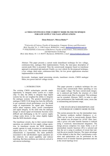
A <strong>CMOS</strong> <strong>CONTINUOUS</strong>-<strong>TIME</strong> <strong>CURRENT</strong> <strong>MODE</strong> <strong>FILTER</strong> TECHNIQUE<br />
FOR LOW SUPPLY VOLTAGE APPLICATIONS<br />
Elena Doicaru*, Mircea Bodea**<br />
*University of Craiova, Faculty of Automation, Computer Science and Electronics<br />
Blvd. Decebal, Nr. 5, 1100 Craiova, ROMANIA, e-mail: dmilena@electronics.ucv.ro<br />
** POLITEHNICA University of Bucharest, Faculty of Electronics, Telecommunication<br />
and Information Technology<br />
Blvd. Iuliu Maniu, Nr. 1-3, 061071 Bucharest, ROMANIA, e-mail: mircea.bodea@yahoo.com<br />
Abstract: This paper presents a current mode (translinear) technique for low voltage,<br />
continuous-time, analogue filter implementation. Firstly, the state-space description of<br />
current-mode filter is presented. Then the current-mode integrator based on translinear<br />
approach is presented and analyzed. Finally, as a test vehicle for the proposed technique,<br />
a low voltage, third order, continuous-time filter, for low power applications structure<br />
implementation is described.<br />
Keywords: Analogue signal processing circuits, translinear circuits, <strong>CMOS</strong> analogue<br />
filters, low power and low voltage circuits.<br />
1. INTRODUCTION<br />
The existing <strong>CMOS</strong> technologies provide ample<br />
opportunity to integrate entire system on a single<br />
chip. To date, the ability to integrate large digital<br />
systems has far out weighted the ability to integrate<br />
the analogue systems. The greatest impediment to<br />
analogue <strong>CMOS</strong> VLSI design has been the difficulty<br />
to get consistent circuit performance over the broad<br />
range of requirements for signal gain, frequency<br />
and/or phase response, delay, power consumption<br />
and signal integrity. In the same time the analogue<br />
design in mixed signal environments becomes more<br />
difficult and challenging as the IC’s power supply<br />
voltage scales down, to the values slightly higher<br />
than the MOS threshold voltage.<br />
The translinear circuits, due to their current domain<br />
operation, are suitable for low supply voltage operation.<br />
In translinear circuits the MOS transistors<br />
usually operate in weak inversion (or sub-threshold)<br />
region, (Enz et al., 1995), where the current-voltage<br />
characteristic is exponential. The main problems<br />
associated to the sub-threshold region operation are<br />
the relatively low speed capability and inferior<br />
matching. But these problems are relatively solved in<br />
sub-micron technology.<br />
This paper presents a synthesis technique for continuous<br />
time current-mode filters operating at very<br />
low supply voltage. The basic current-mode integrator<br />
is analyzed and finally the structure of a third<br />
order current-mode filter is presented. This technique<br />
can be extended, (Doicaru, 2007), in order to optimize<br />
performances like bandwidth, noise, errors due<br />
to mismatching and dynamic range.<br />
2. THE STATE-SPACE DESCRIPTION AND<br />
SYNTHESIS OF <strong>CURRENT</strong>-<strong>MODE</strong> <strong>FILTER</strong><br />
This section presents the way the intermediate transfer<br />
function synthesis method (Snelgrove et al.,<br />
1986) can be used in current-mode domain filters.<br />
The method was developed for AO-RC filter; basically<br />
a given n-th order transfer function is realized<br />
using n resistively interconnected integrators. The<br />
design process comprises two steps: firstly a set of<br />
intermediate transfer functions (IFs) is selected and<br />
then the set is using in synthesis of circuit that realized<br />
the given transfer function. The major advantage<br />
of this method is that the filter’s performance evaluation<br />
and optimization can be performed at the<br />
abstract level of transfer function generation and not<br />
at the circuit topology level.
The state-variable formulation of the AO-RC is<br />
s ⋅ x(s)<br />
= A ⋅ x(s)<br />
+ b ⋅ u(s)<br />
+ ε(s)<br />
y(s)<br />
= c<br />
T<br />
⋅ x(s)<br />
+ d ⋅ u(s)<br />
(1)<br />
where the vector x(s) represents the circuit state<br />
(integrators outputs), matrix A describes the interconnections<br />
between the n integrators, vector b contains<br />
the coefficients that multiply the input signal u(s) in<br />
order to be applied to the integrators inputs, vector c<br />
contains the coefficients required to form the output,<br />
scalar d is the coefficient of the feedthrough component<br />
from input to output, and ε(s) is the vector containing<br />
the noise component at the integrator inputs.<br />
The dual sets of IFs, {f i (s)} and {g i (s)} are given by:<br />
∆ xi<br />
( s)<br />
−1<br />
fi<br />
(s) = ; f(<br />
s) = (s ⋅ I − A ) ⋅ b<br />
u( s)<br />
∆ y( s) T T<br />
−1<br />
gi<br />
(s) = ; g (s) = c (s ⋅ I − A )<br />
εi<br />
( s)<br />
(2)<br />
The set {f i (s)} contains the transfer function from the<br />
filter input to the integrator outputs, and the set,<br />
{g i (s)}, can be physically interpreted as the integrators<br />
noise gains. Given a transfer function t(s), IF<br />
synthesis is based on choosing a set of linearly<br />
independent functions, {f i (s)}, having identical<br />
denominator polynomials, e(s), and arbitrary<br />
numerator polynomials of degree less than n. From<br />
this set the {A, b, c, d} parameters can be obtained<br />
using the following relation:<br />
−1<br />
T T −1<br />
A = F⋅E⋅<br />
F , b = F⋅1,<br />
c = t ⋅F<br />
,<br />
T<br />
d = tn+<br />
1, t(s)<br />
= t ⋅v(s)<br />
+ tn+<br />
1,<br />
f (s) = F⋅<br />
v(s)<br />
, g(s)<br />
= G ⋅v(s)<br />
,<br />
1<br />
v<br />
i<br />
(s) = , i = 1,<br />
n,<br />
s − ei<br />
T −1<br />
G = H⋅F<br />
(3)<br />
where t is a vector containing the t(s) n residues at<br />
the poles, t n+1 – the residue at s=∞, F – a matrix containing<br />
the residues of the f functions evaluated at the<br />
poles, G – a matrix of the residues of the g functions,<br />
e i – the e(s) roots, E – the diagonal matrix having the<br />
natural modes e i as its elements, H – a diagonal matrix<br />
formed from the residues of t(s), and<br />
1 = (1, 1, ...1) T .<br />
The sensitivities of filter directly depend of IFs set:<br />
t(s)<br />
Aij<br />
S = gi<br />
(s) ⋅ fi<br />
(s) ⋅ ,<br />
Aij<br />
t(s)<br />
t(s)<br />
b t(s)<br />
c<br />
S = g (s) i , S f (s) i<br />
i ⋅ = i ⋅<br />
bi<br />
t(s)<br />
ci<br />
t(s)<br />
t(s)<br />
d t(s)<br />
s<br />
Sd<br />
= , S = f (s) g (s) ,<br />
t(s)<br />
γi<br />
(s) i ⋅ i ⋅<br />
t(s)<br />
t(s)<br />
t(s)<br />
γi<br />
(s)<br />
S = S ⋅ S<br />
µ i (s) γi<br />
(s) µ i (s)<br />
(4)<br />
In the above equations γ i is the integrator gain and<br />
µ i (s) is the operational amplifier gain.<br />
Noise signals injected at integrator inputs can be<br />
modelled by ε(s). Assuming white input noise, with<br />
spectral density N<br />
is given by<br />
2<br />
i<br />
, the output noise power spectrum<br />
2<br />
2<br />
n0 )<br />
i<br />
P<br />
with a rms level of<br />
where<br />
( ω) = Ni<br />
⋅ ∑ gi<br />
( jω<br />
(5)<br />
2<br />
i<br />
P 0( ω) = N ∑ g ( jω)<br />
(6)<br />
n<br />
g ( jω)<br />
i<br />
i<br />
2<br />
= ∫<br />
∞ 2<br />
i −∞<br />
g ( jω) dω<br />
2 i<br />
(7)<br />
This description can be adapted to the current-mode<br />
filter. The current through the k-th capacitor of the<br />
current-mode filter is<br />
Ck<br />
v&<br />
Ck = iCk1<br />
+ iC k 2 + ... + iC k n + iCbk<br />
=<br />
* * * * *<br />
= a k 1i1<br />
+ a k 2i2<br />
+ ... + a kn v n + b k i in + ε k<br />
2<br />
2<br />
(8)<br />
where i Ckj , k, j=1÷n, is the k-th capacitor current component<br />
dependent on output current i j , j=1÷n, i j is the<br />
j-th current-mode integrator output current, i in is the<br />
filter input current,<br />
*<br />
a kj , k, j=1÷n and<br />
*<br />
b k , k=1÷n,<br />
coefficients describes the capacitor current components<br />
dependence on the output currents of the<br />
current-mode integrators, respectively, on the filter<br />
* *<br />
input current, and ε k = ∑ j ε kj is the total noise<br />
current through capacitor.<br />
Using convenient circuit technique to implement a<br />
logarithmic dependence between capacitor voltage,<br />
v Ck , and output current of current-mode integrator, i k ,<br />
v = V ln ( i / I )<br />
(9)<br />
Ck<br />
x<br />
where V x and I y are scale factors, the capacitor voltage<br />
derivative, v& Ck , becomes:<br />
d<br />
k<br />
y<br />
Vx<br />
i<br />
v& k<br />
Ck = .<br />
(10)<br />
ik<br />
dt<br />
Using the translinear loops one get for each component<br />
of the capacitor current<br />
*<br />
*<br />
i Ckj ik<br />
= akj<br />
i j , iCbk<br />
ik<br />
= bk<br />
iin<br />
(11)<br />
and equation (8) becomes<br />
d<br />
d<br />
ik<br />
t<br />
where<br />
akn<br />
=<br />
1 2 2<br />
*<br />
kn<br />
ak1i<br />
+ ak<br />
i<br />
+ ... +<br />
*<br />
b k<br />
aknv<br />
+<br />
bk<br />
n<br />
i in<br />
+ ε<br />
k<br />
(12)<br />
= a /( C V ), b = /( C V ), ε = ε /( C V ) (13)<br />
k<br />
x<br />
k<br />
The circuit resulted by interconnection of n current<br />
mode integrators with translinear loops can be<br />
described by the same state-variable formulation (1):<br />
k<br />
x<br />
k<br />
*<br />
k<br />
s ⋅ x(s)<br />
= A ⋅ x(s)<br />
+ b ⋅iin(s)<br />
+ ε(s)<br />
T<br />
iout<br />
(s) = c ⋅ x(s)<br />
+ d ⋅iin(s)<br />
k<br />
x<br />
(14)<br />
where the states x k are represented by the integrators<br />
output current, matrix element A kj is implemented by<br />
a translinear loop with input current x k and output the<br />
component i Ckj of the current through k-th, the vector
element b k is implemented by translinear loop from<br />
the input i in to state k, c k is multiplication coefficient<br />
of state k required to form the output current of the<br />
filter i out , d is multiplication coefficient of input current<br />
i in and ε (s)<br />
can model the current noise at the<br />
input of the k-th current integrator.<br />
1<br />
I D /I F<br />
5%<br />
saturation<br />
G<br />
D<br />
I R<br />
B<br />
I F<br />
S<br />
So the meaning of {f k (s)} IF's set is the same as in the<br />
OA-RC filter synthesis (the state k and the input<br />
signal ratio) and the physical meaning of {g k (s)} IF's<br />
set is the noise gain to the input of integrator k at<br />
output of filter. We can conclude that the all results<br />
obtained in the OA-RC filter synthesis can be applied<br />
to the current-mode filter synthesis.<br />
3. MOS TRANSISTOR <strong>CURRENT</strong>-VOLTAGE<br />
CHARACTERISTICS<br />
This section presents a brief review of the MOS transistor<br />
I-V characteristics, focused on weak inversion<br />
operation.<br />
The MOS transistor drain current equation valid in<br />
all operating regions is (Enz et al., 1995):<br />
with<br />
I<br />
D<br />
VD<br />
∫<br />
= β ( −Q<br />
/ C ) dV<br />
(15)<br />
VS<br />
i<br />
ox<br />
β = µC ox ( W / L)<br />
(16)<br />
where W and L are the channel width and length,<br />
C ox – gate capacitance per unit area, µ – charge<br />
carrier mobility, Q i – induced mobile charge in<br />
channel, V D , V S – drain, source voltages referred to<br />
the local substrate, V – channel potential. Equation<br />
(15) may be decomposed, (Vittoz, 1994), into:<br />
I<br />
D<br />
∞<br />
= β ∫<br />
( −Qi<br />
/ Cox<br />
)dV<br />
− β∫<br />
∞<br />
VS V D<br />
= IF − I R<br />
( −Q<br />
/ C<br />
i<br />
ox<br />
) dV<br />
(17)<br />
where I F is called forward current (controlled by<br />
source voltage V S ) and I R is called reverse current<br />
(controlled by drain voltage V D ). Taking into account<br />
weak inversion channel charge dependency on<br />
channel potential<br />
I F and I R are given by<br />
( VP − V ) / V<br />
Q<br />
T<br />
i / Cox<br />
~ e<br />
(18)<br />
I F ~ β e<br />
( R)<br />
( V −V<br />
P<br />
S(<br />
D)<br />
) / V<br />
And the drain current equation results:<br />
V<br />
ID<br />
= IS<br />
e<br />
P<br />
/ V<br />
T<br />
⎡ −V<br />
⎢e<br />
⎣<br />
S<br />
/ V<br />
T<br />
T<br />
−V<br />
− e<br />
D<br />
/ V<br />
In terms of V GS and V GD equation (20) becomes<br />
( V<br />
ID<br />
= IS<br />
e<br />
V ) / V<br />
P − G<br />
T<br />
⎡ −V<br />
⎢e<br />
⎣<br />
GS<br />
/ V<br />
T<br />
−V<br />
− e<br />
T<br />
GD<br />
⎤<br />
⎥<br />
⎦<br />
/ V<br />
T<br />
⎤<br />
⎥<br />
⎦<br />
(19)<br />
(20)<br />
(21)<br />
where I S is a specific current (limit of weak<br />
inversion), proportional to W/L<br />
0<br />
0 1 2 3 4 5 6 V G<br />
DS /V T<br />
I R<br />
V S =const.<br />
S<br />
(a)<br />
(b)<br />
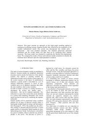
Fig. 1. (a) The operation regions in weak inversion of<br />
the MOS transistor; (b) Non-saturated MOS transistor<br />
is equivalent to two saturated transistors<br />
anti-parallel connected.<br />
I<br />
S<br />
e<br />
( VP<br />
−VG<br />
) / VT<br />
=<br />
W<br />
L<br />
I<br />
◊<br />
( V )<br />
G<br />
(22)<br />
I ◊ ( V G ) is the square transistor zero-bias ( V GS = 0 )<br />
current.<br />
Using (22) I F and I R equations become:<br />
I<br />
I<br />
non-saturation<br />
F<br />
R<br />
W<br />
= ⋅ I<br />
L<br />
W<br />
= ⋅ I<br />
L<br />
◊<br />
◊<br />
( V )<br />
G<br />
( V )<br />
G<br />
⋅ e<br />
⋅ e<br />
V<br />
V<br />
GS<br />
GD<br />
/ V<br />
T<br />
/ V<br />
T<br />
(23)<br />
If I R
(a)<br />
(b)<br />
Fig. 2. The current mode integrator with translinear loop for capacitor current component I Cij .<br />
(a) Circuit schematic; (b) Circuit symbolic representation.<br />
Therefore, using the decomposition technique<br />
described above (see Fig. 2.b.), the fictitious<br />
transistors M 2* , M 4* , M 6* and M 13* (dashed line in<br />
Fig. 2.b) were added in order to account the nonsaturated<br />
operation of these transistors. This way all<br />
transistors can now be regarded as saturated, I R
But<br />
and<br />
I<br />
I<br />
I<br />
I<br />
D4*<br />
D6*<br />
D2*<br />
D13*<br />
I0<br />
+ I<br />
I<br />
0<br />
( iin<br />
+ I IN ) I0<br />
=<br />
I<br />
0<br />
+ I<br />
( iout<br />
+ IOUT<br />
) I<br />
=<br />
I0<br />
+ I<br />
( I0<br />
+ I ) I0<br />
=<br />
iout<br />
+ IOUT<br />
I I IN<br />
=<br />
i + I<br />
I<br />
out<br />
D10<br />
= I<br />
OUT<br />
D9<br />
0<br />
0<br />
i out + I<br />
I<br />
0<br />
OUT<br />
I D10<br />
= I D4<br />
− I D4*<br />
− I D5<br />
+ I D6<br />
− I<br />
( iin<br />
+ I IN ) I0<br />
= iin<br />
+ I IN −<br />
− I0<br />
+<br />
I0<br />
+ I<br />
( iout<br />
+ IOUT<br />
) I0<br />
i out + IOUT<br />
−<br />
=<br />
I0<br />
+ I<br />
( iin<br />
+ I IN ) I ( iout<br />
+ IOUT<br />
) I<br />
=<br />
+<br />
− I<br />
I + I I + I<br />
=<br />
i<br />
out<br />
0<br />
= ( I − I<br />
IN<br />
I I<br />
+ I<br />
IN<br />
) − ( I −<br />
i<br />
OUT<br />
out<br />
I I<br />
+ I<br />
IN<br />
OUT<br />
− I<br />
D6*<br />
I D9<br />
= iC<br />
+ I x − I0<br />
+ I D2<br />
− I D2*<br />
=<br />
( I0<br />
+ I ) I0<br />
= iC<br />
+ I x − I0<br />
+ I + I0<br />
−<br />
iout<br />
+ IOUT<br />
( I0<br />
+ I ) I0<br />
= iC<br />
+ I<br />
x<br />
+ I −<br />
iout<br />
+ IOUT<br />
I<br />
x<br />
= ( I − I IN ) − ( I D13<br />
− I D13*<br />
− I<br />
IN<br />
0<br />
D16<br />
=<br />
) =<br />
=<br />
) =<br />
(33)<br />
(34)<br />
(35)<br />
Substituting equations (33) and (34) into general<br />
translinear loop equations (32) yields:<br />
( i in + I IN ) I = ( iC<br />
+ I x ) ( iout<br />
+ IOUT<br />
)<br />
( i + I ) I = i ( i + I ) + I I<br />
in<br />
IN<br />
in<br />
C<br />
out<br />
i I = i +<br />
OUT<br />
C ( iout<br />
IOUT<br />
)<br />
IN<br />
(36)<br />
Noting that the capacitor voltage, v C , is the difference<br />
between the gate-source voltages of M 7 and M 8<br />
v<br />
C<br />
i i I<br />
v<br />
out + OUT<br />
= (37)<br />
I<br />
D7<br />
GS7 − vGS8<br />
= VT<br />
ln = VT<br />
ln<br />
I0<br />
and replacing (37) into the capacitor current equation<br />
dvC<br />
iC<br />
= C<br />
(38)<br />
dt<br />
and taking into account the lower equation (36)<br />
results the capacitor current<br />
i<br />
C<br />
C VT<br />
diout<br />
= (39)<br />
iout<br />
+ IOUT<br />
dt<br />
Finally we get a linear integrator function:<br />
0<br />
Fig. 3. The third order filter structure.<br />
I<br />
iout = ∫iin<br />
d t<br />
(40)<br />
CV<br />
T<br />
The integrator operates correctly as long as the<br />
quiescent values of the currents I, I 0 , I IN , I OUT is<br />
chosen so that the integrator’s transistors drain<br />
currents to be strictly positive for the input voltage<br />
range, (Seevinck, 1988).<br />
5. THE THIRD ORDER<br />
<strong>CURRENT</strong> <strong>MODE</strong> <strong>FILTER</strong><br />
As an example of the application of the synthesis<br />
technique presented in Section 2 a third order current<br />
mode filter have been synthesised. The transfer<br />
function of the filter is:<br />
1<br />
t (s) =<br />
3 2<br />
(41)<br />
s + 2s + 2s + 1<br />
The system parameters {A,b,c,d} resulted using the<br />
SSAF program (Doicaru et. al., 2007) for orthonormal<br />
IFs are:<br />
⎡ 0<br />
⎢<br />
A =<br />
⎢<br />
0<br />
⎢<br />
⎣−<br />
0,707<br />
⎡ 0 ⎤<br />
⎢ ⎥<br />
b =<br />
⎢<br />
0<br />
⎥<br />
⎢<br />
⎣0,798<br />
⎥<br />
⎦<br />
0,707 0 ⎤<br />
⎥<br />
−1,225<br />
− 2<br />
⎥<br />
0 1,225⎥<br />
⎦<br />
⎡ 0 ⎤<br />
⎢ ⎥<br />
c =<br />
⎢<br />
0<br />
⎥<br />
⎢<br />
⎣1,447⎥<br />
⎦<br />
d = 0<br />
(42)<br />
We choose this type of IFs to be generated by SSAF<br />
because the structures to be synthesised using orthonormal<br />
intermediate transfer functions generally have<br />
good dynamic range, good signal swing and low sensitivity.<br />
The structure of the current mode filter characterised<br />
by parameters (42) is presented in Fig. 3 and the<br />
system equation are:<br />
i<br />
i<br />
i<br />
i<br />
C1<br />
C2<br />
C3<br />
out<br />
= iC12<br />
= iC<br />
22 + i<br />
= iC<br />
31 + i<br />
= c i<br />
3 out3<br />
C23<br />
C33<br />
+ i<br />
Cb3<br />
(43)
Using the relations developed in Section 3 the system<br />
(43) becomes:<br />
out3<br />
C1V<br />
T diout1<br />
iout2<br />
I<br />
= 12<br />
iout1<br />
+ IOUT1<br />
dt<br />
iout1<br />
+ IOUT1<br />
C3VT<br />
iout3<br />
+ I<br />
iout1I<br />
−<br />
i + I<br />
C2VT<br />
diout2<br />
=<br />
iout2<br />
+ IOUT<br />
2 d t<br />
iout2<br />
I22<br />
iout3<br />
I<br />
= −<br />
− 23<br />
iout2<br />
+ IOUT<br />
2 iout2<br />
+ IOUT<br />
2<br />
OUT 3<br />
31<br />
OUT 3<br />
di<br />
dt<br />
out3<br />
+<br />
i<br />
=<br />
iout3<br />
I<br />
+ I<br />
out3<br />
i = c i<br />
out<br />
33<br />
OUT 3<br />
3 out3<br />
+<br />
i<br />
out3<br />
i I<br />
+ I<br />
in b3<br />
OUT 3<br />
and the state-space description of this filter is:<br />
di<br />
d t<br />
di<br />
dt<br />
out3<br />
out2<br />
= −<br />
It is obvious that:<br />
diout1<br />
iout<br />
I<br />
= 2 12<br />
d t C1VT<br />
== −<br />
iout1I<br />
C V<br />
3<br />
iout2<br />
I<br />
C V<br />
31<br />
T<br />
2<br />
22<br />
T<br />
iout3<br />
I<br />
+<br />
C V<br />
iout3<br />
I<br />
−<br />
C V<br />
3<br />
i out = c3iout3<br />
33<br />
T<br />
2<br />
23<br />
T<br />
i I<br />
+<br />
C V<br />
in b3<br />
I12<br />
a12<br />
= ;<br />
C1VT<br />
I 22<br />
I23<br />
a22<br />
= , a23<br />
= ;<br />
C2VT<br />
C2VT<br />
I31<br />
I33<br />
a31<br />
= , a33<br />
= ;<br />
C3VT<br />
C3VT<br />
Ib3<br />
b3<br />
= ;<br />
C3VT<br />
( W / L)<br />
outMOS<br />
c3<br />
=<br />
.<br />
( W / L)<br />
TLb3<br />
3<br />
T<br />
(44)<br />
(45)<br />
(46)<br />
In the future work the current-mode filters synthesis<br />
method presented in this paper will be refined being<br />
focused on optimization of specific performances<br />
like bandwidth, noise, errors du mismatching and<br />
dynamic range.<br />
6. CONCLUSIONS<br />
Future analogue circuits will have to operate successfully<br />
at supply voltages slightly higher than the MOS<br />
transistor threshold voltage. So, the suitable topologies<br />
for signal processing at such low values of<br />
supply voltages are the translinear circuits because<br />
are operating in current domain and in this way the<br />
very small voltage swings are avoided.<br />
This paper presented a technique for very low supply<br />
voltage, continuous time, current-mode filters synthesis<br />
based on the intermediate transfer functions<br />
method. This method has the distinct advantage of<br />
filter performance optimization at the abstract level<br />
of IFs, not at the topological level. In paper is also<br />
presented the basic cell of the filter – the current<br />
mode integrator, suitable for static and dynamic<br />
analogue signal processing and very low supply<br />
voltage operation. The minimum value of supply<br />
voltage required for this circuit is given by the sum<br />
of the MOS transistor threshold voltage and the<br />
drain-source saturation voltage.<br />
All transistors of these networks operate in weak<br />
inversion due to the requirements of translinear<br />
principle to have an exponential I-V characteristic<br />
and the very low power supply voltage. Therefore,<br />
bandwidth will be limited and the circuits will be<br />
sensitive to the threshold voltage matching. Finally,<br />
as a test vehicle for the proposed synthesis method,<br />
the structure of a third order continuous-time filter<br />
for low power applications was is presented and<br />
analyzed.<br />
ACKNOWLEDGMENT<br />
This work was supported by the CNCSIS Research<br />
Project no. 29C/08.05.2007, theme no. 5, CNCSIS<br />
code no.602.<br />
REFERENCES<br />
Doicaru E., L. Barbulescu, C. Dan, (2007). SSAF –<br />
A Powerful Tool for High-Order Analogue<br />
Continuous Time Filter Synthesis, WSEAS<br />
European Computing Conference, Athens,<br />
Greece, September 25-27, 2007, accepted.<br />
Doicaru, E., M. Bodea, C. Dan, Current-mode filters<br />
advanced synthesis methods, based on intermediate<br />
transfer function algorithm, unpublished<br />
works.<br />
Enz, C.C., F. Krummenacher and E. Vittoz (1995).<br />
An analytical MOS transistor model valid in all<br />
regions of operation and dedicated to low-voltage<br />
and low-current applications. IEEE Journal<br />
of Analog Integrated Circuits Signal Processing,<br />
8, 83-114.<br />
Seevinck, E., (1988). Synthesis of TL Networks,<br />
Analysis and Synthesis of Translinear Integrated<br />
Circuits, Elsevier, page 69-132, Amsterdam.<br />
Snelgrove W.M. and A.S. Sedra (1986). Synthesis<br />
and Analysis of State-Space Active Filters Using<br />
Intermediate Transfer Functions, IEEE Trans.<br />
Circuits and Systems, CAS-33, 287-300.<br />
Vittoz, E. (1994). Micropower techniques, Design of<br />
VLSI Circuits for Telecommunication and Signal<br />
Processing, Prentice Hall.<br />
Vittoz, E., and J Fellrath (1997). <strong>CMOS</strong> analog integrated<br />
circuits based on weak inversion operation,<br />
IEEE J. Solid-State Circuits, 12, 224-231.