Dynamics and geometry optimization with ChemShell
Dynamics and geometry optimization with ChemShell
Dynamics and geometry optimization with ChemShell

You also want an ePaper? Increase the reach of your titles
YUMPU automatically turns print PDFs into web optimized ePapers that Google loves.
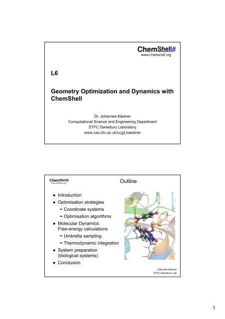
L6<br />
Geometry Optimization <strong>and</strong> <strong>Dynamics</strong> <strong>with</strong><br />
<strong>ChemShell</strong><br />
Dr. Johannes Kästner<br />
Computational Science <strong>and</strong> Engineering Department<br />
STFC Daresbury Laboratory<br />
www.cse.clrc.ac.uk/ccg/j.kaestner<br />
Outline<br />
● Introduction<br />
● Optimisation strategies<br />
− Coordinate systems<br />
− Optimisation algorithms<br />
● Molecular <strong>Dynamics</strong>:<br />
Free-energy calculations<br />
− Umbrella sampling<br />
− Thermodynamic integration<br />
● System preparation<br />
(biological systems)<br />
● Conclusion<br />
Johannes Kästner<br />
STFC Daresbury Lab<br />
1
<strong>ChemShell</strong><br />
GAUSSIAN<br />
TURBOMOLE<br />
GAMESS-UK<br />
MOLPRO<br />
MNDO<br />
NWCHEM<br />
<strong>ChemShell</strong><br />
Tcl scripts<br />
Integrated<br />
routines:<br />
data<br />
management<br />
<strong>geometry</strong><br />
<strong>optimization</strong><br />
molecular<br />
dynamics<br />
CHARMM<br />
academic<br />
CHARMm<br />
MSI<br />
GROMOS96<br />
DL_POLY<br />
GULP<br />
QM<br />
codes<br />
generic<br />
force fields<br />
QM/MM<br />
coupling<br />
MM<br />
codes<br />
Johannes Kästner<br />
STFC Daresbury Lab<br />
Why Optimisation<br />
● Find minima on the potential<br />
energy surface<br />
● Structure: equilibrium structure<br />
at stationary points (reactants or<br />
products)<br />
● Energy differences: ∆E ≈ ∆U<br />
● Saddle points: transition states<br />
− Activation energies<br />
− Reaction rates<br />
● All optimisation results: T=0<br />
Optimisation – Potential Energy<br />
Johannes Kästner<br />
STFC Daresbury Lab<br />
2
Free-energy differences:<br />
● Umbrella sampling<br />
● Thermodynamic integration<br />
Finite-temperature effects<br />
Why <strong>Dynamics</strong><br />
To establish a minimum as<br />
being “relatively global”<br />
Global averages<br />
Molecular <strong>Dynamics</strong> – Free Energy<br />
Johannes Kästner<br />
STFC Daresbury Lab<br />
Free Energy<br />
● Driving force of chemical reaction<br />
● Helmholtz energy A = U – TS at<br />
constant volume<br />
∆ ‡ A<br />
● Gibbs energy G = H – TS at<br />
constant pressure<br />
● ∆ r A defines the equilibrium constant:<br />
∆ r A = – RT ln K<br />
● ∆ ‡ A determines the reaction rate<br />
Reactant<br />
Transition state<br />
Product<br />
∆ r A<br />
Johannes Kästner<br />
STFC Daresbury Lab<br />
3
Optimisation in <strong>ChemShell</strong><br />
Established St<strong>and</strong>ards<br />
● Z-matrix optimisation <strong>with</strong> a quasi-Newton optimiser<br />
(st<strong>and</strong>ard in quantum chemistry)<br />
● Cartesian coordinates <strong>with</strong> a conjugate gradient<br />
optimiser (st<strong>and</strong>ard in MD)<br />
Johannes Kästner<br />
STFC Daresbury Lab<br />
4
Coordinate Systems<br />
● Cartesian coordinates:<br />
− O(N 0 )<br />
− Highly coupled (torsions)<br />
● Z-Matrix:<br />
− O(N)<br />
− Less coupled<br />
− Biased (different ways to set up a Z-matrix)<br />
● Redundant internal coordinates<br />
− O(N 3 )<br />
− Less coupled<br />
− Nowadays st<strong>and</strong>ard for small systems<br />
Johannes Kästner<br />
STFC Daresbury Lab<br />
HDLC coordinates<br />
● Hybrid DeLocalised internal Coordinates<br />
● Divide <strong>and</strong> conquer: large molecule is split<br />
into fragments<br />
● Internal coordinates <strong>with</strong>in each fragment<br />
● Coupling of the fragments via Cartesian<br />
coordinates<br />
● O(N)<br />
● Less coupled<br />
● Available in <strong>ChemShell</strong> in HDLCopt<br />
Billeter, Turner, Thiel Phys. Chem. Chem. Phys. 2, 2177 (2000)<br />
Johannes Kästner<br />
STFC Daresbury Lab<br />
5
Optimisation Algorithms<br />
● Determination of the search direction<br />
● First-order methods: gradient<br />
− Steepest descent<br />
− Conjugate gradient<br />
− Damped dynamics<br />
● Second order methods: gradient <strong>and</strong> Hessian<br />
− Quasi-Newton methods<br />
− RFO<br />
− BFGS (accumulated Hessian)<br />
− L-BFGS (accumulated Hessian, O(N))<br />
Johannes Kästner<br />
STFC Daresbury Lab<br />
Transition-State Search Algorithms<br />
● First order saddle points:<br />
− Zero gradient<br />
− One negative eigenvalue of the Hessian,<br />
all others positive<br />
● P-RFO (requires accurate Hessian)<br />
● Dimer method (no Hessian required)<br />
● Newton-Raphson (finds any extremum)<br />
Johannes Kästner<br />
STFC Daresbury Lab<br />
6
Optimisers in <strong>ChemShell</strong><br />
Four optimisers available:<br />
● Newopt: flexible optimizer.<br />
Methods: BFGS, (P)RFO, DIIS,<br />
conjugate gradient, steepest descent, …<br />
Coordinate systems: Cartesian or z-matrix<br />
● HDLCopt: fastest for large systems, O(N)<br />
Methods: L-BFGS, P-RFO (for transition state search)<br />
Coordinate systems: hybrid delocalized internal coordinates<br />
● dimer: TS search <strong>with</strong> the dimer method<br />
● opt<br />
Johannes Kästner<br />
STFC Daresbury Lab<br />
Johannes Kästner<br />
STFC Daresbury Lab<br />
7
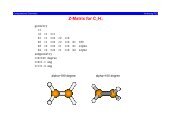
Small Molecules: newopt – zopt<br />
Optimisation of a molecule given as z-matrix using the<br />
BFGS method:<br />
newopt \<br />
function= zopt : { \<br />
zmatrix= water.zz4 \<br />
theory= mndo } \<br />
method= bfgs<br />
Johannes Kästner<br />
STFC Daresbury Lab<br />
Large Molecules: HDLCopt<br />
● Small molecule, redundant internals:<br />
hdlcopt coords=c \<br />
residues= [ res_selectall coords=c ] \<br />
theory= mndo<br />
● Large molecule, provided as pdb file, HDLCs:<br />
set residues [ pdb_to_res 1PBE.pdb ]<br />
hdlcopt coords=c \<br />
residues= $residues \<br />
constraints= {{bond 3 5} {angle 3 5 6}} \<br />
theory= mndo<br />
Johannes Kästner<br />
STFC Daresbury Lab<br />
8
Dimer Method for TS search<br />
● Dimer: two images of the system,<br />
constant distance<br />
● Rotation: difference of the forces<br />
● Movement:<br />
− In dimer direction: against the force<br />
− Perpendicular to dimer direction:<br />
along the force<br />
● Converges to first-order saddle points<br />
● No Hessian required: for large systems<br />
Johannes Kästner<br />
STFC Daresbury Lab<br />
Dimer method in <strong>ChemShell</strong><br />
dimer coords=c mode=3 \<br />
maxcyc=100 \<br />
theory= gamess : $gamess_args<br />
Johannes Kästner<br />
STFC Daresbury Lab<br />
9
Outlook: Nudged Elastic B<strong>and</strong><br />
● Multiple images, connected by “springs”<br />
● Converges to the minimum-energy path<br />
● Climbing image: transition state<br />
● Evolved, but can cover difficult reactions<br />
● Implementation in <strong>ChemShell</strong> is in “beta stage”<br />
Johannes Kästner<br />
STFC Daresbury Lab<br />
Exploiting QM/MM capabilities:<br />
Micro-iterative QM/MM optimisation<br />
One QM step<br />
Complete MM<br />
optimisation<br />
● Electrostatic embedding: ESP charges<br />
calculated on the fly<br />
● Optimisation effort becomes independent of<br />
the system size<br />
● Saves a factor of 2–10 in CPU time<br />
● hdlcopt<br />
inner_atoms= { 1 2 14 15 } mcore=true<br />
Kästner, S. Thiel, Senn, Sherwood, W. Thiel,<br />
J. Chem. Theory Comput. online (2007)<br />
Johannes Kästner<br />
STFC Daresbury Lab<br />
10
Molecular <strong>Dynamics</strong> in <strong>ChemShell</strong><br />
NVE, NVT, NPT,<br />
constant friction<br />
MD driver<br />
from DL_POLY<br />
Rigid body motion<br />
(quaternions)<br />
Monte Carlo<br />
sampling<br />
Distance <strong>and</strong><br />
other constraints<br />
(SHAKE)<br />
Johannes Kästner<br />
STFC Daresbury Lab<br />
11
Free-Energy Methods I<br />
● Fixed constraint<br />
− Thermodynamic integration: sampling the mean force<br />
● Continuously changing constraint<br />
− Slow growth: sampling the mean force<br />
− Fast growth: fast changing constraint, exponential<br />
average of the energy change<br />
● Free-energy perturbation: instantaneous changes,<br />
exponential average of the energy change<br />
Johannes Kästner<br />
STFC Daresbury Lab<br />
Free-Energy Methods II<br />
● Fixed restraint (bias)<br />
− Umbrella sampling: sampling the distribution of the<br />
reaction coordinate<br />
● Continuously changing restraint<br />
− Steered molecular dynamics<br />
● Hessian: quadratic approximation, anharmonicities<br />
neglected<br />
● …<br />
Johannes Kästner<br />
STFC Daresbury Lab<br />
12
Umbrella Sampling<br />
● A number of windows, each <strong>with</strong> a<br />
restraint (bias) centred at different<br />
points along the reaction coordinate<br />
● Distribution along the reaction<br />
coordinate is sampled<br />
● Analysis by<br />
− WHAM or<br />
− Umbrella Integration<br />
provides the free-energy difference<br />
● Restraints available in <strong>ChemShell</strong>:<br />
bond, angle, torsion, difference between 2, 3, <strong>and</strong> 4<br />
bond lengths<br />
● Use the NHC thermostat: nosehoover=4<br />
biased potential<br />
potential energy surface<br />
Johannes Kästner<br />
STFC Daresbury Lab<br />
Thermodynamic Integration<br />
● A number of windows, each<br />
constrained to a particular value<br />
of the reaction coordinate<br />
● Shake-like constraint (Lagrange<br />
multiplier)<br />
● Force on the constraint is averaged<br />
● Integration of these mean forces<br />
provides an approximate free-energy<br />
change<br />
● Metric tensor corrections<br />
● Constraints available in <strong>ChemShell</strong>:<br />
bond, torsion, difference between 2<br />
bond lengths<br />
constrained to this value<br />
potential energy surface<br />
Johannes Kästner<br />
STFC Daresbury Lab<br />
13
Exploiting QM/MM functionality:<br />
QM/MM-FEP<br />
Reaction profile:<br />
● Full QM/MM<br />
calculations<br />
● QM <strong>and</strong> MM atoms<br />
optimized<br />
Sampling:<br />
● Frozen QM part<br />
● MM-dynamics<br />
∆A = ∆E<br />
+ ∆A<br />
qm<br />
qm/mm<br />
Zhang, Liu, Yang J. Chem. Phys. 112, 3483 (2000)<br />
Johannes Kästner<br />
STFC Daresbury Lab<br />
System Preparation<br />
14
Setup of QM/MM calculations of proteins<br />
Starting point: pdb file<br />
Check errors: What If<br />
Add hydrogen<br />
Pronation state (PropKa)<br />
Solvate the protein in water<br />
Equilibrate solvate<br />
Equilibrate the whole (MM) system<br />
Structure optimisation at the QM/MM level<br />
Johannes Kästner<br />
STFC Daresbury Lab<br />
Fluorinase: Setup<br />
QM/MM setup:<br />
● Solvated in a 25 Å water sphere<br />
● QM method: DFT (BP86) <strong>with</strong><br />
Turbomole<br />
● MM method: CHARMM force<br />
field <strong>with</strong> DL_POLY in<br />
<strong>ChemShell</strong><br />
● Electrostatic embedding<br />
(charge shift)<br />
● HDLCopt, shell of 8 Å around<br />
the active site optimized<br />
Senn, O’Hagan, Thiel J. Am. Chem. Soc. 127, 13643 (2005)<br />
Johannes Kästner<br />
STFC Daresbury Lab<br />
15
Conclusions<br />
Optimisation:<br />
● Small molecules: newopt – zopt<br />
● Large systems: HDLCopt (possibly micro-iterative)<br />
Free-energy sampling:<br />
● Umbrella sampling (NHC thermostat)<br />
Further information:<br />
www.chemshell.org/manual<br />
www.chemshell.org/tutorial<br />
Johannes Kästner<br />
STFC Daresbury Lab<br />
16