Dynamics and geometry optimization with ChemShell
Dynamics and geometry optimization with ChemShell
Dynamics and geometry optimization with ChemShell

Create successful ePaper yourself
Turn your PDF publications into a flip-book with our unique Google optimized e-Paper software.
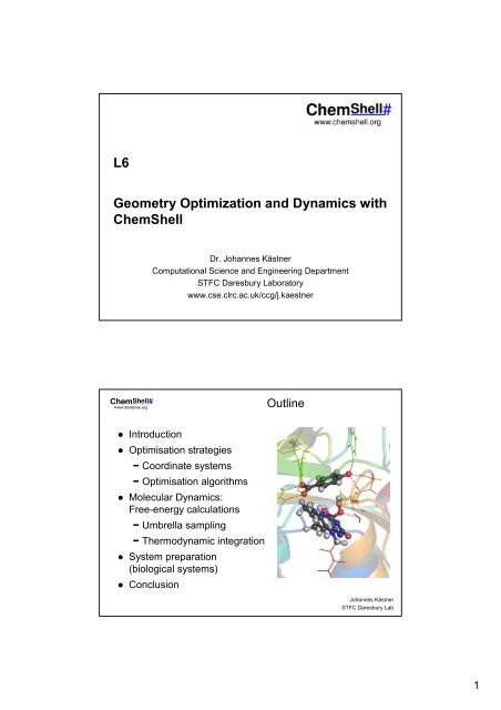
L6<br />
Geometry Optimization <strong>and</strong> <strong>Dynamics</strong> <strong>with</strong><br />
<strong>ChemShell</strong><br />
Dr. Johannes Kästner<br />
Computational Science <strong>and</strong> Engineering Department<br />
STFC Daresbury Laboratory<br />
www.cse.clrc.ac.uk/ccg/j.kaestner<br />
Outline<br />
● Introduction<br />
● Optimisation strategies<br />
− Coordinate systems<br />
− Optimisation algorithms<br />
● Molecular <strong>Dynamics</strong>:<br />
Free-energy calculations<br />
− Umbrella sampling<br />
− Thermodynamic integration<br />
● System preparation<br />
(biological systems)<br />
● Conclusion<br />
Johannes Kästner<br />
STFC Daresbury Lab<br />
1
<strong>ChemShell</strong><br />
GAUSSIAN<br />
TURBOMOLE<br />
GAMESS-UK<br />
MOLPRO<br />
MNDO<br />
NWCHEM<br />
<strong>ChemShell</strong><br />
Tcl scripts<br />
Integrated<br />
routines:<br />
data<br />
management<br />
<strong>geometry</strong><br />
<strong>optimization</strong><br />
molecular<br />
dynamics<br />
CHARMM<br />
academic<br />
CHARMm<br />
MSI<br />
GROMOS96<br />
DL_POLY<br />
GULP<br />
QM<br />
codes<br />
generic<br />
force fields<br />
QM/MM<br />
coupling<br />
MM<br />
codes<br />
Johannes Kästner<br />
STFC Daresbury Lab<br />
Why Optimisation<br />
● Find minima on the potential<br />
energy surface<br />
● Structure: equilibrium structure<br />
at stationary points (reactants or<br />
products)<br />
● Energy differences: ∆E ≈ ∆U<br />
● Saddle points: transition states<br />
− Activation energies<br />
− Reaction rates<br />
● All optimisation results: T=0<br />
Optimisation – Potential Energy<br />
Johannes Kästner<br />
STFC Daresbury Lab<br />
2
Free-energy differences:<br />
● Umbrella sampling<br />
● Thermodynamic integration<br />
Finite-temperature effects<br />
Why <strong>Dynamics</strong><br />
To establish a minimum as<br />
being “relatively global”<br />
Global averages<br />
Molecular <strong>Dynamics</strong> – Free Energy<br />
Johannes Kästner<br />
STFC Daresbury Lab<br />
Free Energy<br />
● Driving force of chemical reaction<br />
● Helmholtz energy A = U – TS at<br />
constant volume<br />
∆ ‡ A<br />
● Gibbs energy G = H – TS at<br />
constant pressure<br />
● ∆ r A defines the equilibrium constant:<br />
∆ r A = – RT ln K<br />
● ∆ ‡ A determines the reaction rate<br />
Reactant<br />
Transition state<br />
Product<br />
∆ r A<br />
Johannes Kästner<br />
STFC Daresbury Lab<br />
3
Optimisation in <strong>ChemShell</strong><br />
Established St<strong>and</strong>ards<br />
● Z-matrix optimisation <strong>with</strong> a quasi-Newton optimiser<br />
(st<strong>and</strong>ard in quantum chemistry)<br />
● Cartesian coordinates <strong>with</strong> a conjugate gradient<br />
optimiser (st<strong>and</strong>ard in MD)<br />
Johannes Kästner<br />
STFC Daresbury Lab<br />
4
Coordinate Systems<br />
● Cartesian coordinates:<br />
− O(N 0 )<br />
− Highly coupled (torsions)<br />
● Z-Matrix:<br />
− O(N)<br />
− Less coupled<br />
− Biased (different ways to set up a Z-matrix)<br />
● Redundant internal coordinates<br />
− O(N 3 )<br />
− Less coupled<br />
− Nowadays st<strong>and</strong>ard for small systems<br />
Johannes Kästner<br />
STFC Daresbury Lab<br />
HDLC coordinates<br />
● Hybrid DeLocalised internal Coordinates<br />
● Divide <strong>and</strong> conquer: large molecule is split<br />
into fragments<br />
● Internal coordinates <strong>with</strong>in each fragment<br />
● Coupling of the fragments via Cartesian<br />
coordinates<br />
● O(N)<br />
● Less coupled<br />
● Available in <strong>ChemShell</strong> in HDLCopt<br />
Billeter, Turner, Thiel Phys. Chem. Chem. Phys. 2, 2177 (2000)<br />
Johannes Kästner<br />
STFC Daresbury Lab<br />
5
Optimisation Algorithms<br />
● Determination of the search direction<br />
● First-order methods: gradient<br />
− Steepest descent<br />
− Conjugate gradient<br />
− Damped dynamics<br />
● Second order methods: gradient <strong>and</strong> Hessian<br />
− Quasi-Newton methods<br />
− RFO<br />
− BFGS (accumulated Hessian)<br />
− L-BFGS (accumulated Hessian, O(N))<br />
Johannes Kästner<br />
STFC Daresbury Lab<br />
Transition-State Search Algorithms<br />
● First order saddle points:<br />
− Zero gradient<br />
− One negative eigenvalue of the Hessian,<br />
all others positive<br />
● P-RFO (requires accurate Hessian)<br />
● Dimer method (no Hessian required)<br />
● Newton-Raphson (finds any extremum)<br />
Johannes Kästner<br />
STFC Daresbury Lab<br />
6
Optimisers in <strong>ChemShell</strong><br />
Four optimisers available:<br />
● Newopt: flexible optimizer.<br />
Methods: BFGS, (P)RFO, DIIS,<br />
conjugate gradient, steepest descent, …<br />
Coordinate systems: Cartesian or z-matrix<br />
● HDLCopt: fastest for large systems, O(N)<br />
Methods: L-BFGS, P-RFO (for transition state search)<br />
Coordinate systems: hybrid delocalized internal coordinates<br />
● dimer: TS search <strong>with</strong> the dimer method<br />
● opt<br />
Johannes Kästner<br />
STFC Daresbury Lab<br />
Johannes Kästner<br />
STFC Daresbury Lab<br />
7
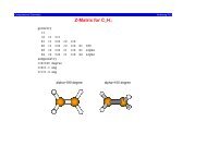
Small Molecules: newopt – zopt<br />
Optimisation of a molecule given as z-matrix using the<br />
BFGS method:<br />
newopt \<br />
function= zopt : { \<br />
zmatrix= water.zz4 \<br />
theory= mndo } \<br />
method= bfgs<br />
Johannes Kästner<br />
STFC Daresbury Lab<br />
Large Molecules: HDLCopt<br />
● Small molecule, redundant internals:<br />
hdlcopt coords=c \<br />
residues= [ res_selectall coords=c ] \<br />
theory= mndo<br />
● Large molecule, provided as pdb file, HDLCs:<br />
set residues [ pdb_to_res 1PBE.pdb ]<br />
hdlcopt coords=c \<br />
residues= $residues \<br />
constraints= {{bond 3 5} {angle 3 5 6}} \<br />
theory= mndo<br />
Johannes Kästner<br />
STFC Daresbury Lab<br />
8
Dimer Method for TS search<br />
● Dimer: two images of the system,<br />
constant distance<br />
● Rotation: difference of the forces<br />
● Movement:<br />
− In dimer direction: against the force<br />
− Perpendicular to dimer direction:<br />
along the force<br />
● Converges to first-order saddle points<br />
● No Hessian required: for large systems<br />
Johannes Kästner<br />
STFC Daresbury Lab<br />
Dimer method in <strong>ChemShell</strong><br />
dimer coords=c mode=3 \<br />
maxcyc=100 \<br />
theory= gamess : $gamess_args<br />
Johannes Kästner<br />
STFC Daresbury Lab<br />
9
Outlook: Nudged Elastic B<strong>and</strong><br />
● Multiple images, connected by “springs”<br />
● Converges to the minimum-energy path<br />
● Climbing image: transition state<br />
● Evolved, but can cover difficult reactions<br />
● Implementation in <strong>ChemShell</strong> is in “beta stage”<br />
Johannes Kästner<br />
STFC Daresbury Lab<br />
Exploiting QM/MM capabilities:<br />
Micro-iterative QM/MM optimisation<br />
One QM step<br />
Complete MM<br />
optimisation<br />
● Electrostatic embedding: ESP charges<br />
calculated on the fly<br />
● Optimisation effort becomes independent of<br />
the system size<br />
● Saves a factor of 2–10 in CPU time<br />
● hdlcopt<br />
inner_atoms= { 1 2 14 15 } mcore=true<br />
Kästner, S. Thiel, Senn, Sherwood, W. Thiel,<br />
J. Chem. Theory Comput. online (2007)<br />
Johannes Kästner<br />
STFC Daresbury Lab<br />
10
Molecular <strong>Dynamics</strong> in <strong>ChemShell</strong><br />
NVE, NVT, NPT,<br />
constant friction<br />
MD driver<br />
from DL_POLY<br />
Rigid body motion<br />
(quaternions)<br />
Monte Carlo<br />
sampling<br />
Distance <strong>and</strong><br />
other constraints<br />
(SHAKE)<br />
Johannes Kästner<br />
STFC Daresbury Lab<br />
11
Free-Energy Methods I<br />
● Fixed constraint<br />
− Thermodynamic integration: sampling the mean force<br />
● Continuously changing constraint<br />
− Slow growth: sampling the mean force<br />
− Fast growth: fast changing constraint, exponential<br />
average of the energy change<br />
● Free-energy perturbation: instantaneous changes,<br />
exponential average of the energy change<br />
Johannes Kästner<br />
STFC Daresbury Lab<br />
Free-Energy Methods II<br />
● Fixed restraint (bias)<br />
− Umbrella sampling: sampling the distribution of the<br />
reaction coordinate<br />
● Continuously changing restraint<br />
− Steered molecular dynamics<br />
● Hessian: quadratic approximation, anharmonicities<br />
neglected<br />
● …<br />
Johannes Kästner<br />
STFC Daresbury Lab<br />
12
Umbrella Sampling<br />
● A number of windows, each <strong>with</strong> a<br />
restraint (bias) centred at different<br />
points along the reaction coordinate<br />
● Distribution along the reaction<br />
coordinate is sampled<br />
● Analysis by<br />
− WHAM or<br />
− Umbrella Integration<br />
provides the free-energy difference<br />
● Restraints available in <strong>ChemShell</strong>:<br />
bond, angle, torsion, difference between 2, 3, <strong>and</strong> 4<br />
bond lengths<br />
● Use the NHC thermostat: nosehoover=4<br />
biased potential<br />
potential energy surface<br />
Johannes Kästner<br />
STFC Daresbury Lab<br />
Thermodynamic Integration<br />
● A number of windows, each<br />
constrained to a particular value<br />
of the reaction coordinate<br />
● Shake-like constraint (Lagrange<br />
multiplier)<br />
● Force on the constraint is averaged<br />
● Integration of these mean forces<br />
provides an approximate free-energy<br />
change<br />
● Metric tensor corrections<br />
● Constraints available in <strong>ChemShell</strong>:<br />
bond, torsion, difference between 2<br />
bond lengths<br />
constrained to this value<br />
potential energy surface<br />
Johannes Kästner<br />
STFC Daresbury Lab<br />
13
Exploiting QM/MM functionality:<br />
QM/MM-FEP<br />
Reaction profile:<br />
● Full QM/MM<br />
calculations<br />
● QM <strong>and</strong> MM atoms<br />
optimized<br />
Sampling:<br />
● Frozen QM part<br />
● MM-dynamics<br />
∆A = ∆E<br />
+ ∆A<br />
qm<br />
qm/mm<br />
Zhang, Liu, Yang J. Chem. Phys. 112, 3483 (2000)<br />
Johannes Kästner<br />
STFC Daresbury Lab<br />
System Preparation<br />
14
Setup of QM/MM calculations of proteins<br />
Starting point: pdb file<br />
Check errors: What If<br />
Add hydrogen<br />
Pronation state (PropKa)<br />
Solvate the protein in water<br />
Equilibrate solvate<br />
Equilibrate the whole (MM) system<br />
Structure optimisation at the QM/MM level<br />
Johannes Kästner<br />
STFC Daresbury Lab<br />
Fluorinase: Setup<br />
QM/MM setup:<br />
● Solvated in a 25 Å water sphere<br />
● QM method: DFT (BP86) <strong>with</strong><br />
Turbomole<br />
● MM method: CHARMM force<br />
field <strong>with</strong> DL_POLY in<br />
<strong>ChemShell</strong><br />
● Electrostatic embedding<br />
(charge shift)<br />
● HDLCopt, shell of 8 Å around<br />
the active site optimized<br />
Senn, O’Hagan, Thiel J. Am. Chem. Soc. 127, 13643 (2005)<br />
Johannes Kästner<br />
STFC Daresbury Lab<br />
15
Conclusions<br />
Optimisation:<br />
● Small molecules: newopt – zopt<br />
● Large systems: HDLCopt (possibly micro-iterative)<br />
Free-energy sampling:<br />
● Umbrella sampling (NHC thermostat)<br />
Further information:<br />
www.chemshell.org/manual<br />
www.chemshell.org/tutorial<br />
Johannes Kästner<br />
STFC Daresbury Lab<br />
16