High Frequency Traders, News and Volatility - HEC Paris

Fast and Slow Informed Trading ∗
Ioanid Roşu †
September 12, 2014
Abstract
This paper develops a model in which traders continuously process costly information,
and may differ in their trading speed. In equilibrium, (i) the fast informed traders (FTs)
generate most of the volatility and trading volume in the market; (ii) they must use their
information quickly, as the value of information decays fast; (iii) when the number of FTs
increases, price volatility, trading volume and liquidity increase; (iv) when the FTs’ signal
precision increases, volatility and volume increase, while liquidity decreases. FTs can
manage their inventory almost infinitely fast, but only in the presence of slower informed
traders.
Keywords:
Trading volume, inventory, volatility, high frequency trading, price impact,
Kyle model.
∗ Earlier versions of this paper circulated under the title “High Frequency Traders, News and Volatility.”
The author thanks Kerry Back, Laurent Calvet, Thierry Foucault, Johan Hombert, Pete Kyle, Stefano Lovo,
Victor Martinez, Dimitri Vayanos, Jiang Wang; finance seminar participants at HEC Paris, Durham, Leicester,
Paris Dauphine, Copenhagen, Madrid Carlos III, ESSEC; and conference participants at the European Finance
Association meetings in Lugano, American Finance Association meetings in San Diego, Society for Advancement
of Economic Theory in Portugal, Central Bank Microstructure Conference in Norway, Market Microstructure
Many Viewpoints Conference in Paris for valuable comments.
† HEC Paris, Email: rosu@hec.fr.
1

1 Introduction
Today’s markets are increasingly characterized by the continuous arrival of vast amounts of
information. A media article about high frequency trading reports on the hedge fund firm
Citadel: “Its market data system, for example, contains roughly 100 times the amount of information
in the Library of Congress. [...] The signals, or alphas, that prove to have predictive
power are then translated into computer algorithms, which are integrated into Citadel’s master
source code and electronic trading program.” (“Man vs. Machine,” CNBC.com, September
13 th 2010). The sources of information from which traders obtain these signals usually include
company-specific news and reports, economic indicators, stock indexes, prices of other securities,
prices on various other trading platforms, limit order book changes, as well as various
“machine readable news” and even “sentiment” indicators. 1
At the same time, financial markets have seen in recent years the spectacular rise of
algorithmic trading, and in particular of high frequency trading. 2
This coincidental arrival
raises the question whether or not at least some of the HFTs do process information and trade
very quickly in order to take advantage of their speed and superior computing power. Recent
empirical evidence suggests that this is indeed the case. 3
But, despite the large role played
by high frequency traders (HFTs) in the current financial landscape, there has been relatively
little progress in explaining their strategies in connection with information processing.
particular, we list a set of questions that a theoretical model about informed HFTs should
address: (i) What are the optimal trading strategies of HFTs who process information (ii)
Why do HFTs account for such a large share of the trading volume (iii) What explains the
race for speed among HFTs What are the effects of HFT on measures of market quality,
such as liquidity and price volatility (v) What explains the low inventory of at least some of
the HFTs 4
In this paper, we provide a theoretical model of informed trading which parsimoniously
addresses the questions mentioned above. In our model, informed traders called “speculators”
(i) learn gradually about the value of a risky asset (i.e., obtain “signals”), (ii) pay an
information processing cost per individual signal per trading round, and (iii) may differ in
their speed of information processing. Our main results are: (a) there is an exponential decay
1 “Math-loving traders are using powerful computers to speed-read news reports, editorials, company Web
sites, blog posts and even Twitter messages—and then letting the machines decide what it all means for the
markets.” (“Computers That Trade on the News,” New York Times, December 22 nd 2010).
2 Hendershott, Jones, and Menkveld (2011) report that from a starting point near zero in the mid-1990s,
high frequency trading rose to as much as 73% of trading volume in the United States in 2009. Chaboud,
Chiquoine, Hjalmarsson, and Vega (2014) consider various foreign exchange markets and find that starting
from essentially zero in 2003, algorithmic trading rose by the end of 2007 to approximately 60% of the trading
volume for the euro-dollar and dollar-yen markets, and 80% for the euro-yen market.
3 See Brogaard, Hendershott, and Riordan (2014), Baron, Brogaard, and Kirilenko (2014), Kirilenko, Kyle,
Samadi, and Tuzun (2014), Hirschey (2013), Benos and Sagade (2013).
4 In their analysis of the Flash Crash of May 2010, Kirilenko, Kyle, Samadi, and Tuzun (2014) define HFTs
by both high trading volume and low inventory, both at the end of the day and intraday.
In
2

of the benefits that arise from each signal, and this decay is faster with more competition
among speculators; thus, information decays quickly, which generates a need for speed; (b) as
a consequence, speculators trade only on their most recent signals; (c) by focusing disproportionately
on their most recent signals, speculators generate a very large trading volume;
(d) such a large trading volume is possible because competition among speculators ultimately
makes the market more efficient and liquid; (e) if, in addition, certain traders want to manage
their inventories, they can reduce it to zero almost infinitely fast (in “real time”) and still
make a profit, but only if other speculators trade more slowly.
More specifically, we setup our model as in Kyle (1985), but with multiple informed traders
and a changing fundamental value, v t , modeled as a diffusion process. The speculators observe
identical signals of the form ∆v t + noise, but some speculators may observe the signal with
a lag.
Along with the signal, we assume that the speculator must also learn the public’s
expectation about the signal, so that he can trade on the difference—the “non-stale” part of
the information. 5 As the public’s expectation of a signal changes after each trading round, we
assume the speculator must pay the cost each time the signal is used. Thus, signals must be
processed individually both in the cross section (different increments) and in the time series
(different trading rounds). 6
The individual signal processing cost may be in practice very
small, but as long as it is not zero, with an exponential decay of information the cost poses a
constraint that soon becomes binding.
Thus, any positive signal processing cost is enough to stop the Holden and Subrahmanyam
(1992) phenomenon, by which N > 1 informed traders with identical information release the
information so fast that no equilibrium exists in the limit when the number of trading periods
approaches infinity. In our model, the information cost “tames” the equilibrium by making
the speculators optimally forget signals which are older than a threshold.
The key intuition of our model can be grasped from a simple version of the model in which
N equally fast speculators use only their most recent signal in deciding how to trade. Then, in
each trading round t, the N speculators submit their market orders along with noise traders.
The risk neutral competitive dealer sets the price as a linear function of the aggregate order
size. Then, as in the Kyle (1985) model, each speculator faces a Cournot-type problem: he
gets benefits that are proportional to the quantity submitted (which in turn is proportional to
his signal), but faces a quadratic cost (the price impact) which increases with the aggregate
quantity. As in the Cournot model, each speculator behaves in equilibrium like a monopolist
against the residual demand curve—or, more appropriately in our context, like a monopsonist
5 In fact, even observing the signal ∆v for the first time is in practice likely to involve removing its public
expectation, so that only its orthogonal (non-stale) part can be used.
6 This assumption implicitly means that traders cannot costlessly rely on public signals such as the price to
shortcut the learning process. In the Kyle (1985) model, the price is the unique source of information about
the public’s expectations, and the speculator knows his information to be superior to that of the public’s along
all dimensions. If, instead, as it is likely in practice, an asset’s value has other components that the market
learns about, a speculator is potentially adversely selected when using the public price to decide his strategy.
3

against the residual supply curve.
As a result, each speculator trades such that the price
impact of his order is on average 1/(N + 1) of his signal. That brings the expected aggregate
price impact to N/(N + 1) of the signal, and leaves on average only 1/(N + 1) of the signal
unknown to the dealer.
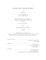
Figure 1: Profit from Lagged Signals. The figure plots the percentage of a speculator’s
profit from each his lagged signals when there is competition among N ∈ {1, 2, 3, 5, 20, 100} identical
speculators. In these examples, the speculators can trade up to m = 5 lagged signals.
100%
N = 1
100%
N = 2
100%
N = 3
80%
80%
80%
profit
60%
40%
profit
60%
40%
profit
60%
40%
20%
20%
20%
0%
0 1 2 3 4 5
lag
0%
0 1 2 3 4 5
lag
0%
0 1 2 3 4 5
lag
100%
N = 5
100%
N = 20
100%
N = 100
80%
80%
80%
profit
60%
40%
profit
60%
40%
profit
60%
40%
20%
20%
20%
0%
0 1 2 3 4 5
lag
0%
0 1 2 3 4 5
lag
0%
0 1 2 3 4 5
lag
In our dynamic model, the outcome of the trading game is more complicated, but the
basic intuition of the one-period model carries through. Namely, as soon as speculators learn
new information, they must trade very quickly, because even after one trading round only
a small fraction of the signal is left available for subsequent trades. In the next round, the
speculators exploit the new signal in a similar fashion, but in addition they can use old signals
as well. However, if a speculator uses an old signal, the same revelation mechanism only leaves
a small fraction of the small fraction already left. Hence, the benefits from repeatedly trading
on a particular signal decrease at a rate equal to 1/(N + 1) with each trading round. Thus,
with benefits decreasing at such a high rate, even a tiny information processing cost is enough
to ensure that speculators only use their most recent signals. 7
Figure 1 provides a graphic
illustration of this phenomenon when N = 1, 2, 3, 5, 20, 100 identical speculators compete for
information and use only their 5 most recent signals. Indeed, one sees that the fraction of
7 Without information processing costs, it turns out that these signals are used ad infinitum, and the
equilibrium unravels. This is in essence the Holden and Subrahmanyam (1992) effect: as the number of trading
rounds becomes very high, information revelation is almost instantaneous, the market is almost infinitely liquid,
and the equilibrium breaks down in the limit.
4

speculator profits that occur from their most recent signal is high even when N is relatively
low.
The same intuition works when comparing the fastest traders (FTs)—i.e., the speculators
that observe new signals immediately,—with the slower traders (STs), that observe signals
with a lag. When the number of FTs is sufficiently high, the profits of STs are very small.
This is because STs can trade only on old signals, and, as we discussed before, these signals
lose quickly most of their value. In addition, STs must compete with the FTs, who also trade
on their older signals. This further decreases the profits of STs. 8 Thus, FTs dominate trading
volume, hence our findings are driven mostly by the activities of FTs.
Once the basic intuition that drives our model is clear, our main results follow in a relatively
straightforward manner. Nevertheless, it is worth noting that these results are not obvious
ex ante. In particular, the literature on informed trading has had difficulties attributing the
high trading volume observed in practice to informed traders. Indeed, Kyle (1985), Back and
Pedersen (1998), or Back, Cao, and Willard (2000), as the number of trading rounds is high
(and in the continuous time limit) the speculators generate only a tiny fraction of the trading
volume, as speculators trade smoothly on their long-lived information. By contrast, in our
model FTs trade aggressively only on their most recent signals and ignore information that is
too old. As a result, informed trading in our model occurs in a noisy fashion, essentially as
noisy as the information received by the FTs. Thus, paradoxically, an information processing
cost dissuades even a single speculator from trading smoothly on long-lived information, and
instead drives FTs to reveal a large part of their signals almost instantly.
Quantitatively,
the aggregate FT trading volume can be shown to increase almost linearly in N, and the FT
participation rate is of the order of N/(N + 1) as a fraction of the overall trading volume.
The reason why FT trading volume can be so high is that in equilibrium the market is very
liquid, and FTs can trade without much price impact. Indeed, quick information revelation
makes the market close to strong-form efficient and hence very liquid. The dealer knows that
most of the information is eventually released by the speculators, and endogenously chooses a
small price impact for trading. This creates an amplification mechanism that provides ample
room for trading.
The effect of FTs on volatility is more muted. In our model, it turns out that the price
volatility is bounded above by the fundamental volatility of the asset.
Nevertheless, price
volatility increases with FT competition and signal precision. The intuition is that as FTs
trade more aggressively, they release most of their information, so that in the limit the market
becomes strong-form efficient, and price volatility equals fundamental volatility.
One of the most puzzling aspects of high frequency trading is the quick turnaround of HFT
positions, i.e., the maintenance of very low HFT inventories. Kirilenko, Kyle, Samadi, and
8 Baron, Brogaard, and Kirilenko (2014) study the profits of HFTs and find out that, in agreement with
our model, HFT profits are concentrated among a small number of incumbents.
5

Tuzun (2014) report that HFTs in their sample liquidate 0.5% of their aggregate inventories
on average each second, implying HFT inventories have an AR(1) half-live of a little over
2 minutes. To study this problem, we allow a subset of the speculators—called HFTs—to
manage their inventory. We find that in our model HFTs can manage their inventories almost
infinitely fast, while still maintaining positive average profits. This, however, can be done only
if there exist “slow” traders. By “slow” traders we mean either (i) STs, who are genuinely slow
and can only trade on older information; or (ii) FTs who also trade on their older information
(lagged signals) because it is optimal for them to do so. To understand the intuition for this
result, consider a FT who trades on his information. In the absence of inventory management,
the inventory of the FT represents an accumulation of signals which are positively correlated
with the asset value. By trading to lower his inventory, the FT trades against his information,
and if he does this too fast, he may eventually trade at a loss. However, we show that by
selling the asset at the same time that other speculators are buying, the FT may lower his
price impact, and, if the inventory management is done properly, the FT can maintain positive
profits. This is true even if the chosen mean-reversion rate is virtually infinite.
Related Literature
Our main intuition regarding the quick information decay when informed traders compete
is also present in Foster and Viswanathan (1996). They find that informed traders with
correlated signals engage in a “rat race,” and reveal their common information very fast.
Furthermore, in the extreme case when informed traders have identical signals, Holden and
Subrahmanyam (1992) find that, as the number of trading rounds increases, the signal is
revealed almost instantaneously, such that in the continuous time limit there cannot be any
equilibrium in smooth strategies, as in Kyle (1985). If the signals are not identical, however,
Foster and Viswanathan (1996) show that the rat race is followed by a “waiting game,” in which
traders reveal their information very slowly, as they are likely to be on the opposite side of a
trade. Back, Cao, and Willard (2000) confirm that the equilibrium in smooth strategies with
the rate race and waiting game survives in a continuous time setup. Our paper contributes to
this literature by showing that even a tiny information processing cost slows down the rat race
enough so that the equilibrium survives even when the number of trading rounds becomes very
large (at the “high frequencies”). Nevertheless, in our equilibrium strategies are not smooth as
in Kyle (1985), but they are volatile and place a large weight on traders’ most recent signals.
In the papers mentioned above, the signals are static, as they are received only at the
beginning of the trading game. A more recent literature investigates the effect of dynamic
signals, by which traders gradually learn over time. Back and Pedersen (1998) extend the
basic setup of Kyle (1985) to allow for dynamic signals, and find that in equilibrium the
insider continues to have smooth strategies. In their model, as in Kyle (1985), the insider
6

places the same weight on all the past signals and thus trades on the aggregate signal, which
is his forecast of the fundamental value.
In Chau and Vayanos (2008), the strategies are
similar, but at high frequencies (i.e., when the time between trading rounds becomes very
small) the insider trades with almost infinite weight and the market approaches strong-form
efficiency. 9 This perhaps should not be surprising if one interprets Chau and Vayanos (2008)
as a stationary version of Back and Pedersen (1998). Indeed, in Back and Pedersen (1998),
as in Kyle (1998), the market approaches strong-form efficiency towards the liquidation date,
and the insider trades almost with infinite weight. 10
By contrast, in our paper speculators
trade only on their most recent signals, and the market is not strong-form efficient (although it
becomes so in the limit when the number of speculators is large). One other paper that breaks
the symmetry among past signals is Foucault, Hombert, and Roşu (2013). In their model, a
single speculator receives a signal one instant before the public, and as a result, trades with
a large weight on the last signal (the “news”). In their model, the value of information is lost
quickly because of public news. In our model, it decays quickly because of competition among
informed traders.
Our paper is part of a growing theoretical literature on High Frequency Trading. 11
much of this literature, it is the speed difference that has a large effect in equilibrium. The
usual model setup has certain traders who are faster in taking advantage of an opportunity
that disappears quickly. As a result, traders enter into a winner-takes-all contest, in which
even the smallest difference in speed has a large effect on profits. (See for instance the model
of “sniping” of Budish, Cramton, and Shim (2014), or the model of news anticipation of
Foucault, Hombert, and Roşu (2013).) By contrast, our main results remain true even if all
informed traders have the same speed. This is because in our model the need for speed arises
endogenously, from competition among informed traders. In our model, being “slow” simply
means trading on older signals. Since in equilibrium speculators also use older signals (the
unanticipated part of the signals, to be precise), in some sense all traders are slow as well.
Nevertheless, it is true that a genuinely slower trader makes less money in our model, since
he can only trade on older information that has already lost much of its value.
The paper is organized as follows. Section 2 describes the model. Section 3 solves the
model with two classes of informed traders: fast and slow.
In
Section 4 discusses empirical
implications of the model regarding the effect of fast traders on various measures of market
quality. Section 5 analyzes the inventory management of speculators. Section 6 discusses the
equilibrium in the general case, as well as robust trading strategies, which are strategies that
9 Li (2012) confirms Chau and Vayanos (2008) in an extension with multiple traders. He also finds that
because of competition informed trading volume increases by an order of magnitude.
10 Caldentey and Stacchetti (2010) find that a random liquidation deadline has essentially the same effect as
the stationarity in the Chau and Vayanos (2008) model.
11 See Budish, Cramton, and Shim (2014), Biais, Foucault, and Moinas (2014), Foucault, Hombert, and Roşu
(2013), Pagnotta and Philippon (2013), Aït-Sahalia and Saglam (2014), Li (2014), Weller (2013), Hoffmann
(2013), Cartea and Penalva (2012), Jovanovic and Menkveld (2012).
7

simplicity 12 T = 1. (1)
perform well under alternative specifications of the model. Section 7 concludes. All proofs are
in the Appendix or the Internet Appendix.
2 The Model
2.1 Setup
Trading for a risky asset takes place continuously over the time interval [0, T ], where for
Trading occurs at intervals of length dt apart. Throughout the text, we refer to dt as representing
either one period, or one trading round. The liquidation value of the asset is
v T =
∫ T
0
dv t , with dv t = σ v dB v t , (2)
where Bt
v is a Brownian motion, and σ v > 0 is a constant called the fundamental volatility.
We interpret v T as the “long-run” value of the asset; in the high frequency world, this can
be taken to be the asset value at the end of the trading day. The increments dv t are then
the short term changes in value due to the arrival of new information. The risk-free rate is
assumed to be zero.
There are three types of market participants: (a) N ≥ 1 risk neutral speculators, who
observe the flow of information at different speeds, as described below; (b) noise traders; and
(c) one competitive risk neutral dealer, who sets the price at which trading takes place.
Information. At t = 0, there is no information asymmetry between the speculators and
the dealer. Subsequently, each speculator receives the following flow of signals:
ds t = dv t + dη t , with dη t = σ η dB η t , (3)
where t ∈ (0, T ] and B η t
by
is a Brownian motion independent from all other variables. Denote
w t = E(v T
∣ ∣ {sτ } τ≤t ) (4)
the expected value conditional on the information flow until t. We call w t the value forecast,
or simply forecast. Since there is no information asymmetry at t = 0, we have w 0 = 0. The
increment of w t is
dw t = ads t , with a =
σ 2 v
σv 2 + ση
2 , (5)
12 To eliminate confusion with later notation, we often use T instead of 1. This way, we can denote t − dt
by t − 1 without much confusion.
8

where the parameter a is called signal precision. If we denote by σ w the instantaneous volatility
of w t , we compute
σ w =
( ) Var(dwt ) 1/2
= a
dt
( ) Var(dst ) 1/2
=
dt
σ 2 v
√
σ 2 v + σ 2 η
. (6)
As the forecast volatility σ w and the signal precision a are monotonic transformations of each
other, we use these two notions interchangeably when deriving empirical implications.
Speculators obtain their signal with a lag l = 0, 1, . . .. Thus, we define a l-speculator to
be a trader who at t ∈ (0, T ] observes the lagged signal ds t−ldt , from l periods before. For
each lag l = 0, 1, 2, . . ., denote by N l the number of l-speculators. For simplicity of notation,
henceforth we use the following convention:
Notation for trading times: t − l instead of t − ldt. (7)
For instance, we write ds t−l instead of ds t−ldt .
Trading. At each t ∈ (0, T ], denote by dx i t the market order submitted by speculator
i = 1, . . . , N at t, and by du t the market order submitted by the noise traders, which is of
the form du t = σ u dBt u , where Bt
u is a Brownian motion independent from all other variables.
Then, the aggregate order flow executed by the dealer at t is
dy t =
N∑
dx i t + du t . (8)
i=1
Because the dealer is risk neutral and competitive, she executes the order flow at a price equal
to her expectation of the liquidation value conditional on her information. Let I t = {y τ } τ

which the l-speculator’s strategy is linear in the unpredictable parts of his signals: 13
dx t = γ l,t (dw t−l − z t−l,t ) + γ l+1,t (dw t−l−1 − z t−l−1,t ) + · · · , (11)
where z t−k,t is the dealer’s expectation of dw t−k conditional on her information set at t:
z t−k,t = E ( dw t−k | I t
)
. (12)
We further assume that the speculators take the covariance structure of z t−k,t to be fixed, as
part of the dealer’s pricing rules. 14
A linear equilibrium is such that: (i) at every date t, each speculator’s trading strategy (11)
maximizes his expected trading profit (10) given the dealer’s pricing policy, and (ii) the dealer’s
pricing policy given by (9) and (12) is consistent with the equilibrium speculators’ trading
strategies.
Information Processing Cost. There is a positive information processing cost c per
individual piece of information and per unit of time. Formally, the total information cost from
date τ onwards is:
C τ =
∫ T
τ
∞∑
1 γk,t ≠0 c dt, (13)
where 1 P is the indicator function, which equals 1 if P is true, and 0 otherwise.
k=l
We do not model the exact nature of the speculators’ signals and the information processing
costs. But, intuitively, an individual information processing cost per each trading round
is plausible for several reasons. First, as explained in the Introduction, in today’s markets
traders use many high frequency sources of information to obtain their signals. In practice,
processing these signals amounts not only to estimating the absolute magnitude of the signal,
but also to measuring it relative to a public expectation. 15
Often, however, these expectations
are not readily available to the traders, and must be inferred either from observing the
order flow (by estimating how much information has already been released both via own and
competitors’ trades), and from the analysis of public news (some signals might have already
become public in the meantime). Thus, extracting the unpredictable (non-stale) part for each
piece of information, which we model as the orthogonal increment dw t , is a non-trivial task
which in practice is likely to require fast and accurate processing abilities. And once dw t is
computed and used to trade, speculators must subsequently use only the non-stale part, which
13 This type of strategies occur in virtually all models of Kyle (1985) type. In the Internet Appendix, we
show in a discrete time version of the model that these type of strategies arise naturally in equilibrium.
14 For more discussion regarding this assumption, see the proof of Theorem 1. Also, in Section 6 we explore
an alternative assumption by which speculators’ trading strategies to affect the covariances of z t−k,t . We find
that the overall effect is very small, so that our main results remain qualitatively the same.
15 For instance, one often measures earnings surprises by comparing the absolute magnitude of the earnings
announcement with the analyst consensus estimate.
10

keeps changing after each trade. 16 Given all these reasons, it is plausible to expect that in
practice an individual information processing per unit of time is necessary.
Note that the assumption of an individual processing cost means implicitly that speculators
cannot simply rely on free public signals, such as the price, to shortcut the learning process.
This is because in reality prices may contain other relevant information about the fundamental
value, along which the speculators are adversely selected. We formalize this intuition in
Section 6.3, and introduce an orthogonal dimension of the fundamental value. We show that
trading strategies that rely on prices make an average loss, while trading as in our model
remains profitable.
2.2 The Model of Trading with m Lagged Signals
Solving for the equilibrium in the general setup of Section 2.1 turns out to be challenging.
There are two main reasons for this. First, the model does not specify how many past signals
can be processed by each speculator, and this can in principle lead to multiple equilibria.
Second, as the signals are processed individually, the complexity of the problem increases
with the number of signals;
Thus, we propose the following solution technique. We consider the same setup in Section
2.1, but instead of introducing an information processing cost, we set the cost to zero, and
consider only trading strategies in which signals are used for at most an exogenously chosen
number of trading periods, m.
Assumption 1. The speculators’ trading strategies can involve only their current signal
and their most recent past m signals. More precisely, at time t, each speculator’s trading
strategy must be of the form
dx t = γ 0,t (dw t − z t,t ) + γ 1,t (dw t−1 − z t−1,t ) + γ m,t (dw t−m − z t−m,t ), (14)
where z t−k,t is the dealer’s expectation of dw t−k , given her information.
information processing cost, i.e., c = 0.
Also, there is no
To justify this assumption, we argue that a positive signal processing cost c is economically
equivalent to Assumption 1. Indeed, as we show later in Section 6, the benefit of each lagged
signal decreases exponentially with the lag. Then, given a signal processing cost c, the benefit
of each individual signal must decay below c after a large enough number of lags. At that
point, it is not worth using that signal anymore. This determines the number m of past signals
that can be profitably used.
16 Furthermore, we show below that (i) the non-stale part changes by different amounts for the different
pieces of information, (ii) the optimal weights (γ k ) are different even when speculators have the same speed,
(iii) the optimal weights depend on the signal precision, and while in the model this precision is constant, in
practice it may different from one signal to the next.
11

Throughout the paper, we refer to the modified setup in this section as the model of trading
with m lagged signals. Because the solution of this model is more involved in the general case,
we postpone its discussion until Section 6. However, as we have mentioned already, one of the
key properties of the general equilibrium is that the benefits of lagged information decay very
quickly. Thus, it turns out that most of the results in the general case can already be obtained
in the model of trading with m = 1 lagged signals. Thus, in the next section we discuss this
case in detail, and we see that its solution can be expressed in closed form.
3 Equilibrium with Fast and Slow Traders
In this section, we analyze the model of trading from Section 2.2 in which speculators can
trade with only one lagged signal (m = 1). This means that at time t speculators use only (i)
their most recent signal, dw t , if this is observed; and (ii) the signal with one lag, dw t−1 (recall
that t − 1 is notation for t − dt). Thus, there are two types of speculators:
• Fast Traders, or FTs, who observe at t both dw t and dw t−1 ;
• Slow Traders, or STs, who observe at t only dw t−1 .
To proceed with the solution, we need to be more specific about how the dealer sets her
expectation z t−k,t = E(dw t−k | {dy τ } τ

where γ S t = 0 for the slow trader. Also, denote by N F the number of FTs, and by N S the
number of STs. The total number of speculators is
N T = N F + N S . (18)
The next result shows that the model has a closed form solution.
Theorem 1. Consider the trading model with m = 1 lagged signals, with N F > 0 fast traders
and N S ≥ 0 slow traders. Then, there exists a linear equilibrium of the model with constant
coefficients, of the form (t ∈ (0, T ]):
dx F t = γdw t + µ ˜dw t−1 ,
dx S t = µ ˜dw t−1 ,
˜dw t−1 = dw t−1 − ρdy t−1 ,
(19)
dp t = λdy t ,
where the coefficients γ, µ, ρ, λ are given by:
γ = 1 λ
µ = 1 λ
1
N F + 1 ,
1 1
N T + 1 1 + b ,
√
NF
N F +1 − b
√
NT
N T +1 − ωb
ρ = σ √
w (1 − a)(a − b
σ 2 ) = σ (20)
w 1 1 + b
N
√ T
u σ u NF + 1 ω + b
N T + 1 ,
N F
λ = ρ
N F − b ,
and a ∈ (0, 1), b ∈ (0, 1) and ω ∈ (1, 2) are defined by
b =
√
ω 2 + 4 N T
N T +1
2
− ω
, with ω = 1 + 1
N F
N T
N T + 1 ,
a = N F − b
N F + 1 . (21)
One consequence of the Theorem is that FTs and STs trade with the same intensity on
their lagged signal. This turns out to be true because the new signal dw t is uncorrelated with
the lagged signal ˜dw t−1 . This result, however, does not generalize to the case when there are
more lags (see Section 6). In that case, there is autocorrelation between the signals of different
lags, which reflects a more complicated covariance structure. 18
18 In the language of Section 6, this translates mathematically into the fresh covariance matrix having non
zero entries A i,j when i > j ≥ 1.
13

The next Corollary provides asymptotic results when the number N F of FTs is large. We
say that the asymptotic value of a number X which depends on N F is X ∞ if
X
lim = 1. (22)
N F →∞ X ∞
Corollary 1. In the context of Theorem 1, if N F
the following asymptotic values:
is large, the equilibrium coefficients have
γ ∞
= σ u
σ w
1
√
NF
,
µ ∞ = σ u
σ w
1
√
NF
N F
N T
b ∞ ,
ρ ∞ = λ ∞ = σ w
σ u
1
√
NF
.
(23)
Moreover, the numbers b, a, ω approach
b ∞ =
√
5 − 1
, a ∞ = ω ∞ = 1. (24)
2
We also provide some formulas that follow from Theorem 1, which are used throughout
the text.
Corollary 2. In the context of Theorem 1, the following formulas are satisfied:
Var ( ˜dwt
)
dt
λ ¯γ =
= (1 − a) σ 2 w = 1 + b
N F + 1 σ2 w,
N F
N F + 1 , λ ¯µ = 1
1 + b
Cov ( ) ˜dwt , w t
dt
N T
N T + 1 ,
= 1 − a
1 + b σ2 w =
σw
2 (25)
N F + 1 .
We use the results in Theorem 1 to compute the expected profits of the fast traders and
the slow traders.
Proposition 1. In the context of Theorem 1, the expected profit of the FTs and STs at t = 0
from their equilibrium strategies are given, respectively, by:
π F =
π S =
γ
N F + 1 + 1
1
N F + 1
µ
N T + 1 ,
N F + 1
(26)
µ
N T + 1 .
The ratio of slow to fast profits is therefore
π S
π F = 1
1 + (N T +1) 2 (1+b)
N F +1
π S
=⇒ lim
N F →∞ π F = N F 1
(N F + N S ) 2 . (27)
1 + b ∞
14

Thus, even if there is only one ST (N S = 1), the ST profits are small compared to the
FT profits. The reason is that FTs trade also on their lagged signals, and thus compete with
the STs. Indeed, FTs compete for trading on dw t only among themselves, while they also
compete with the STs for trading on the lagged signal ˜dw t−1 .
4 Fast Traders and Market Quality
We now discuss the effect of fast trading on various measures of market quality, such as
liquidity, trading volume, price volatility, price informativeness, etc. First, we need to define
these measures in the context of our model with fast and slow traders. Suppose the market is
in the equilibrium described by Theorem 1, and the price changes according to the following
rule:
dp t = λ dy t = λ
(du t + ¯γ dw t + ¯µ ˜dw
)
t−1 , (28)
where ¯γ = N F γ is the aggregate equilibrium weights on dw t , and ¯µ = (N F + N S )µ = N T µ is
the aggregate equilibrium weight on ˜dw t−1 .
First, we define λ as the measure of illiquidity, as it is standard in the literature. Thus,
the market is considered illiquid if the price impact per unit of trade is very large, i.e., if λ is
large.
We define trading volume as the infinitesimal variance of the aggregate order flow dy t :
TV = σy 2 = Var(dy t)
. (29)
dt
We argue that this is a measure of trading volume. Indeed, in each trading round the actual
aggregate order flow is given by dy t . Thus, one can interpret trading volume as the absolute
value of the order flow: |dy t |. From the theory of normal variables, the average trading
volume is given by E ( |dy t | ) √
2
=
π σ y. With our definition TV = σy, 2 we observe that TV
is monotonic in E ( |dy t | ) , and thus TV can be used a measure of trading volume. Using the
formula dy t = du t + ¯γ dw t + ¯µ ˜dw t−1 , we compute the trading volume in our model by the
formula
TV = σ 2 u + ¯γ 2 σ 2 w + ¯µ 2 σ 2˜w , with σ2˜w = Var( ˜dwt
)
dt
. (30)
We define price volatility σ p to be the square root of the instantaneous price variance:
σ p =
( ) Var(dpt ) 1/2
. (31)
dt
From (28), it follows that the instantaneous price variance can be computed simply as the
15

product of the illiquidity measure λ and the trading volume TV = σ 2 y. Thus,
σ 2 p
= λ 2 TV = λ 2 ( σ 2 u + ¯γ 2 σ 2 w + ¯µ 2 σ 2˜w
)
. (32)
The trading volume measure TV can be decomposed into the noise trading volume and
the speculator trading volume:
TV = TV n + TV s , with TV n = σu, 2 TV s = ¯γ 2 σw 2 + ¯µ 2 σ
2˜w . (33)
The speculator participation rate is defined as the ratio of speculator trading volume over total
trading volume:
SPR = TV s
TV = ¯γ 2 σw 2 + ¯µ 2 σ 2˜w
σu 2 + ¯γ 2 σw 2 + ¯µ 2 σ 2˜w
. (34)
Note that SPR can also be interpreted as the fraction of price variance due to the speculators.
We define price informativeness as a measure inversely related to the forecast error variance
Σ t = Var ( (w t − p t−1 ) 2) . 19 Thus, if prices are informative, they stay close to the forecast w t ,
i.e., the variance Σ t is small. In Section 6, we show that in the general model of trading with
m lagged signals (Proposition 6) that Σ t evolves according to: Σ ′ t = σ 2 w − σ 2 p, where σ 2 p is the
price variance. Therefore, since Σ ′ t is inversely monotonic in the price variance, we do not use
it as a separate measure of market quality.
The next result gives explicit formulas for our measures of market quality. As before, we
use the following asymptotic notation when N F is large: X ≈ Y stands for
X
lim
N F →∞
Y = 1.
Proposition 2. Consider the setup of Theorem 1 with N F fast traders and N S slow traders.
Then, the price impact coefficient, trading volume, price volatility, and speculator participation
rate satisfy
λ = σ w
σ u
√
(1 + b)(a − b 2 )
√
NF + 1
N F
N F − b ≈ σ w
σ u
1
√
NF
,
TV = σu(N 2 a
F + 1)
(1 + b)(a − b 2 ) ≈ σ2 u (N F + 1),
(
σp
2 = σw
2 1 − N )
F (1 − b) − b
≈ σ 2
(N F + 1)(N F − b)
w,
(35)
SPR = a + b2 (1 + b)
N F − b
≈ 1.
For comparison, we solve the trading model with m = 0 lags, and compute the corresponding
market quality measures.
Proposition 3. Consider the case with N fast traders who can only use their last signal
19 See the definition in equation (62) for the general case with m lagged signals.
16

(m = 0), i.e., their trading strategy is of the form dx t = γ t dw t . Then, the coefficient γ of the
optimal strategy satisfies:
γ = 1 λ
1
N + 1 = σ u
σ w
1
√
N
. (36)
Also, the price impact coefficient, trading volume, price volatility, and speculator participation
rate satisfy:
λ = σ w
σ u
TV = σ 2 u(N + 1),
√
N
N + 1 = √ a σ v
σ u
√
N
N + 1 ,
(37)
σp
2 = σw
2 N
N + 1 = N
aσ2 v
N + 1 ,
SPR =
N
N + 1 .
We see that Proposition 3 and 2 produce qualitatively similar results, showing that the fast
traders dominate the market quality measures. We thus discuss the empirical implications of
Proposition 3, knowing that they are robust to the existence of slower traders.
We now discuss the effect of an increase in the number N of FTs on the market quality
measures. An important consequence of Proposition 3 is that in our context, the speculator
participation rate can be made arbitrarily close to 1 if the number N of FTs is large. Thus,
noise trading volatility need only be a small part of the total volatility. This stands in sharp
contrast for instance with the models of Kyle (1985) or Back, Cao, and Willard (2000), in which
at the very high frequency (in continuous time) virtually all instantaneous price volatility is
generated by noise traders.
Also, note that the market is more efficient when N is large. Indeed, Proposition 6 implies
that the rate of change of the forecast error variance Σ ′ is constant and equal to σ 2 w − σ 2 p, and
therefore Σ 1 = σ 2 w − σ 2 p as well (we have assumed Σ 0 = 0). In our case, Proposition 3 implies
that Σ ′ = σ2 w
N+1 , which implies that Σ t ≤ σ2 w
N+1 for all t. In other words, Σ t is close to zero at all
times, which means that prices stay close to fundamentals at all times. Thus, a larger number
N of FTs, rather than destabilizing the market, make the market in fact more efficient.
The trading volume TV strongly increases with the number N of FTs. 20
This occurs
because of the competition among FTs make them trade more aggressively. At the same time,
by trading more aggressively, they reveal more information which, as we see below, also lowers
the price impact. This has an amplifier effect on the trading aggressiveness, to the point that
the trading volume grows essentially linearly in the number of speculators, as can be seen
from Proposition 3. The speculator participation rate SPR also increases in N, since SPR is
20 This is also true when more lagged signals are used (m > 1), and all speculators have equal speed. Indeed,
in this case Proposition 7 implies that TV = σ 2 u(N + 1) as well.
17

the fraction of trading volume caused by the speculators.
Surprisingly, a larger number of FTs make the market more liquid, as more information
is revealed when there are more competing speculators. This appears to be in contradiction
with the fact that more informed trading should increase the amount of adverse selection. To
understand the source of this apparent contradiction, note that illiquidity is measured by the
price impact λ of one unit of volume. But, while the volume of trading TV strongly increases
in N in an unbounded way, at the same time the price impact is bounded by magnitude of the
signal dw t . 21 Thus, the price impact per unit of volume may actually decrease, and in fact it
does in our case, as prices are overall more informative. This makes the market more liquid,
hence λ decreases. This is consistent with the empirical studies of Zhang (2010), Hendershott,
Jones, and Menkveld (2011), and Boehmer, Fong, and Wu (2014).
To understand the effect of N on the price volatility σ p , recall the pricing formula dy t =
λdy t which implies σp 2 = λ 2 TV . Thus, there are two effects of N on the price volatility σ P .
First, the trading volume TV strongly increases in N, which has a positive effect on σ P .
Second, price impact λ decreases in N, which has a negative effect on σ P . The first effect is
slightly stronger than the second, thus on net price volatility σ P increases in N. This result
is consistent with the empirical studies of Boehmer, Fong, and Wu (2014) and Zhang (2010).
A few caveats are in order. First, all these studies analyze the effects of HFT activity,
where activity is proxied either by turnover or by intensity of order-related message traffic,
and not by the number of HFTs present in the market. An answer to this concern is that,
as we have seen, trading volume does increase in N. Second, in our paper we do not model
passive HFTs, that is, HFTs that offer liquidity via limit orders. Therefore, it is quite possible
that an increase in the number of passive HFTs decreases price volatility, which would cancel
the opposite effect of the number of active HFTs. For instance, Hasbrouck and Saar (2012)
document a negative effect of HFTs on volatility, possibly due to the fact that they also
consider passive HFTs, which by providing liquidity have a stabilizing effect on price volatility.
Moreover, Chaboud, Chiquoine, Hjalmarsson, and Vega (2014) find essentially no relation. In
our model, the dependence of price volatility on N is weak, which may explain the different
results in the empirical literature.
We now discuss how the various measures of market quality depend on the FTs’ signal
precision a. An interesting consequence of Proposition 3 is that the signal precision a and the
fundamental volatility σ v do not affect the market quality separately, but only via the product
σ w = √ aσ v . In what follows, we discuss only the results regarding the signal precision, but
those results apply equally to the fundamental volatility.
The price volatility σ p increases in the FTs’ signal precision a. Indeed, σ p is the volatility
of dp t , which is the price impact of the aggregate order flow. In particular, the order flow
21 See the discussion surrounding Proposition 9, which makes this intuition more rigorous in the general case.
18

coming from FTs has an aggregate price impact of λ Nγdw t =
N
N+1 dw t. 22 But the volatility
of this is proportional to σ 2 w = aσ 2 v, which is proportional to the signal precision. Hence, σ p
increases in the signal precision a, and so does the speculator participation rate SPR.
Signal precision a increases adverse selection between FTs and the dealer, hence it increases
the illiquidity λ. Trading volume TV is independent of a. To get some intuition for this result,
note that TV = σ2 p
λ 2 . Since both the numerator and denominator increase with signal precision,
the net effect is not clear. Indeed, in the context of Proposition 3, the two effects exactly offset
each other.
We now discuss the autocorrelation of order flow. Brogaard (2011) finds empirically that
the autocorrelation of aggregate HFT order flow is small but positive. We find that in our
theoretical model the aggregate speculator order flow has a positive serial autocorrelation.
To understand why, we consider our baseline model with fast and slow traders. Denote the
aggregate speculator order flow by
d¯x t = ¯γdw t + ¯µ ˜dw t−1 , with ¯γ = N F γ, ¯µ = N T µ, (38)
where ¯γ and ¯µ are the aggregate equilibrium coefficients on the signals. Since ˜dw t = dw t −ρdy t ,
the order flow serial autocorrelation has two components:
Cov ( dx t , dx t+1
)
Var(dx t )
= ¯µ¯γ Cov( dw t , ˜dw
)
t
Var(dx t )
= ¯µ¯γ Cov( )
dw t , dw t
Var(dx t )
+ ¯µ 2 Cov( ˜dwt−1 , ˜dw t
)
Var(dx t )
+ ¯µ 2 Cov( ˜dwt−1 , −ρ¯µ ˜dw
)
t−1
.
Var(dx t )
Thus, order flow autocorrelation occurs for two reasons: (i) there is a positive correlation
between the new signal of FTs at t (dw t ) and the lagged signal of both the FTs and STs at
t + 1 ( ˜dw t ); (ii) there is a negative correlation between the lagged signal at t ( ˜dw t−1 ) and the
lagged signal at t + 1 ( ˜dw t = dw t − ρdy t ), due to the negative expectation adjustment of dw t
at t + 1.
Proposition 4. In the context of Theorem 1, the speculator order flow serial autocorrelation
is:
Corr ( dx t , dx t+1
)
=
b(b + 1)(a − b 2 )
a 2 + b 2 (1 − a)
1
N F + 1 ≈
(39)
b ∞
N F
. (40)
where b ∞ =
√
5−1
2
= 0.618.
Thus, in the model the speculator order flow autocorrelation is low, yet positive. For
instance, with N F = 20 FTs, the speculator order flow autocorrelation is approximately 3%.
This result is consistent with the empirical literature on HFTs (see Brogaard (2011)). To
get some intuition, note that order flow autocorrelation arises from speculators’s signals this
22 See the equation for γ in Proposition 3.
19

period being correlated with their lagged signals next period. However, when the number of
1
FTs is large, there is only
N F +1
of the signal left to traders for the next period. Hence, one
1
should expect the autocorrelation to decrease by the order of
N F +1
, which is indeed the case.
5 Inventory Management
In this section, we show that the fast traders can manage their inventory extremely quickly,
but only in the presence of slower traders. To get some intuition, consider the model with fast
and slow traders from Section 3. For simplicity, we take a partial equilibrium approach and
assume that a subset of the FTs decides to manage their inventory by adding a mean-reverting
component to their trading strategy, as described below. To distinguish these traders from the
regular FTs, we call them High Frequency Traders, or HFTs in short. This is indeed consistent
with Kirilenko et al. (2014), who include in the definition of HFTs the condition of having a
low inventory.
We find that essentially there are two regimes of inventory management. In the first
regime, called the smooth regime, inventories mean revert to zero after a relatively long time.
In the second regime, called the extreme regime, inventories can mean revert to zero after
an infinitesimal amount of time (of the order of dt). In both cases, we show that inventory
management can be done such that profits remain positive, but this is true only if there exist
slower traders.
Thus, in the smooth regime we assume that HFTs have a trading strategy of the form: 23
dx HFT
Sm,t = −θx t−1 dt + γ ∗ dw t . (41)
With this definition, the HFT’s inventory x t becomes a regular Ornstein–Uhlenbeck process,
which is the generalization of an AR(1) process to continuous time.
In the extreme regime we assume that HFTs have a trading strategy of the form
dx HFT
Ex,t = −Θx t−1 + γ ∗ dw t . (42)
With this definition, the HFT’s inventory x t becomes an actual AR(1) process, only that
everything happens in very rapid succession.
The main difference is that this time there
is no “dt” term that multiplies the inventory x t−1 . In other words, in the extreme regime
the mean reversion coefficient (Θ) is an order of magnitude ( 1 dt
times) larger than the mean
reversion coefficient in the smooth regime (θdt). Interestingly, even under extreme inventory
management, all the relevant variables are well defined, including the expected profit of the
HFTs. Normally, one should expect that the extreme inventory management erodes the HFT
23 To obtain simpler formulas, we have assumed that HFTs do not use any lagged signals. We have also
worked out the case in which HFTs use lagged signals as well, and the qualitative results are the same.
20

profits to the point where they become negative. But it turns out that losses can be prevented
if there exist also slower traders.
Note that in the extreme regime we can write the HFT inventory in autoregressive form:
x t = (1 − φ)x t−1 + γ ∗ dw t , with φ = 1 − Θ. (43)
With the usual definition, the half life of the inventory is then defined as ln(1/2)
ln(φ)
. This by
definition is the average number of trading rounds that the process needs to halve the distance
from its mean. Since a period in our model is of length dt, the inventory half life satisfies:
Inventory Half Life Extreme
= ln(1/2)
ln(φ)
dt. (44)
This is the sense in which HFTs in our model can do “real-time” inventory management.
Depending on how dt is interpreted in practice, the inventory half life can be a few seconds,
milliseconds or even microseconds.
By contrast, in the smooth regime, the autoregressive coefficient is 1 − θdt, which gives
the following formula
Inventory Half Life Smooth = ln(1/2)
ln(1 − θdt)
ln(2)
dt = . (45)
θ
Note that, indeed, the inventory half life in the smooth regime is one order of magnitude
higher than in the extreme regime.
The next result analyzes the expected profits of the HFTs in the two inventory management
regimes.
Theorem 2. Consider the model from Section 3, to which we add N I HFTs. These have a
trading strategy engage in inventory management, as described above, using either the smooth
regime or the extreme regime. Suppose ¯γ and ¯µ are the aggregate speculator coefficients on
dw t and ˜dw t−1 , respectively, and ρ and λ are the dealer’s pricing coefficients. (These numbers
need not take the equilibrium values.)
In the smooth regime, the expected profit of a HFT (at t = 0) satisfies:
π HFT
Sm,θ
σ 2 w
=
( )
γ ∗ − λγ ∗¯γ e −θt 1 − ρ¯γ
+ λ¯µγ ∗
1 + ρ¯µ
λγ 2 ∫ 1 (
∗
− N I
1 − e
−2θt ) dt.
2(1 + ρ¯µ)
0
∫ 1
0
(
1 − e
−θt ) dt
(46)
This expression has a limit when θ → ∞:
πSm,θ
HFT
lim
θ→∞ σw
2
1 − ρ¯γ
= λ¯µγ ∗
1 + ρ¯µ − N λγ∗
2 I
2(1 + ρ¯µ) . (47)
21

In the extreme regime, the expected profit of a HFT satisfies:
π HFT
Ex,Θ
σ 2 w
1 − ρ¯γ
= λ¯µγ ∗
1 + φρ¯µ − N λγ∗
2 I
, with φ = 1 − Θ. (48)
(1 + φ)(1 + φρ¯µ)
Furthermore, the profits in the two regimes are continuous across regimes, i.e.,
lim
θ→∞ πHFT Sm,θ
= lim
Θ→0
π HFT
Ex,Θ. (49)
Theorem 2 shows that the HFT profits vary continuously under the two inventory management
regimes. With no inventory management (θ = 0), the profits satisfy the usual formula,
π HFT
Sm,θ = ( γ ∗ − λγ ∗¯γ ) σ 2 w. (Recall that for simplicity we assume that the HFT does not trade
on his lagged signal, i.e., µ ∗ = 0.) When θ approaches ∞, the profit becomes equal to the
starting profit for the extreme regime (Θ = 0, or φ = 1). We continue a discussion of these
issues after we give more explicit formulas in Proposition 5.
If in addition 1 − ρ¯γ > 0 (which is true in the equilibrium of Theorem 1), then the HFT
can engage in extreme inventory management if and only if ¯µ > 0. 24
This means that there
must be at least some traders that put a positive weight on the lagged signal, ˜dwt−1 .
other words, the HFT needs slower trader to mitigate the extra price impact that comes from
inventory management. To understand the intuition for this fact, consider a speculator who
does not manage inventory. Then, his inventory represents an accumulation of signals which
are positively correlated with the asset value. If instead, the speculator chooses to mean revert
his inventory to zero, this means that he will trade against his information. It is reasonable
then to expect that if he mean reverts too fast, he may eventually trade at a loss. However,
in the presence of slower traders, the HFT lowers his inventory at the same time that other
traders are accumulating inventory.
The aggregate price impact is therefore lower for the
HFTs, and they can make positive profits. As we will see shortly, in the presence of slower
traders, the HFTs can maintain positive profits even at the very end of the extreme regime
(Θ = 1).
Theorem 2 also shows that the extreme regime cannot be simply reduced to the case with
no inventory management by taking Θ = 0. Indeed, according to the Theorem, the limit when
Θ → 0 of the extreme regime coincides with the case θ = ∞ in the smooth regime, and not
with the case θ = 0, which is the case without inventory management.
The importance of this result is that inventory management in real-time makes a significant
departure from the case of no inventory management. In other words, there is a significant
difference between regular FTs and HFTs: for the regular FTs, the inventory follows a random
walk and thus is likely to become large over time; while for the HFTs, the inventory is
24 Formally, this is a linear-quadratic problem in γ ∗ with a positive coefficient on γ ∗ and a negative coefficient
on γ 2 ∗.
In
22

stationary and it mean reverts extremely quickly to zero. Our result appears consistent with
the behavior of HFTs observed in practice by Kirilenko, Kyle, Samadi, and Tuzun (2014).
They report that the HFTs in their sample (several days around the Flash Crash of May 6,
2010) liquidate 0.5% of their aggregate inventories on average each second, implying HFT
inventories have an AR(1) half-live of a little over 2 minutes.
The next result helps to better quantify the tradeoffs that HFTs face when managing
their inventories. To simplify formulas, we consider only one HFT (N I = 1), and assume
that the HFT exogenously chooses his weight on dw t equal to the equilibrium weight from
Section 3, i.e., γ ∗ = γ. 25 Finally, to maintain the same aggregate coefficients as in Theorem 1,
we introduce one more slow trader, to compensate for the HFT not trading on his lagged
signal. When N F is large, we also provide asymptotic formulas, where X ≈ Y stands for
X
lim
N F →∞
Y = 1.
Proposition 5. In the context of Theorem 1, assume that N F −1 FTs and N S +1 STs choose
their equilibrium strategies described in the Theorem; also, the dealer sets the same pricing
coefficients. In addition, one speculator, called the HFT, chooses a inventory management
strategy as in (41) or (42). Then, the HFT’s expected profit under the different regimes
satisfies:
π HFT
Sm,θ=0
σ 2 w
π HFT
Sm,θ=∞
σ 2 w
π HFT
Ex,Θ
σ 2 w
π HFT
Ex,Θ=1
σ 2 w
= γ(1 − λ¯γ) = γ 1 − a
1 + b ≈ γ
N F
,
= πHFT Ex,Θ=0
σw
2 ≈
γ
=
N F (1 + φb)
≈ 0.
γ b ∞
N F 2 ,
(
λ
N F
b(1 + b)
ρ N F + 1 −
a )
1 + φ
≈
γ 1 φ
N F 1 + φb ∞ 1 + φ ,
(50)
Note that, according to Proposition 1, the expected profit of a regular FT equals
π FT =
γ
N F + 1 + 1
N F + 1
µ
N T + 1 ≈
γ
N F
. (51)
Therefore, without inventory management the profit of the HFT is approximately equal to that
of the FT. We now compute the effect of smooth inventory management, taken to the limit
√
when θ → ∞. According to Proposition 1, this profit is only a fraction b∞ 2
= 5−1
4
= 0.309
of the baseline profit π FT . And, at the other end of the extreme the profit of the HFT is
completely eroded. Thus, smooth inventory management erases approximately 69% of the
25 We could let the HFT maximize also over γ ∗ in the linear-quadratic formula from Theorem 2,
(
but that
would lead to more complicated formulas, and to a profit which is approximately equal within O 1
)
NF N F
. The
fact that we set N I = 1 is not really restrictive. Indeed, for N I > 1 HFTs, we can take γ ∗ = γ N I
, and then the
formulas below would be the same, except that profits would get divided by N I.
23

aseline profit of the HFT, while extreme inventory management taken to its extreme (Θ = 1)
erases the remaining 31%. This shows that the smooth inventory management is quite costly
as well.
We conclude this section with a brief discussion on inventory management in the extreme
regime. Assuming that HFTs face a quadratic inventory cost, equation (K.38) in the Internet
Appendix implies that:
Denote by
(∫ 1
)
C × E x 2 t dt
0
= C
∫ 1
0
Ω xx
t dt σ 2 w = C γ2 ∗
1 − φ 2 σ2 w = C
γ 2
(1 − φ 2 ) σ2 w. (52)
C ρ = C ρ ≈ C σ u
σ w
√
NF . (53)
Since γ 2 = aγ
ρN F
≈ γ
ρN F
, the HFT expected profit net of inventory costs (normalized by σ 2 w) is:
πC HFT ≈ γ (
φ
N F (1 + φb ∞ )(1 + φ) − C )
ρ
1 − φ 2 , (54)
One verifies that this profit increases near φ = 0 (θ = 1) and approaches −∞ near φ = 1
(θ = 0). Thus, as long as C > 0, some inventory management is optimal. The only problem
is that when C is large (numerically, when C ρ > 0.195), the HFT profit becomes negative no
matter what φ is chosen. In that case, the HFT chooses to not participate in trading.
6 Discussion and Robustness
6.1 The General Case
We now solve for the equilibrium of the general model of trading with m lagged signals, from
Section 2.2. Then, under an additional assumption stated below, we show that the equilibrium
reduces the solution of a system of equations (see Theorem 3). This system can be solved in
closed form in some particular cases of interest, and can in principle be solved numerically.
To proceed with our solution, we need to be more specific about how the dealer sets her
expectation z t−i,t = E(dw t−i | {dy τ } τ

e the unanticipated part of the signal at t:
d t w t−i = dw t−i − z t−i,t . (56)
For all lags i, j = 0, . . . , m, denote by
A i,j,t = Cov( )
d t w t−i , d t w t−j
σw 2 , B j,t = Cov( )
w t , d t w t−j
dt
σw 2 , (57)
dt
Since A measures the instantaneous covariance of fresh signals at the relevant lags, we call A
the fresh covariance matrix. The vector B measures the instantaneous contribution of each
fresh signal to the profit, thus we call B the benefit vector. In Section 2, we have assumed
that the speculator takes A and B as fixed, and considers them as set by the dealer (just as
ρ j,t and λ t ).
For simplicity of notation, we normalize some variables by dividing them with the forecast
variance, σw. 2 We denote this by placing a tilde above the variable. For instance, we define
the normalized instantaneous order flow variance ˜σ y, 2 as well as the normalized instantaneous
noise trader variance ˜σ u 2 as follows:
˜σ y,t 2 = Var(dy t)
σwdt
2 , ˜σ u 2 = Var(du t)
σwdt
2
= σ2 u
σw
2 . (58)
The next result shows that a linear equilibrium exists if a certain system of equations is
satisfied. For simplicity, we write the system of equations using matrix notation. All vectors
are in column format, and we denote by X ′ the transpose a vector X. Thus, we collect the
equilibrium coefficients in the following vectors, 26 with l = 0, . . . , m:
γ (l)
= [ γ (l)
l
, . . . , γ (l)
m
] ′, ρ =
[
ρ0 , . . . , ρ m
] ′, (59)
In general, A ≥l
is the matrix with elements A i,j for i, j ≥ l; and similarly for the vectors B ≥l
and ρ ≥l
. A sum of vectors X ≥l over different l is carried by padding X ≥l
with zeros for the
first l entries.
Theorem 3. Let m ≥ 0 be fixed, and consider the model with N l speculators of type l =
0, . . . , m, in which there is no information processing cost (c = 0). Suppose there exists a
26 Note that ρ m, the last entry of the vector ρ, is not part the dealer’s expectations z t−i,t, but we introduce it
in order to simplify notation. In particular, the last row of the equilibrium equation ˜σ 2 yρ = A¯γ can be omitted.
25

linear equilibrium of the model with constant coefficients, of the form:
dx (l)
t
= γ (l)
l
d t w t−l + · · · + γ m (l) d t w t−m , l = 0, . . . , m,
d t w t−i = dw t−i − z t−i,t , i = 0, 1, . . . , m,
z t−i,t = ρ 0 dy t−i + · · · + ρ i−1 dy t−1 , i = 0, 1, . . . , m,
dp t = λdy t .
(60)
Then, the constants λ, ρ i , γ (l)
i
¯γ =
m∑
l=0
satisfy the following system of equations (i = 0, . . . , m):
N l γ (l) , with γ (l) = ( A ≥l
) −1
( 1
λ B ≥l − ˜σ2 yρ ≥l
)
,
˜σ 2 yρ = A¯γ, ˜σ 2 yλ = B ′¯γ, ˜σ 2 y =
A i,j
= 1 i=j − ˜σ 2 y
min(i,j)
∑
k=1
˜σ 2 u
1 − ¯γ ′ ρ ,
ρ i−k ρ j−k , B i = 1 − ˜σ 2 yλ
i∑
ρ i−k ,
k=1
(61)
where 1 P is the indicator function, which equals 1 if P is true, and 0 otherwise.
Conversely, suppose the constants λ, ρ i , γ (l)
i
satisfy (61), and in addition the following
conditions are satisfied: (i) λ > 0; (ii) for all l = 0, . . . , m, the matrix A ≥l
is invertible; and
(iii) the numbers β k = ∑ m−k
i=0 ρ i¯γ k+i satisfy 1 > β 1 > · · · > β m > 0. Then, the equations
in (60) provide an equilibrium of the model.
In principle, the system of equations (61) can be solved numerically as follows. To simplify
notation, we make a change of variables and denote by r i = ˜σ y ρ i , Λ = ˜σ y λ, g = ¯γ˜σ y
. Then,
suppose we start with some values for r i and Λ. Then, A can be expressed only in terms of
r i , and the equation ˜σ 2 yρ = A¯γ implies that g = A −1 r can also be expressed only in terms
of r i . Also, B can be expressed only in terms of r i and Λ. Then, the first equation in (61)
and Λ = B ′ g (which is the rescaled equation, ˜σ 2 yλ = B ′¯γ) become m + 2 equations in the
variables r i and Λ.
In practice, however, this procedure does not work well. Numerically, it turns out that
the solution is badly behaved, especially when N or m are large. 27
Moreover, without more
explicit formulas, it is difficult to study properties of the solution. In the next section, we
provide a more explicit solution for the case when all speculators have the same speed.
We now analyze the forecast error variance,
Σ t = Var ( (w t − p t−1 ) 2) . (62)
27 This is because in that case the matrix A is almost singular, and thus the equation g = A −1 r produces
unreliable solutions. Indeed, equation (I.59) from the Internet Appendix shows that that the determinant of
(A 0 ) −1 , a matrix close to A −1 , is equal to (N+1)m+1 . This is a large number when m or N are large.
(m+1)N+1
26

Note that Σ t is inversely related to price informativeness. Indeed, when prices are informative,
they stay close to the forecast w t , which implies that the variance Σ t is small. Define the
instantaneous price variance by
σ 2 p = Var(dp t)
dt
= λ2 Var(dy t )
dt
= λ 2 σ 2 y. (63)
The next result shows that growth rate of Σ is constant, and it is equal to the difference
between the forecast variance σw 2 and the price variance σp.
2
Proposition 6. In the context of Theorem 3, the growth in the forecast error variance is
constant, and satisfies the following formula:
Σ ′ t = σ 2 w − σ 2 p. (64)
This result can be explained by the fact that competition among speculators increases
price volatility, with an upper bound given by the forecast volatility σw. 2 But competition
also makes prices more informative, which implies that the forecast error variance grows more
slowly. As we see in the next section, it is a feature of this equilibrium to have the forecast
error variance grow at a positive rate. This result is in contrast to the Kyle (1985) model, in
which the forecast error variance decreases at a constant rate, so that it becomes zero at the
end. The reason for this difference is that in our model traders in equilibrium only use their
most recent signals, and thus do not trade on longer-lived information.
6.2 The Equal Speed Case
In this section, we search for an equilibrium in the simpler case when there is no speed
difference among speculators. Theorem 4 provides an efficient numerical procedure to solve
for the equilibrium. Also, when the number of speculators is large, we obtain some asymptotic
formulas for the equilibrium trading strategies and pricing functions. Proposition 8 then
shows that the value of information decays exponentially. This result is proved rigorously
only asymptotically, when the number of speculators is large. However, we have verified
numerically that the result remains true for all values of the parameters we have checked.
The first result is a restatement of Theorem 3 to the case when all speculators have the
same speed.
Proposition 7. Let m ≥ 0 be fixed, and consider the model with N speculators of type l = 0, in
which there is no information processing cost (c = 0). Suppose there exists a linear equilibrium
27

Figure 2: Optimal Trading Weights. Consider the model in which N ∈ {1, 5, 100}
identical speculators trade on at most m ∈ {1, 2, 5, 20} lagged signals. The figure plots the
1
rescaled aggregate weight g i = Nγ i √ σ w
N+1 σu
(continuous line) against the lag i = 0, . . . , m,
and compares it with the value g 0 i =
N
N+1
(m−i+1)N+1
(m+1)N+1
(dashed line).
1
N = 1 , m= 1
1
N = 5 , m= 1
1
N = 100 , m= 1
0.8
0.8
0.8
0.6
0.6
0.6
0.4
0.4
0.4
0.2
0.2
0.2
0
0 1
1
0.8
0.6
0.4
0.2
lag
0
0 1 2
1
0.8
0.6
0.4
0.2
N = 1 , m= 2
lag
0
0 1 2 3 4 5
1
0.8
0.6
0.4
0.2
N = 1 , m= 5
lag
N = 1 , m= 20
0
0 5 10 15 20
lag
0
0 1
1
0.8
0.6
0.4
0.2
lag
N = 5 , m= 2
0
0 1 2
1
0.8
0.6
0.4
0.2
lag
0
0 1 2 3 4 5
1
0.8
0.6
0.4
0.2
N = 5 , m= 5
lag
N = 5 , m= 20
0
0 5 10 15 20
lag
0
0 1
1
0.8
0.6
0.4
0.2
lag
N = 100 , m= 2
0
0 1 2
1
0.8
0.6
0.4
0.2
lag
N = 100 , m= 5
0
0 1 2 3 4 5
1
0.8
0.6
0.4
0.2
lag
N = 100 , m= 20
0
0 5 10 15 20
lag
28

of the model with constant coefficients, of the form:
dx t = γ 0 d t w t + γ 1 d t w t−1 + · · · + γ m d t w t−m ,
d t w t−i = dw t−i − z t−i,t , i = 0, 1, . . . , m,
z t−i,t = ρ 0 dy t−i + · · · + ρ i−1 dy t−1 , i = 0, 1, . . . , m,
dp t = λdy t .
(65)
Then, the constants λ, ρ i , γ i and ¯γ i = Nγ i satisfy the following system of equations (i =
0, . . . , m):
B i =
1
(N + 1) i , ˜σ y = ˜σ u
√
N + 1, ˜σ
2
y ρ i = 1 λ
˜σ 2 yρ = A¯γ, ˜σ 2 yλ = B ′¯γ, A i,j = 1 i=j − 1
˜σ 2 yλ 2
N
(N + 1) i+1 ,
N
N + 2
(N + 1) 2 min(i,j) − 1
(N + 1) i+j .
(66)
Conversely, suppose the constants λ, ρ i , γ i satisfy (66), and in addition the following
conditions are satisfied: (i) λ > 0; (ii) the matrix A is invertible; and (iii) the numbers
β k = ∑ m−k
i=0 ρ i¯γ k+i satisfy 1 > β 1 > · · · > β m > 0. Then, the equations in (65) provide an
equilibrium of the model.
Note that the system of equations (66) has a simpler form. Following the discussion after
Theorem 3, we make a change of variables and denote by r i = ˜σ y ρ i , Λ = ˜σ y λ, g = ¯γ˜σ y
. In
N
(N+1) i+1
this case, we see that r i = 1 Λ
can further be expressed in terms of Λ. This suggests
the following procedure to search for a solution of (66). Suppose we start with some value for
Λ. From (66) we see that all the constants of the model (g, A, B, r) can be expressed as a
function of Λ. Then, the equation Λ = g ′ B becomes the equation that determines Λ. In the
Internet Appendix, we show that the equation in Λ is an infinite polynomial equation, which
in practice can be solved very accurately. Then, the conditions (i) and (ii) from Proposition 7
follow from a certain condition on Λ, provided in the Internet Appendix, in the course of the
proof of Theorem 4.
The next result uses the procedure outlined above to find approximations for the equilibrium
coefficients, which use the “big-O” notation. 28
Theorem 4. Consider the case with N speculators of equal speed, and let m be the maximum
28 For α ∈ R, we say that the expression x N is of the order of N α , and write x N = O N (N α ), if there exists
an integer N ∗ and a real number M such that |x N | ≤ M ∣ ∣ N
α for all N ≥ N∗. In other words, x M is of order
N α if x N
N α is bounded when N is sufficiently large.
29

signal lag used by the speculators. Define the following numbers:
γ 0 i
ρ 0 i
λ 0
= σ u 1 m − i + 1
√ , i = 0, 1, . . . , m,
σ w N + 1 m + 1
= σ w
σ u
N
, i = 0, 1, . . . , m − 1,
(N + 1) i+1+1/2
= σ w
σ u
1
√
N + 1
.
(67)
Then if conditions (I.53) and (I.54) from the Internet Appendix are satisfied, 29 there exists an
equilibrium. In this equilibrium, the coefficients of the optimal strategy (γ i ) and of the pricing
functions (λ, ρ i ) approximate the coefficients in (67) as follows:
γ i
ρ i
= γ 0 i
= ρ 0 i
(
1 + O N
(
1
) ) , i = 0, 1, . . . , m,
(
1 + O N
( 1
N
) ) , i = 0, 1, . . . , m − 1,
λ = λ 0( 1 − O N
( 1
N
) ) .
(68)
Figure 2 plots the optimal weights for various numbers of speculators N and various
maximum signal lags m. For all the parameter values we have checked, the weights decrease
with the lag. However, while the approximate weights, γi 0 = σu 1
σ w m+1
, decrease at the
same rate, in the Figure we see that the actual weights decrease less quickly for smaller lags,
√ N+1
m−i+1
and then decrease faster for larger lags. When m is large, one can also see that the initial
decrease in the actual weights is very small. 30
An important consequence of the theorem is that the expected profit from each additional
signal decays exponentially.
Proposition 8. Consider the case with N speculators with equal speed, and let m be the
maximum signal lag used by the speculators. Let π 0 be the expected profit at t = 0 of a speculator
in equilibrium, and let γ i be his optimal trading weight on the signal with lag i = 0, . . . , m.
Then the profit can be decomposed as follows:
π 0
= σ 2 w
m∑
j=0
π 0,j
= σ 2 w
(
γ0
N + 1 + γ 1
(N + 1) 2 + · · · γ m
(N + 1) m+1 )
. (69)
29 Numerically, these conditions are satisfied for all the values of N and m we have tried.
30 Thus, in the limit when m approaches infinity, we conjecture that the weights become approximately
equal.
∫
In that case, the informed traders behave as in the Kyle (1985) model, by trading a multiple of the sum
t
dwτ = wt − w0. However, we can see from Theorem 4 that in our model the weights do not become of the
0
order of dt, as in the Kyle model, but rather remain of the same order of magnitude as for the lower m. In our
model therefore prices are very close to strong form efficient when m is large. This equilibrium resembles that
of Caldentey and Stacchetti (2010).
30

Moreover, the ratio of two consecutive components of the expected profit is
π 0,j+1
= γ j+1 1
π 0,j γ j N + 1 = O 1
)
N(
N . (70)
A graphic illustration of this result can be found in Figure 1, which plots the profits of
a speculator who can trade on at most m = 5 past signals. The cases studied correspond to
the number of speculators N ∈ {1, 2, 3, 5, 20, 100}. One sees that indeed, when N is large, the
profits coming even from a signal of lag 1 are small.
The next result analyzes in more detail price volatility, and shows that volatility has
an upper bound, which makes rigorous the intuition for the general case, discussed after
Proposition 6. Moreover, Proposition 9 provides a more thorough understanding about how
information is revealed over time by trading. For this purpose, we define signal revelation as
the covariance of a signal dw t with dp t+k , the price change from k trading periods later:
SR k = Cov(dw t, dp t+k )
σ 2 wdt
= Cov(dw t−k, dp t )
σwdt
2 , k = 0, 1, . . . . (71)
Since ∑ ∞
k=0 dw t−k = w t (speculator’s initial forecast is w 0 = 0), the sum of all SR k equals
∞∑
k=0
SR k = Cov(w t, dp t )
σ 2 wdt
= λ Cov(w t, dy t )
σ 2 wdt
= λ2 σ 2 y
σ 2 w
= σ2 p
σw
2 , (72)
where we have used the formula Cov(w t , dy t ) = λ Var(dy t ) = λσy 2 from the dealer’s pricing
equation for λ, proved in (I.23) in the Internet Appendix.
Proposition 9. In the context of Theorem 4, price volatility is always smaller than the forecast
volatility. Their difference is small when the number of speculators is large:
σ 2 w − σ 2 p = O N
( 1
N
)
. (73)
The signal revelation measure satisfies
SR k =
N
m
(N + 1) k+1 , k = 0, 1, . . . , m, =⇒ ∑
SR k
k=0
= 1 −
1
. (74)
(N + 1) m+1
Therefore, the difference σw 2 − σp 2 is also small when m is large.
Thus, an interesting implication of the Proposition is that, when the number of lags m is
large, each signal dw t gets revealed by trading almost entirely. From Proposition 6, this case
coincides with the one in which the growth rate of Σ, the forecast error variance, is very small.
31

6.3 Robust Trading Strategies
In this section, we discuss the assumption of an individual information processing cost, 31 and
we show that it is related to the notion of robust trading strategy. Intuitively, we think of
a successful trading strategy as one which produces positive expected profits under many
different scenarios and specifications, or conversely a strategy that does not depend too much
on the the model assumptions being exactly true.
A particularly strong assumption in many models of informed trading is that the fundamental
value has only one component that traders learn about. For instance, in the influential
Kyle (1985) model, the unique informed trader (the “insider”) uses private information to
generate profits smoothly over time. The insider’s strategy is of the form 32
dx t = β t (w t − p t )dt. (75)
Thus, the insider compares his forecast with the price, and then buys slowly if his forecast is
above the price, and sells otherwise. The implicit assumption in Kyle (1985) is that the price
only contains information about his signal, and thus the insider has no inference problem: he
knows his information to be superior to that of the public’s.
We now relax this assumption, and allow the fundamental value to have more than one
component, such that there exist informed traders that learn about each component. We then
show that, under this alternative assumption, the smooth strategy described above starts
losing money if the other component is large enough. In other words, smooth strategies
are not robust. By contrast, we show that our fast strategies are robust to this alternative
specification. For instance, consider the strategy that relies on the most recent signal:
dx t = γ t dw t . (76)
Then, Proposition 11 below shows that the expected profit from this strategy is positive, and
stays constant under all these specifications (taking the price impact coefficient λ as given).
Intuitively, when the fundamental value has multiple components, a speculator who specializes
in only one component is potentially adversely selected when using the price to decide
his strategy. For instance, suppose the value of IBM has both a domestic and an international
component. Then, suppose that a hedge fund that specializes only in the IBM’s domestic
component uses a smooth strategy as in (75).
Then, by buying and selling at the public
price, the hedge fund essentially behaves as a noise trader with respect to the international
31 We have seen that because of the individual cost, speculators much choose which signals to process, and
since the value of each signal decays quickly, after a short time the speculators must drop it. Thus, speculators
optimally trade only on their most recent signals, which in turn drives the other results.
32 In Kyle (1985) w t is in fact constant. However, Back and Pedersen (1998) show that the same type of
strategies are optimal even if the fundamental value changes over time.
32

component, and can therefore make losses on average. If instead, the hedge fund uses a fast
strategy and buys if its signal about the domestic component is positive, its average profit is
not affected by what happens in the international component.
To formalize this intuition, we consider an extension of our model in which the fundamental
value v t has two orthogonal components. To focus on the economic intuition, we choose the
simple case with no lagged signals (m = 0), as in Proposition 3. Recall that in our baseline
model, the speculators learn gradually about the terminal value v T by receiving signals of the
form ds t = dv t + dη t . The speculators form at each t the forecast w t , which has increment
dw t = ads t , with a =
σ2 v
. Then, v
σv+σ 2 η
2 T can be decomposed as a sum of orthogonal components,
v T = w T + e T . Also, the increment dv t has the following orthogonal decomposition:
dv t = dw t + de t , with σe 2 = σv 2 − σw 2 = σ2 vση
2
σv 2 + ση
2 . (77)
Proposition 10. Consider N w + N e speculators, of which N w speculators learn about w t (the
w-speculators), and N e speculators learn about e t (the e-speculators).
Denote the position
in the risky asset of an w- or e-speculator, respectively, by x w,t and x e,t . Assume that the
speculators can only trade on their most recent signal, dw t or de t , respectively. Then, there
exists a unique linear equilibrium, in which the speculators’ trading strategies, and the dealer’s
pricing functions are of the form:
dx w,t = γ w dw t , dx e,t = γ e de t , dp t = λdy t , (78)
with equilibrium coefficients and profits given by
γ w
= 1 λ
1
N w + 1 , γ e = 1 λ
π w =
(
1
N e + 1 , λ = N w σw
2
(N w + 1) 2 +
σ 2 w
λ(N w + 1) 2 , π e =
σ 2 u
N e σ 2 ) 1/2
e
(N e + 1) 2 σu
2 ,
(79)
σw
2
λ(N e + 1) 2 .
Proposition 10 shows that, taking λ as given, the w-speculators have indeed the same
strategy, and the same expected profits, regardless of what the structure of the e-component.
That is, the strategy and profits of the w speculators, do not depend on N e or σ e . However,
the magnitude of the price impact coefficient λ does change with the specification, because of
the increase in adverse selection in the other component.
Proposition 11. In the context of Proposition 10, suppose now that one of the w-speculators,
now called the β-speculator, adds a smooth component to his equilibrium trading strategy:
dx β t = β t (w t−1 − p t−1 )dt + γ w dw t , (80)
while the other traders and the dealer maintain their equilibrium strategies. Then, the expected
33

profit of the β-speculator at t = 0 equals:
π β = π β=0 + 1
2λ
∫ 1
0
( ) ( )
1
N e
1 − εt (1 + ε t )
N w + 1 σ2 w − (1 − ε t )
N e + 1 σ2 e dt, (81)
where
π β=0 = π w =
σw
2 ( ∫
λ(N w + 1) 2 , ε t = e −λ 1
)
t βτ dτ . (82)
An important implication of Proposition 11 is that the profit π β depends on the specification
of the model. To see this, consider first the case when σ e = 0, i.e., the fundamental
value has only one component.
σ 2 w
2λ(N w+1)
Then, the β-speculator increases his profit by β-trading:
∫ 1
0 (1 − ε2 t )dt > 0. Moreover, if as in Kyle (1985) the β-speculator sets β t = β 0
1−t > 0,
then ε t = 0, and the profit is maximized.
If however, there is more than one component of the fundamental value (σ e > 0), then
we show that β t > 0 produces a loss for certain values of σ e (and N e ). The condition β t > 0
translates into ε t not being identically equal to 1, or equivalently ∫ 1
0 (1 − ε t) 2 dt > 0. Choose
a value σ e such that
σ 2 e > N e + 1
2
(N +
w+1) ∫ 2
N 1
e
∫ 1
0 (1−ε2 t )dt
N w+1
0 (1 − ε t) 2 dt
σ 2 w. (83)
Then, one verifies that π β < 0. In other words, the β-strategy is not robust to the fundamental
value having more than one component.
7 Conclusion
We have presented a theoretical model in which traders continuously receive signals over time
about the value of an asset, but can do so only at a cost per signal and per unit of time. We
have found that competition among these speculators generates strategies that weigh heavily
on the traders’ most recent signals. As a result, information decays fast, and a trader who
is just one instant slower than the other traders loses the majority of the profits by being
slow. Another consequence is that, because competition among speculators reveals most of
their information to the public, the market is very efficient and liquid. As a feedback effect,
because of the small price impact (high market liquidity), the informed traders are capable
of trading even more aggressively. Thus, in equilibrium, the informed trading volume is very
large and dominates the overall trading volume. Finally, a speculator who wants to have a
small inventory at all times can do that almost infinitely fast and still make a positive profit.
This, however, is possible only if there exist traders who have a “slower” component of trading,
i.e., trade on their lagged signals. This is because the existence of slower traders mitigates the
price impact of the speculator who wants to manage his inventory.
34

A
Proofs of Results
A.1 Notation Preliminaries
In general, a tilde above a symbol denotes normalization by σ w . For instance, if σ u is the
instantaneous volatility of the noise trader order flow, and σ y the instantaneous volatility of
the total order flow, we denote by
˜σ u
= σ u
σ w
, ˜σ y = σ y
, with σu 2 = Var(du t)
σ w dt
, σy 2 = Var(dy t)
. (A.1)
dt
Also, to be consistent with the general case of Theorem 3, we define the following numbers:
A 1,1,t = Var( ˜dwt
)
σ 2 wdt
= Ṽar( ˜dwt
)
, B1,t = Cov( w t , ˜dw t
)
σ 2 wdt
= ˜Cov ( w t , ˜dw t
)
, (A.2)
where here we use tilde notation to represent normalization by σ 2 w, but also by dt.
Consider a trading strategy dx t for t ∈ (0, T ], where T = 1. 33 Denote by ˜π the normalized
expected profit at t = 0 from the strategy dx t :
A.2 Proof of Theorem 1
˜π = 1
σ 2 w
∫ 1
0
(w t − p t )dx t . (A.3)
We are interested in the existence of a linear equilibrium of the trading model with m =
1 lagged signals. Thus, we look for an equilibrium with the following properties: (i) the
equilibrium is symmetric, in the sense that the FTs have identical trading strategies, and the
same for the STs; (ii) the equilibrium coefficients are constant with respect to time.
To solve for the equilibrium, in the first step we take the dealer’s pricing functions as given,
and solve for the optimal trading strategies for the FTs and STs. In the second step, we take
the speculators’ trading strategies as given, and we compute the dealer’s pricing functions.
In Section 2.1, we have assumed that the speculators take the signal covariance structure as
given, which in the current context means that the speculators take the covariances A 1,1 and
B 1 from equation (A.2) as given (and constant). 34
33 To alleviate potential confusion regarding the notation t − 1 for t − dt, we sometimes use T instead of 1.
34 We can think of this assumption as saying that the dealer also sets A 1,1 and B 1, in addition to setting λ
and ρ. We provide more discussion in the part of the proof that computes the dealer’s pricing rules.
35

Speculator’s Optimal Strategy (γ, µ)
Consider a FT, indexed by i = 1, . . . , N F . He chooses dx i t = γ i tdw t + µ i t ˜dw t−1 , and takes as
given the dealer’s pricing rule. Thus, FT i assumes that at each t ∈ (0, T ], the price satisfies:
dp t = λ dy t , with dy t = ( γ i t + γ −i
t
)
dwt + ( µ i t + µ −i ) ˜dwt−1 + du t , (A.4)
where the superscript “−i” indicates the aggregate quantity from the other speculators. Since
dw t and ˜dw t−1 are both orthogonal on the public information set I t , and p t−1 ∈ I t , it follows
that dx i t is orthogonal to p t−1 as well. Moreover, since we look for equilibria with constant coefficients,
the FT assumes that Ṽar( ˜dwt−1
)
= A1,1 and ˜Cov ( w t , ˜dw t−1
)
= ˜Cov
(
wt−1 , ˜dw t−1
)
=
B 1 are constant. Then, the normalized expected profit of FT i at t = 0 satisfies:
˜π F = 1
σw
2 E
∫ 1
0
= γ i t − λγ i t
(
(
w t − p t−1 − λ (γt i + γt
−i )dw t + (µ i t + µ −i
t ) ˜dw
) )
t−1 + du t dx i t
(
γ
i
t + γ −i
t
)
+ µ
i
t B 1 − λµ i t(
µ
i
t + µ −i )
A1,1 .
t
t
(A.5)
This is a pointwise optimization problem, hence it is enough to consider the profit at t = 0,
and maximize the expression over γt i and µ i t. The solution of this problem is λγt i = 1−λγ−i t
2
,
and λµ i t = B 1/A 1,1 −λµ −i
t
2
. The ST solves the same problem, only that his coefficient on dw t is
= 0. Thus, all γ’s are equal for the FTs, and all µ’s are equal for the FTs and STs. We
γ j t
also find that they are constant:
γ = 1 λ
Dealer’s Pricing Rules (λ, ρ, A 1,1 , B 1 )
1
, µ = B 1/A 1,1
1 + N F λ
1
1 + N T
(A.6)
The dealer takes the speculators’ strategies as given, and assumes the aggregate order flow is
of the form
dy t = du t + ¯γ dw t + ¯µ ˜dw t−1 , with ¯γ = N F γ, ¯µ = N T µ, (A.7)
where the speculators set, for k = 0, . . . , m,
˜dw t−1 = dw t−1 − ρ ∗ dy t−1 , (A.8)
36

with ρ ∗ constant. (Of course, in equilibrium the dealer will eventually set ρ t = ρ ∗ .) The order
flow is orthogonal to I t , hence the dealer sets λ t , ρ t , A 1,1,t , B 1,t as follows:
dp t = λ t dy t , λ t = ˜Cov(w t , dy t )
Ṽar(dy t )
˜dw t = dw t − ρ t dy t , ρ t = ˜Cov(dw t , dy t )
Ṽar(dy t )
σ 2 y,t = Ṽar(dy2 t ) = ˜σ 2 u + ¯γ 2 + ¯µ 2 A 1,1,t−1 ,
= ¯γ + ¯µ B 1,t−1
σy,t
2 ,
= ¯γ
σy,t
2 ,
B 1,t = ˜Cov ( w t , dw t − ρ ∗ dy t
)
= (1 − ρ∗¯γ) − ρ ∗¯µB 1,t−1 ,
(A.9)
A 1,1,t
= Ṽar( dw t − ρ ∗ dy t
)
= 1 − 2ρ∗¯γ + (ρ ∗ ) 2 σ 2 y,t
= 1 − 2ρ ∗¯γ + (ρ ∗ ) 2 (˜σ 2 u + ¯γ 2 ) + (ρ ∗ ) 2¯µ 2 A 1,1,t−1 .
Next, Lemma A.1 implies that A 1,1 does not depend on t, as long as |ρ ∗¯µ| < 1. But this
follows from the equilibrium condition ρ¯µ = b ∈ (0, 1), to be proved below. Similarly, the
same method shows that B 1 does not depend on t. For both A 1,1 and B 1 , Lemma A.1 implies
that
A 1,1
= (1 − ρ∗¯γ) 2 + (ρ ∗ ) 2˜σ u
2
1 − (ρ ∗¯µ) 2 , B 1 = 1 − ρ∗¯γ . (A.10)
1 + ρ∗¯µ Then, equation (A.9) shows that λ, ρ, ˜σ y are independent on t as well.
We also provide justification for the assumption that the speculators take A 1,1 and B 1 as
fixed when deciding their optimal strategies. Consider A 1,1 = Ṽar( ) ( ˜dwt = ˜Cov dwt , dw t −
) ( )
ρdy t = 1 − ρ˜Cov dwt , dy t . Then, one might think that by increasing the speculator’s coefficient
γt i on dw t , the covariance ˜Cov ( )
dw t , dy t would increase, which would then decrease A1,1 .
But the covariance ˜Cov ( )
dw t , dy t is part of the formula for ρ (see (A.9)), and ρ is considered
fixed by the speculators, as the dealer’s coefficient for the expectation z t−1,t = E t (dw t−1 ). 35
Equilibrium Conditions
We now use the equations derived above to solve for the equilibrium coefficients γ, µ, λ, ρ = ρ ∗ ,
˜σ y . Denote by
a = ρ ¯γ, b = ρ ¯µ, R = λ ρ . (A.11)
From (A.10) we have A 1,1 = (1−a)2 +ρ 2˜σ u
2 . Then, substitute A
1−b 2 1,1 in ˜σ y 2 = ˜σ u 2 + ¯γ 2 + ¯µ 2 A 1,1
from (A.9), to obtain ρ 2˜σ y 2 = ρ2˜σ u+(a 2 2 +b 2 −2ab 2 )
. To summarize,
1−b 2
B 1
= 1 − a
1 + b , A 1,1 = (1 − a)2 + ρ 2˜σ 2 u
1 − b 2 , ρ 2˜σ 2 y = ρ2˜σ 2 u + (a 2 + b 2 − 2ab 2 )
1 − b 2 . (A.12)
35 In Section 6 we discuss an alternative setup in discrete time, for which speculators’ trading strategies do
affect A 1,1 and B 1.
37

Using (A.9), we get R = λ ρ = ¯γ+¯µB 1−a
a+b
1
1+b
¯γ
=
a
= a+b
a(1+b)
. Also, the equation for ρ implies
ρ = ¯γ˜σ = ρa
y
2 ρ 2˜σ . Using the formula for ρ 2˜σ 2 y
2 y in (A.12), we compute ρ 2˜σ u 2 = (1 − a)(a − b 2 ).
Using this formula, we obtain ρ 2˜σ y 2 = a and A 1,1 = 1 − a. To summarize,
R = λ ρ =
a + b
a(1 + b) , ρ2˜σ 2 u = (1 − a)(a − b 2 ), ρ 2˜σ 2 y = a, A 1,1 = 1 − a. (A.13)
A 1,1
N T
N T +1 = a+b
1+b
N F
From (A.6), we have
N F +1 = λ¯γ = λ ρ a = a+b
1+b . From this, a = N F −b
N F +1 , and B 1 = 1−a
1
N F +1 . Also, B 1 N T
N T +1 = λ¯µ = λ ρ b = b(a+b)
a(1+b) . Since B 1
A 1,1
= 1
1+b , we have N T
a
b(1+b)
. The two formulas for
a+b
1+b imply b(1 + b) N F
N F +1 = a N T
N T +1
1+b
1+b = N F +1
1+b
=
N T +1 = b(a+b)
a
, or
. To summarize,
a = N F − b
N F + 1 , B 1 =
1
N F + 1 , b(1 + b) N F
N F + 1 = N F − b
N F + 1
N T
N T + 1 .
(A.14)
Thus, we have the quadratic equation b 2 + bω =
( )
has a solution, b = −ω+ ω+4 N 1/2
T
N T +1
N T
N T +1 , with ω = 1 + 1
N F
N T
N T +1
. This equation
( )
b = ω+ ω+4 N 1/2
T
N T +1
2
> 1, which leads to a negative ˜σ y 2 (see (A.12)). We use again the formula
λ
N F
2
∈ (0, 1), as stated in the Theorem. The other solution is
N F
N F −b
ρ a = N F +1 , as well as the formula for a in (A.14), to obtain λ ρ = , as desired. Some
more algebraic manipulation proves the second part of the formula for ρ in (20), and the proof
is now complete.
The next result shows that under certain conditions, the solution of a recursive equation
converges to a fixed number, regardless of the starting point.
Lemma A.1. Let x 1 ∈ R, and consider a sequence x t ∈ R which satisfies the following
recursive equation:
Then the sequence x t converges to ¯x =
β ∈ (−1, 1).
x t − βx t−1 = α, t ≥ 2. (A.15)
α
1−β , regardless of the initial value of x 1, if and only if
Proof. First, note that ¯x is well defined as long as β ≠ 1. If we denote by y t = x t − ¯x, the new
sequence y t satisfies the recursive equation y t −βy t−1 = 0. We now show that y t converges to 0
(and ¯x is well defined) if and only if β ∈ (−1, 1). Then, the difference equation y t − βy t−1 = 0
has the following general solution:
y t = Cβ t , t ≥ 1, with C ∈ R. (A.16)
Then, y t is convergent for any values of C if and only if all β ∈ (−1, 1]. But in the latter case,
1 − β = 0, which makes ¯x nondefined.
38

A.3 Proof of Corollary 1
When N F is large, a =
N F
N F −b ≈ 1, ω = 1 + 1
N F
follows from the formulas in Theorem 1.
N T
N T +1 ≈ 1, hence b ≈ b ∞ =
√
5−1
2
. The rest
A.4 Proof of Corollary 2
In the proof of Theorem 1, equation (A.6) implies λ¯γ =
N F
N F +1 , λ¯µ = B 1
A 1,1 N T +1 . But
from (A.12) and (A.13), we have B 1
A 1,1
= 1
1+b
, which proves the first row in (25). The second
row in (25) just rewrites the formulas for A 1,1 and B 1 from equations (A.12) and (A.13).
N T
A.5 Proof of Proposition 1
In the proof of Theorem 1, equation (A.6) implies λ¯γ =
the equilibrium expected profit of the FT is
N F
N F +1 , λ¯µ = B 1
A 1,1
N T
N T +1
. From (A.5),
(
˜π F = γ − λγ¯γ + µB 1 − λµ¯µA 1,1 = γ 1 − N ) (
F
+ B 1 µ 1 − N )
T
N F + 1
N T + 1
(A.17)
From (A.14), B 1 = 1
N F +1 , which proves the desired formula for πF . The profit of the ST is
the same as for the FT, but with γ = 0. The last statement follows by using the asymptotic
results in Corollary 1.
A.6 Proof of Proposition 2
This follows from simple algebraic manipulation of the formulas for the proof of Theorem 1.
A.7 Proof of Proposition 3
As in Theorem 1, we start with the speculators’ choice of optimal trading strategy.
Each
speculator i = 1, . . . , N observes dw t , and chooses dx i t = γ i tdw t to maximize the expected
profit:
π 0
(∫ 1 (
)
= E w t − p t−1 − λ t (dx i t + dx −i
t + du t )
=
∫ 1
0
0
γ i tσ 2 wdt − λ t γ i t
(
γ
i
t + γt
−i )
σ
2
w dt,
dx i t
)
(A.18)
where the superscript “−i” indicates the aggregate quantity from the other N − 1 speculators.
This is a pointwise quadratic optimization problem, with solution λ t γt i = 1−λtγ−i t
2
. Since this
is true for all i = 1, . . . , N, the equilibrium is symmetric and we compute γ t = 1 1
λ t 1+N .
The dealer takes the speculators’ strategies as given, thus assumes that the aggregate order
flow is of the form dy t = du t + Nγ t dw t . To set λ t , the dealer sets p t such that the market is
39

efficient, which implies
dp t = λ t dy t , with λ t = Cov(w t, dy t )
Var(dy t )
=
Nγ t σw
2
σu 2 + N 2 γt 2 . (A.19)
σ2 w
This implies λ 2 t σu 2 + (Nγ t λ t ) 2 σw 2 = Nγ t λ t σw. 2 But Nλ t γ t =
N
N+1 . Hence, λ2 t σu 2 + ( N 2σ 2
N+1)
w =
N
N+1 σ2 w, or λ 2 t σu 2 N
= σ 2 √
(N+1) w, which implies the formula λ = σw N
2 σ u N+1
. We then compute
γ t = 1 N
λ t 1+N = √ ˜σu
N
.
√
We have also seen that TV = σy 2 = σu 2 + N 2 γ 2 σw. 2 But Nγ = ˜σ u N, hence TV =
σ 2 u(1 + N). Next, σ 2 p = λ 2 TV = σ2 w
σ 2 u (N+1)−σ2 u
σ 2 u (N+1) = N
N+1 .
A.8 Proof of Proposition 4
σ 2 u
N
σ
(N+1) u(N 2 + 1) = σ 2 2 w
N
N+1 . Finally, SPR = T V −σ2 u
TV
=
Using the notations and formulas from the Proof of Theorem 1, recall that A 1,1 = 1 − a. Since
˜dw t is orthogonal on dy t , we have ˜Cov ( ˜dwt , dw t
)
= ˜Cov
( ˜dwt , ˜dw t
)
= A1,1 . Denote by d¯x t the
aggregate speculator order flow, which is of the form d¯x t = ¯γdw t +¯µ ˜dw t−1 . Also, the total order
flow is dy t = d¯x t + du t . Compute ˜Cov ( ˜dwt , ˜dw t−1
)
= ˜Cov
(
dwt − ρ¯γdw t − ρ¯µ ˜dw t−1 , ˜dw t−1
)
=
−ρ¯µA 1,1 . Therefore,
˜Cov ( d¯x t+1 , d¯x t
)
= ˜Cov
(¯γdwt+1 + ¯µ ˜dw t , ¯γdw t + ¯µ ˜dw t−1
)
= ¯µ¯γA1,1 + ¯µ 2( −bA 1,1
)
Ṽar ( d¯x t
)
= Ṽar (¯γdw t + ¯µ ˜dw t−1
)
= ¯γ 2 + ¯µ 2 A 1,1 .
(A.20)
From (A.14) we have a = N F −b
1+b
N F +1
, which implies 1 − a =
N F +1 . Consider the ratio of the
formulas in (A.20), and divide and multiply by ρ 2 . Then, Corr ( )
d¯x t+1 , d¯x t =
ab−b 3
a 2 +b 2 (1−a) (1 −
a) = (a−b2 )b
b ≈ b ∞ =
a 2 +b 2 (1−a)
References
1+b
N F +1 , which proves the desired formula. When N F is large, a ≈ 1, and
√
5−1
2
, which solves b ∞ (1 + b ∞ ) = 1. Hence, Corr ( d¯x t+1 , d¯x t
)
≈
1−b 2 ∞
N F
= b∞
N F
.
[1] Aït-Sahalia, Yacine, and Mehment Saglam (2014): “High Frequency Traders: Taking Advantage of
Speed,” Working Paper.
[2] Back, Kerry, Henry Cao, and Gregory Willard (2000): “Imperfect Competition among Informed
Traders,” Journal of Finance, 55, 2117–2155.
[3] Back, Kerry, and Hal Pedersen (1998): “Long-Lived Information and Intraday Patterns,” Journal of
Financial Markets, 1, 385–402.
[4] Boehmer, Ekkehart, Kingsley Fong, and Julie Wu (2014): “International Evidence on Algorithmic
Trading,” Working Paper.
[5] Brogaard, Jonathan (2011): “High Frequency Trading and Its Impact on Market Quality,” Working
Paper.
[6] Baron, Matthew, Jonathan Brogaard, and Andrei Kirilenko (2014): “Risk and Return in High
Frequency Traders,” Working Paper.
[7] Benos, Evangelos, and Satchit Sagade (2013): “High-Frequency Trading Behaviour and Its Impact
on Market Quality: Evidence from the UK Equity Market,” Working Paper.
40

[8] Biais, Bruno, Thierry Foucault, and Sophie Moinas (2014): “Equilibrium Fast Trading,” Working
Paper.
[9] Brogaard, Jonathan, Terrence Hendershott, and Ryan Riordan (2014): “High-Frequency Trading
and Price Discovery,” Review of Financial Studies, 27, 2267–2306.
[10] Budish, Eric, Peter Cramton, and John Shim (2014): “The High-Frequency Trading Arms Race:
Frequent Batch Auctions as a Market Design Response,” Working Paper.
[11] Caldentey, René, and Ennio Stacchetti (2010): “Insider Trading with a Random Deadline,” Econometrica,
78, 245–283.
[12] Cartea, Álvaro, and José Penalva (2012): “Where is the Value in High Frequency Trading,” Quarterly
Journal of Finance, 2, 1–46.
[13] Chaboud, Alain, Benjamin Chiquoine, Erik Hjalmarsson, and Clara Vega (2014): “Rise of the
Machines: Algorithmic Trading in the Foreign Exchange Market,” Journal of Finance, forthcoming.
[14] Chau, Minh, and Dimitri Vayanos (2008): “Strong-Form Efficiency with Monopolistic Insiders,” Review
of Financial Studies, 18, 2275–2306.
[15] Foster, Douglas, and S. Viswanathan (1996): “Strategic Trading When Agents Forecast the Forecast
of Others,” Journal of Finance, 51, 1437–1478.
[16] Foucault, Thierry, Johan Hombert, and Ioanid Roşu (2013): “News Trading and Speed,” Working
Paper.
[17] Hasbrouck, Joel, and Gideon Saar (2013): “Low-Latency Trading,” Journal of Financial Markets,
16, 646–679.
[18] Hendershott, Terrence, Charles Jones, and Albert Menkveld (2011): “Does Algorithmic Trading
Improve Liquidity,” Journal of Finance, 66, 1–33.
[19] Hirschey, Nicholas (2013): “Do High-Frequency Traders Anticipate Buying and Selling Pressure,”
Working Paper.
[20] Hoffmann, Peter (2013): “A Dynamic Limit Order Market with Fast and Slow Traders,” Working
Paper.
[21] Holden, Craig, and Avanidhar Subrahmanyam (1992): “Long-Lived Private Information and Imperfect
Competition,” Journal of Finance, 47, 247–270.
[22] Jovanovic, Boyan, and Albert Menkveld (2012): “Middlemen in Limit-Order Markets,” Working
Paper.
[23] Kirilenko, Andrei, Albert Kyle, Mehrdad Samadi, and Tugkan Tuzun (2014): “The Flash Crash:
The Impact of High Frequency Trading on an Electronic Market,” Working Paper.
[24] Kyle, Albert (1985): “Continuous Auctions and Insider Trading,” Econometrica, 53, 1315–1335.
[25] Li, Su (2012): “Speculative Dynamics I: Imperfect Competition, and the Implications for High Frequency
Trading,” Working Paper.
[26] Li, Wei (2014): “High Frequency Trading with Speed Hierarchies,” Working Paper.
[27] Pagnotta, Emiliano, and Thomas Philippon (2013): “Competing on Speed,” Working Paper.
[28] Weller, Brian (2013): “Fast and Slow Liquidity,” Working Paper.
[29] Zhang, X. Frank (2010): “High Frequency Trading, Stock Volatility, and Price Discovery,” Working
Paper.
41

z t−i,t of dw t−i : 36 ρ = [ ρ 0 , . . . , ρ m
] ′, (I.2)
Internet Appendix for “Fast and Slow Informed Trading” – Not
for publication
I
Proofs for the General Case
I.1 Notation Preliminaries
To simplify formulas, in some of the proofs we use matrix notation. We denote by M a,b the
set of matrices of real numbers with a rows and b columns, by M a = M a,a the set of square
matrices, and by V a = M a,1 the set of column vectors. Let X ′ denotes the transpose of X.
In our most general setup, speculators observe signals at different speeds. Thus, we search
for an equilibrium which is symmetric in the sense that the l-speculators choose the same
weights for the same l ∈ {0, 1, . . . , m}. Denote by γ (l) ∈ V m+1 as follows: if i ≥ l, γ (l)
i
is the
l-speculator’s equilibrium weight on dw t−i − z t−i,t ; otherwise, γ (l)
i
= 0. Define the aggregate
speculator weights, ¯γ ∈ V m+1 :
¯γ =
m∑
l=0
N l γ (l) , with γ (l) = [ γ (l)
0 , . . . , γ m
(l) ] ′. (I.1)
Let ρ ∈ V m+1 be the vector which collects the coefficients involved in the dealer’s expectation
In general, a tilde above a symbol denotes normalization by σ w . Thus, denote by
˜σ u
= σ u
, ˜σ y = σ y
, with σy 2 = Var(dy t)
. (I.3)
σ w σ w dt
For i = 0, . . . , m, let d t w t−i be the unpredictable part of the signal dw t−i (computed before
trading at t):
d t w t−i = dw t−i − z t−i,t . (I.4)
Define the matrices A ∈ M m+1 and B ∈ V m+1 . For i, j = 0, . . . , m, let
A i,j = ˜Cov(d t w t−i , d t w t−j ) = 1
σ 2 wdt Cov(d tw t−i , d t w t−j ),
B j = ˜Cov(w t , d t w t−j ) = 1
σ 2 wdt Cov(w t, d t w t−j ).
(I.5)
36 The last entry, ρ m, is not part of any of dealer’s expectations z t−i,t, but we introduce it in order to simplify
notation.
1

We now rescale ¯γ, ρ, λ, by defining r, g ∈ V m+1 and Λ ∈ R as follows:
g = ¯γ˜σ y
, r = ˜σ y ρ, Λ = ˜σ y λ. (I.6)
I.2 Proof of Theorem 3
Using the notation from Section I.1, we need to prove that a linear equilibrium exists if there
exists a solution (g, r, Λ, ˜σ y , A, B) to the following system of equations:
g =
m∑
( )
( ) −1 1
N l A≥l
Λ B − r ,
≥l ≥l
l=0
A i,j
r = Ag, Λ = g ′ B, ˜σ 2 y =
˜σ 2 u
1 − g ′ r ,
min(i,j)
∑
= 1 i=j − r i−k r j−k , B i = 1 − Λ
k=1
i∑
r i−k .
k=1
(I.7)
Recall that 1 P is the indicator function, which equals 1 if P is true, and 0 otherwise. Also,
A ≥l
is the matrix with elements A i,j for i, j ≥ l; and similarly for the vectors B ≥l
and r ≥l
.
The sum of vectors X ≥l over different l is carried by padding X ≥l
with zeros for the first l
entries.
Speculator’s Optimal Strategy (γ)
We begin by analyzing the optimal strategy of a l-speculator, where l ∈ {0, . . . , m}. This
speculator takes as given (i) the dealer’s pricing rules: dp t = λdy t and z t−i,t = ρ 0 dy t−i + · · · +
ρ i−1 dy t−1 for i = 0, 1, . . . , m; and (ii) the other speculators’ trading strategies. For instance, if
another speculator is of type k, he is assumed to trade according to dx (k)
t = ∑ m
j=k γ(k) j
d t w t−j .
Also, as we have discussed, the l-speculator chooses among trading strategies of the form:
dx t = γ l,t d t w t−l + · · · + γ m,t d t w t−m . Therefore, the l-speculator assumes that the total order
flow at t satisfies
where
∑l−1
dy t = du t + ¯γ j d t w t−j +
j=0
m∑ (
γj,t + γj
− )
dt w t−j . (I.8)
j=l
¯γ j =
j∑
k=0
N k γ (k)
j
, j = 0, . . . , m, γ − j
= (N l − 1)γ (l)
j
+
j∑
k=0
k≠l
N k γ (k)
j
, j = l, . . . , m. (I.9)
At t = 0, equation (10) implies that his normalized expected profit is
˜π 0 = π 0
σ 2 w
= 1
σ 2 w
(∫ 1
E
0
(
wt − p t−1 − λdy t
)
dxt
)
. (I.10)
2

By construction, the terms d t w t−j are orthogonal to I t , hence also to p t−1 . Hence, dx t is
also orthogonal to p t−1 . We now use (I.8) and the definitions: A i,j = ˜Cov(d t w t−i , d t w t−j ),
B j = ˜Cov(w t , d t w j ) to compute:
˜π 0
⎛
= E ⎝
=
j=l
∫ 1
⎞
( ∑l−1
m∑ (
w t − λ ¯γ i d t w t−i − λ γi,t + γi
− ) ) ∑
m
dt w t−i γ j,t d t w t−j
⎠
0
i=0
i=0 j=l
i=l
m∑ ∑l−1
m∑
B j γ j,t − λ ¯γ i A i,j γ j,t − λ
i,j=l
j=l
m∑ (
γi,t + γi
− )
Ai,j γ j,t .
(I.11)
Thus, we have reduced the problem to a linear–quadratic optimization. The first order condition
with respect to γ k,t , for k = l, . . . , m, is:
∑l−1
m∑ (
B k − λ ¯γ i A i,k − λ 2γi,t + γi
−
i=0
i=l
)
Ai,k = 0. (I.12)
Denote by γ t the (m − l + 1)-column vector of trading weights at t. We divide the matrix A
into four blocks, by restricting indices to be either < l or ≥ l. With matrix notation, the first
order condition (I.13) becomes
B ≥l
− λ A ≥l,

0, . . . , m, padding with zeroes where necessary. We get
¯γ =
m∑
N l γ (l) =
l=0
m∑
l=0
N l
(
A≥l
) −1
( 1
λ B ≥l − ˜σ2 y ρ ≥l
)
. (I.17)
After dividing this equation by ˜σ y , use g = ¯γ˜σ y
, r = ˜σ y ρ, and Λ = ˜σ y λ to obtain the
corresponding equation in (I.7).
So far, we have shown that equation (I.16) is a necessary condition for equilibrium. We
now prove that it is also sufficient condition for the speculator’s problem, if one imposes two
additional conditions: (i) λ > 0; and (ii) for all l = 0, . . . , m, the matrix A ≥l
is invertible.
Indeed, the second order condition in the maximization problem above for the l-speculator is:
λ det(A ≥l
) > 0.
(I.18)
Normally, we expect that det(A ≥l
) > 0, since economically A is the covariance matrix of the
fresh signals, and the signals dw t−i are independent. But if A is just the solution of a system
of equations, this condition needs to be checked. If det(A ≥l
) > 0, then the second order
condition from (I.18) becomes λ > 0, which is just condition (i).
Dealer’s Pricing Rules (λ, ρ, A, B)
The dealer takes as given that the aggregate order flow is of the form:
dy t = du t + ¯γ 0 dw t + ¯γ 1 d t w t−1 + · · · + ¯γ m d t w t−m , (I.19)
where the speculators set, for k = 0, . . . , m,
d t w t−k = dw t−k − ( ρ ∗ 0dy t−k + · · · + ρ ∗ k−1 dy t−1)
, (I.20)
with ρ ∗ i constant. (Of course, in equilibrium the dealer will eventually set ρ i = ρ ∗ i .) We
combine the two equations:
dy t = du t +
= du t +
m∑
¯γ k dw t−k −
k=0
m∑
¯γ k dw t−k −
k=0
m∑
k=0
m∑
∑
ρ ∗ i dy t−k+i
¯γ k
k−1
m−k
∑
k=1 i=0
i=0
ρ ∗ i ¯γ k+i dy t−k .
(I.21)
Because each speculator only trades on the unpredictable part of his signal, dy t are or-
4

thogonal to each other. Thus, the dealer computes
= E ( ) ∑k−1
dw t−k | dy t−k , . . . , dy t−1 = ρ i,t−k dy t−k+i , k = 0, . . . , m,
z t−k,t
i=0
dp t = λ t dy t ,
(I.22)
where the coefficients ρ i,t−k and λ t are given by: 37
ρ i,t−k = Cov(dw t−k, dy t−k+i )
, k = 0, . . . , m, i = 0, . . . , k − 1,
Var(dy t−k+i )
λ t = Cov(v 1, dy t )
Var(dy t )
= Cov(w t, dy t )
.
Var(dy t )
(I.23)
At the end of this proof, we show that the following numbers do not depend on t: λ t , ρ i,t ,
A i,j,t = ˜Cov(d t w t−i , d t w t−j ), B j,t = ˜Cov(w t , d t w j ).
Taking these numbers as constant, we now prove the rest of the equations in (I.7). First,
note that in equilibrium ρ ∗ i = ρ i . We rewrite the equation for ρ in (I.23) by taking k = i.
Thus, ρ i = ˜Cov(dw t−i ,dy t)
, and note that dy t is orthogonal on all other dy t−k for k > 0. Hence,
Ṽar(dy t)
from (I.19) and (I.20), we get
ρ i = ˜Cov(d t w t−i , dy t )
Ṽar(dy t )
=
˜Cov ( d t w t−i , ∑ m
j=0 ¯γ jd t w t−j
)
Ṽar(dy t )
=
∑ m
j=0 A i,j¯γ j
. (I.24)
Since we have denoted by g = ¯γ˜σ y
and r = ˜σ y ρ, we get r i = (Ag) i , or in matrix notation
r = Ag. This proves the corresponding equation in (I.7). Also, from the equation from λ
in (I.23), we get
λ = ˜Cov(w t , dy t )
Ṽar(dy t )
=
˜Cov ( w t , ∑ m
j=0 ¯γ jd t w t−j
)
Ṽar(dy t )
=
˜σ 2 y
∑ m
j=0 ¯γ jB j
. (I.25)
Since Λ = λ ˜σ y , we obtain Λ = ∑ m
j=0 g jB j , or in matrix notation Λ = g ′ B. This proves the
corresponding equation in (I.7).
By computing ˜Cov(dy t , dy t ) and using (I.19), it follows that ˜σ 2 y = Ṽar(dy t) satisfies ˜σ 2 y =
˜σ 2 u + ∑ m
i,j=0 A i,j¯γ i¯γ j , or in matrix notation ˜σ 2 y = ˜σ 2 u + ¯γ ′ A¯γ. Since ¯γ = g ˜σ y , we compute
˜σ 2 y = ¯γ ′ A¯γ + ˜σ 2 u = g ′ Ag ˜σ 2 y + ˜σ 2 u. (I.26)
˜σ 2 y
But we have already shown that Ag = r, hence ˜σ 2 y = g ′ r ˜σ 2 y + ˜σ 2 u, which implies ˜σ 2 y =
This proves the corresponding equation in (I.7).
˜σ2 u
1−g ′ r .
Now, consider the equation A k,l = ˜Cov(d t w t−k , d t w t−l ). From (I.20), d t w t−k = dw t−k −
37 Note that in principle ρ i,t−k might also depend on t, the time at which the expectation is computed.
However, the formula shows that ρ only depends on i and t − k, and not on t separately.
5

(
ρ0 dy t−k + · · · + ρ k−1 dy t−1
)
. But dt w t−l is orthogonal to the previous order flow, hence
A k,l = ˜Cov(dw t−k , d t w t−l ). Because A is a symmetric matrix, without loss of generality
assume k ≥ l, which implies l = min(k, l). Since ˜Cov(dw t−i , dy t ) = ρ i˜σ 2 y 1 i≥0 , we get
A k,l
= ˜Cov
(dw t−k , dw t−l − ( ) )
ρ 0 dy t−l + · · · + ρ l−1 dy t−1
= 1 k=l −
∑l−1
ρ j ρ k−l+j ˜σ y 2 = 1 k=l −
j=0
l∑
ρ k−i ρ l−i ˜σ y.
2
i=1
(I.27)
Since r = ρ ˜σ y , we get A k,l = 1 k=l − ∑ l
j=1 r k−ir l−i , which proves the corresponding equation
in (I.7). We also compute B l = ˜Cov(w t , d t w l ). From (I.20),
B l
= ˜Cov
(w t , dw t−l − ( ) )
ρ 0 dy t−l + · · · + ρ l−1 dy t−1
= 1 − λ ( ) (I.28)
ρ 0 + · · · + ρ l−1
Since Λ = λ ˜σ y and r = ρ ˜σ y , we obtain B l = 1 − Λ ∑ l−1
j=0 r j = 1 − Λ ∑ l
i=1 r i−k. This proves
the corresponding equation in (I.7).
We now prove that the various pricing coefficients do not depend on t. For this, we show
that the following numbers are independent of t: Cov(dw t , dy t+k ) for all k; Cov(w t , dy t+k ) for
all k; Var(dy t ); Cov(w t , d t w j ) for j = 0, . . . , m; and Cov(d t w i , d t w j ) for i, j = 0, . . . , m.
First, we prove by induction that ˜Cov(dw t , dy t+k ) does not depend on t for k ≥ 0. (This
is trivially true for k < 0.) The statement is true for k = 0, since equation (I.19) implies
˜Cov(dw t , dy t ) = ¯γ 0 . Assume that the statement is is true for all i < k. We now prove that
˜Cov(dw t , dy t+k ) does not depend on t. Equations (I.21) implies that dy t+k only involves three
types of terms: (i) du t+k , (ii) dw t+k−i for i = 0, . . . , m, and (iii) dy t+k−1−i for i = 0, . . . , m−1.
Also, the coefficients ρ ∗ i do not depend on time. Therefore, by the induction hypothesis all
these terms have covariances with dw t that do not depend on t.
Next, we prove that a t = ˜Cov(w t , dy t ) does not depend on t. Equation (I.21) implies the
following recursive formula for all t:
a t =
m∑
¯γ k −
k=0
m∑
m−k
∑
k=1 i=0
ρ ∗ i ¯γ k+i a t−k .
(I.29)
But Lemma I.2 implies that a t does not depend on t, provided that
1 > β 1 > · · · > β m > 0, with β k =
m−k
∑
i=0
ρ ∗ i ¯γ k+i .
(I.30)
Therefore, ˜Cov(w t , dy t ) does not depend on t. This result also implies that ˜Cov(w t , dy t+k )
does not depend on t for any integer k. To see this, note first that the case k > 0 reduces to
6

the case k = 0. Indeed, ˜Cov(w t , dy t+k ) = ˜Cov(w t+k , dy t+k ) − ∑ k
i=1 ˜Cov(dw t+i , dy t+k ), and we
already proved that all these terms are independent of t. Also, the case k < 0 reduces to the
case k = 0, since ˜Cov(w t , dy t−i ) = ˜Cov(w t−i , dy t−i ) if i ≥ 0.
We now prove that Ṽar(dy t) = ∑ m
k=0 ¯γ k Cov ( d t w t−k , dy t
)
does not depend on t. Since dyt
is orthogonal to previous order flow, Ṽar(dy t) = ∑ m
k=0 ¯γ k Cov ( dw t−k , dy t
)
. But these terms
have already been proved to be independent of t.
Finally, one uses the results proved above to show that B j,t = ˜Cov(w t , d t w j ) and A i,j,t =
˜Cov(d t w i , d t w j ) do not depend on t. Indeed, we have already shown that ˜Cov(dw t , dy t−k ) and
˜Cov(w t , dy t−k ) are independent of t, and all is left to do is to use the fact that dy t−k are
orthogonal to each other.
So far, we have provided necessary equations for the equilibrium. We now prove that the
conditions in (I.7) except for the first one are also sufficient to justify the dealer’s pricing
equations, if one imposes an additional condition: (iii) the numbers β k = ∑ m−k
i=0 ρ i¯γ k+i satisfy
1 > β 1 > · · · > β m > 0. But we have already seen that condition (iii) ensures that the
equilibrium pricing coefficients are well defined and constant. More generally, one can use
Lemma I.2 to replace condition (iii) with the condition that the (complex) roots of the polynomial
Q(z) = z m +β 1 z m−1 +· · ·+β m−1 z +β m lie in the open unit disk D = {z ∈ C | |z| < 1}.
Lemma I.2. Let x 1 , . . . , x m ∈ R, and consider a sequence x t ∈ R which satisfies the following
recursive equation:
x t + β 1 x t−1 + · · · + β m x t−m = α, t ≥ m + 1. (I.31)
Then the sequence x t converges to ¯x =
α
1+(β 1 +···+β m) , regardless of the initial values x 1, . . . , x m ,
if and only if all the (complex) roots of the polynomial Q(z) = z m +β 1 z m−1 +· · ·+β m−1 z +β m
lie in the open unit disk D = {z ∈ C | |z| < 1}. For this, a sufficient condition is that the
coefficients β i satisfy
1 > β 1 > · · · > β m > 0. (I.32)
Furthermore, if α = α t is not constant, then under the same conditions on β i , the difference
x t −
α t
1+(β 1 +···+β m)
converges to zero, regardless of the initial values for x.
Proof. First, note that ¯x is well defined as long as 1+β 1 +· · ·+β m ≠ 0. Indeed, if 1+β 1 +· · ·+
β m = 0 then Q(z) would have z = 1 as a root, which does not lie in D. Now, if we denote by
y t = x t − ¯x, the new sequence y t satisfies the recursive equation y t +β 1 y t−1 +· · ·+β m y t−m = 0.
We now show that y t converges to 0 (and ¯x is well defined) if and only if all the roots of Q lie
in D. Denote these roots by q 1 , . . . , q m . Then, the difference equation in complex numbers:
y t + β 1 y t−1 + · · · + β m y t−m = 0 has the following general solution:
y t = C 1 q t 1 + · · · C m q t m, t ≥ 1, (I.33)
7

where C 1 , . . . , C m are arbitrary complex constants. 38 But then, y t is convergent for any values
of C i if and only if all q i lie in D, or if q i = 1. But in the latter case, 1 + β 1 + · · · + β m = 0,
which makes ¯x nondefined.
The statement that (I.32) implies that all roots of Q lie in D is known as the Eneström–
Kakeya theorem. For completeness, we include the proof here. First, we prove that all roots
of Q must lie in ¯D = {z ∈ C | |z| ≤ 1}.
By contradiction, suppose that there exists z ∗
a root of Q with |z ∗ | > 1. Then, we also have (1 − z ∗ )Q(z ∗ ) = 0 which implies z∗ m+1 =
β m + ∑ m−1
i=0 (β i − β i+1 )z∗ m−i , where β 0 = 1. After taking absolute values, we obtain |z∗
m+1 | ≤
β m + ∑ m−1
i=0 (β i−β i+1 )|z∗
m−i | < β m |z∗ m |+ ∑ m−1
i=0 (β i−β i+1 )|z∗ m | = ( β m + ∑ m−1
i=0 (β i−β i+1 ) ) |z∗ m | =
|z∗ m |. Thus, |z∗
m+1 | < |z∗ m |, which is a contradiction. We have just proved that all the roots of Q
must lie in ¯D. Finally, we show that the roots of any Q(z) = z m + β 1 z m−1 + · · · + β m−1 z + β m
satisfying (I.32) must actually lie in D.
have r m > β 1 r m−1 > . . . > β m−1 r > β m > 0.
Let r < 1 be sufficiently close to 1 so that we
Then, we have seen that the polynomial
Q r (z) = Q(rz) must have all roots in ¯D. Let z ∗ be a root of Q. Then, Q r
( z∗r
)
= Q(z∗ ) = 0,
which implies that z∗ r
complete.
∈ ¯D, or equivalently z ∗ ∈ r ¯D. But r ¯D ⊂ D, and the proof is now
I.3 Proof of Proposition 6
Since the forecast error variance equals Σ t = Var(w t − p t−1 ) = E ( (w t − p t−1 ) 2) , we compute
the derivative of Σ t as follows:
Σ ′ t = 1 dt E (2(dw t+1 − dp t )(w t − p t−1 ) + (dw t+1 − dp t ) 2) ,
= −2 Cov(w t, dp t )
dt
+ σw 2 + Var(dp t)
.
dt
(I.34)
The pricing equation (I.23) from the proof of Theorem 3 shows that Cov(w t , dy t ) = λ Var(dy t ) =
λσ 2 y, therefore using dp t = λdy t we get
Var(dp t )
dt
= Cov(w t, dp t )
dt
= λ 2 σ 2 y = σ 2 p. (I.35)
The equation (I.34) now implies that Σ ′ t = σ 2 w − σ 2 p, which finishes the proof.
I.4 Proof of Proposition 7
Compared to the setup of Theorem 3, here there are only speculators with zero lag (l = 0).
Therefore, to finish the proof of this Proposition, all we need to do is to show that the system
in (61) reduces to the system in (66). With the usual notation, the system in (61) translates
38 To obtain real values of y t, one needs to impose the following conditions: (i) if q i is real, then so is C i;
and (ii) if q i and q j are complex conjugate, then so are C i and C j.
8

into (I.7). In the particular case when all speculators are of type l = 0, and there are N 0 = N
of them, equation (I.7) becomes: 39
( ) 1
A
N g + g
A i,j
= 1 Λ B, r = Ag, Λ = g′ B, ˜σ 2 y =
min(i,j)
∑
= 1 i=j − r i−k r j−k , B i = 1 − Λ
k=1
˜σ 2 u
1 − g ′ r ,
i∑
r i−k .
We now proceed by observing that the first two equations imply Ag = r =
i = 0, this equation implies r 0 = 1 Λ
By induction, we obtain (i = 0, . . . , m):
N
N+1 . When i = 1, we get r 1 = 1 Λ
r i = 1 Λ
This proves the equation for ρ i in (66). We also get that
k=1
N
N+1
1
Λ
N
N+1 (1−Λ r 0) = 1 Λ
(I.36)
B. When
N
(N+1) 2 .
N
. (I.37)
(N + 1) i+1
B i =
1
(N + 1) i , (I.38)
which proves the equation for B i in (66). Moreover, we compute g ′ r = g ′ B N
N+1
g ′ B = Λ, hence
This implies
˜σ 2 y =
g ′ r =
N
N + 1 .
1
Λ .
But
(I.39)
˜σ 2 u
1 − g ′ r = (N + 1)˜σ2 u, or ˜σ y = √ N + 1 ˜σ u , (I.40)
which proves the equation for ˜σ y in (66). Using the formula (I.37) for r, we use (I.36) to
compute (i, j = 0, . . . , m):
A i,j = 1 i=j − 1 Λ 2 N
N + 2
(N + 1) 2 min(i,j) − 1
(N + 1) i+j , (I.41)
which proves the equation for A i,j in (66). Finally, the two equations, r = Ag and Λ = g ′ B,
after rescaling are equivalent to ˜σ 2 yρ = A¯γ and ˜σ 2 yλ = B ′¯γ, which finishes the proof of this
Proposition.
I.5 Proof of Theorem 4
We use the notations from the proofs of Theorem 3 and Proposition 7. The idea is to study
the behavior of (A, Λ, r, g) around Λ = 1, but without yet imposing the condition Λ = g ′ B.
39 Note that except for the first equation, the other equations in (I.36) are the same as in (I.7). We also
provide a direct derivation of the first equation in the proof of Proposition 8.
9

To do that, define the following numbers:
A 0 i,j = 1 i=j − N
N + 2
r 0 i =
One verifies the formula: 40
(N + 1) 2 min(i,j) − 1
(N + 1) i+j , Λ 0 = 1,
N
(N + 1) i+1 , g0 i = N
N + 1
(m − i + 1)N + 1
(m + 1)N + 1 . (I.42)
A 0 g 0 = r 0 , or, equivalently, g 0 = ( A 0) −1 r 0 . (I.43)
For ε < 1, define the following variables:
A ε i,j = 1 i=j − 1
1 − ε
ri ε 1
= √ 1 − ε
N
N + 2
N
(N + 1) i+1 , gε = (A ε ) −1 r ε ,
(N + 1) 2 min(i,j) − 1
(N + 1) i+j , Λ ε = √ 1 − ε
(I.44)
whenever A ε is invertible. Using (I.43), one sees that the variables defined in (I.42) are the
same as the variables in (I.44) in the particular case when ε = 0. In other words, given a
solution (A, B, Λ, r, g, ˜σ y ) to the system (I.7), if we let
ε = 1 − Λ 2 ,
(I.45)
it must be that (Λ, A, r, g) satisfy
Λ = Λ ε , A = A ε , r = r ε , g = g ε . (I.46)
We now multiply the equation for A = A ε from (I.44) by Λ 2 = 1 − ε, to obtain
Λ 2 A = A 0 − εI,
(I.47)
where I is the identity matrix (I i,j = 1 i=j ). This implies 1 Λ 2 A −1 = ( A 0 − εI ) −1 . Multiplying
this equation to the right with r = 1 Λ r0 , we obtain
g
Λ = ( A 0 − εI ) −1 r 0 .
(I.48)
If we multiply this equation to the left with B ′ , and use B ′ g = Λ, we obtain
1 = B ′( A 0 − εI ) −1 r 0 . (I.49)
40 This can be done either directly, or by using the method described below which involves recursive computation
of the inverse matrix, (A 0 ) −1 . Then, one verifies by induction that (A 0 ) −1 r 0 = g 0 .
10

This equation determines ε, or equivalently Λ = √ 1 − ε. We make this equation more explicit
by observing that the inverse matrix ( A 0 − εI ) −1 has the following series expansion:
(
A 0 − εI ) −1 = (A 0 ) −1 + ε (A 0 ) −2 + ε 2 (A 0 ) −3 + · · · . (I.50)
By multiplying this equation to the left by B ′ and to the right by r 0 , we get
1 = B ′( A 0 − εI ) −1 r 0 = B ′ (A 0 ) −1 r 0 + ε B ′ (A 0 ) −2 r 0 + ε 2 B ′ (A 0 ) −3 r 0 + · · · . (I.51)
We compute 1 − B ′ g 0 =
1
(m+1)N+1 . Since ( A 0) −1 r 0 = g 0 , we obtain
1
(m + 1)N + 1 = ε B′( A 0) −1 g 0 + ε 2 B ′( A 0) −2 g 0 + ε 3 B ′( A 0) −3 g 0 + · · · . (I.52)
We now determine sufficient conditions for the existence of an equilibrium.
From the
previous discussion, we need the following conditions: (i) ε < 1 (Λ is well defined and Λ >
0); (ii) (A 0 − εI) is invertible or equivalently A = A ε is invertible (g is well defined); and
(iii) the numbers β k from the proof of Theorem 3 satisfy (I.30) for k = 1, . . . , m (which implies
Cov(w t , dy t ) is independent of t). With the current notation, condition (iii) requires that 41
1 > β 1 > · · · > β m > 0, with β k =
m−k
∑
i=0
r i g k+i .
(I.53)
We also introduce the following condition that implies (i) and (ii):
Equation (I.52) has a solution ε ∈
(
0 ,
1
N(m+2) 2
8
+ (m+2)2
m+1
)
. (I.54)
Since N(m+2)2
8
+ (m+2)2
m+1
> 1, clearly (I.54) implies ε < 1, which proves (i). The difficult part
is to show that (I.54) also implies that (A 0 − εI) is invertible, which proves (ii). For this,
we need a better understanding of the inverse matrix ( A 0) −1 . Denote by A
0
(m)
∈ M m+1
the matrix A 0 from (I.42) by making explicit the dependence on m. Since A 0 satisfies A 0 i,j =
1 i=j − ∑ min(i,j)
k=1
r i−k r j−k , it follows that the block ( A 0 11
(m))
which is obtained A
0
(m)
by removing
the last row and the last column is the same as A 0 (m−1). We then have
[ ]
A
A 0 0
(m) = (m−1)
a (m)
, (I.55)
a ′ (m)
α (m)
for some m-column vector a (m) , and scalar α (m) . Write the inverse matrix H (m) = (A 0 (m) )−1
41 One can check that condition (iii) is implied by the condition g 1 > g 2 > · · · > g m > 0.
11

also in block format:
H (m) =
[ ]
H
11
(m)
h (m)
. (I.56)
h ′ (m)
η (m)
From the theory of block matrices, we have the following formulas:
η (m) =
1
( )
α (m) − a ′ (m) A
0 −1a(m)
,
(m−1)
h (m) = −η (m)
(
A
0
(m−1)
) −1a(m)
,
(I.57)
H 11
(m)
= ( A 0 ) −1
h (m) h ′ (m)
(m−1) + .
η (m)
By induction, one verifies that
η (m) =
h (m) =
(mN + 1)(N + 1)
(m + 1)N + 1 ,
N 2
(m + 1)N + 1
[
] (I.58)
′.
0 , 1 , · · · , m − 1
Using the equations above, one can now prove various useful formulas. As a first result, we
prove by induction that
det ( A 0 (m)
) (m + 1)N + 1
= . (I.59)
(N + 1) m+1
For m = 0, the equality is true, since in this case A 0 (0)
= 1. Suppose it is true for m − 1. From
the theory of block matrices, det ( A 0 ) ( ) (
(m) = det A
0
(m−1)
det α (m) − a ′ ( ) )
(m) A
0 −1a(m)
(m−1)
=
( )
det A 0 (m−1)
η (m)
, which together with the formula for η (m) from (I.58) proves the induction step.
Another useful result is:
H i,j ≥ 0, i, j = 0, . . . , m. (I.60)
Indeed, one uses the recursive formula H(m) 11 = H (m−1) + h (m)h ′ (m)
η
and the explicit formulas
(m)
in (I.58) to verify by induction that all entries of H = H (m) are positive. 42
In order to prove that the matrix (A 0 − εI) is invertible, we rewrite equation (I.61):
(
A 0 − εI ) (
)
−1 = H 1 + εH + ε 2 H 2 + ε 3 H 3 + · · · . (I.61)
Thus, if we can show that the right hand side is a convergent series (in the space of matrices),
then its limit is a matrix which coincides with the matrix inverse ( A 0 − εI ) −1 .
To prove
convergence, we use the infinity norm, ‖H‖ ∞ , which is the maximum absolute row sum of the
∑
matrix, i.e., H =
m
j=0 |H i,j|, . Thus, if we can show that ‖εH‖ ∞ < 1, this proves
condition (ii).
max
i=0,...,m
42 The inequality is strict except that H i,0 = H 0,i = 0 for i > 0.
12

We now search for an upper bound for ‖H‖ ∞ . For instance, we show that ∥ ∥ H ∥∞ ≤
N(m+2)
( 2 1
4 1 +
1 ON
N )) . For this, define ¯h (m) the (m + 1)-column vector given by (¯h(m) )i = (N +
1) ( (m + 1)N + 1 ) ∑ m
( )
j=0 H(m) . This is proved by induction to be a polynomial in N of
i,j
degree 3. Denote by C (m) the vector of coefficients of N 3 in ¯h (m) . Note that ¯h (m) =
max
i=0,...,m
N 2 (
1
(m+1)‖H‖ ∞ 1+ON
N )) . At the same time, we have max ¯h (m) = N 3 max C (m), which
i=0,...,m
i=0,...,m
implies ∥ ∥ H ∥∞ 1
= max
N(m+2) 2 (m+1)(m+2) C ( 2
(m) 1 +
1 ON
i=0,...,m
N )) . Now one computes C (0) = 0,
and for m > 1 one uses the recursive formulas above for H to get a recursive formula for
( ) ( )
( )
C(m)
C. More precisely,
m+1
= C(m−1)
i
m
+ i i
2 for i = 0, . . . , m − 1, and C(m)
m+1
= m m
2 . By
(
induction then, one shows that max C(m)
i
)i ≤ (m+1)2 (m+2)
4
, which implies the upper bound
stated above for ‖H‖ ∞ . By similar methods, one verifies a sharper estimate:
Note that condition (I.54) implies ε N(m+2) 2 <
1
∥ H ∥∥∥∞
∥N(m + 2) 2 ≤ 1 8 + 1
(m + 1)N . (I.62)
1
8 + 1
(m+1)N
, which together with (I.62) implies
ε ‖H‖ ∞ < 1. (I.63)
This proves that the series 1 + εH + ε 2 H 2 + ε 3 H 3 + · · · is convergent, and that the limit
coincides with ( A 0 − εI ) −1 .
Next, we analyze how well (Λ, r, g) approximate (Λ 0 , r 0 , g 0 ). Recall that
γ = ¯γ N = g˜σ y
N , ρ = r˜σ y
, λ = Λ˜σ y
, (I.64)
where from (I.40),
˜σ y = √ N + 1 ˜σ u = √ N + 1 σ u
σ w
.
Note that in the statement of the Theorem we have defined (i = 0, . . . , m):
(I.65)
γ 0 i = ˜σ y
N + 1
m − i + 1
m + 1 , ρ0 i = 1˜σ y
N
(N + 1) i+1 , λ0 = 1˜σ y
. (I.66)
(
1
Condition (I.54) implies ε < , which shows that ε = O 1
)
N(m+2) 2 + (m+2)2
N N . Also, since
8 m+1
Λ = √ (
1 − ε, it follows that Λ = 1 − O 1
)
N N . Thus, we obtain
ε = O N
( 1
N
)
, Λ =
√
1 − ε = 1 − ON
( 1
N
)
. (I.67)
Now, from (I.64) and (I.66), we obtain λ λ 0 = Λ = 1 − O N
( 1
N
)
. This proves the approximate
equation for λ in (68). From (I.64) and (I.66), we also compute ρ i
= r ρ 0 i
, since r 0
i ri
0 i = N
.
(N+1) i+1
But r = 1 Λ r0 , which implies ρ i
= 1 ρ 0 Λ = 1 + O 1
)
N(
N . This proves the approximate equation
i
13

for ρ i in (68). Finally, from (I.64) and (I.66), we get γ i
γi
0
We now show that g i
gi
0
γ 0 i
=
N
N+1
g i
m−i+1
m+1
= g i
g 0 i
(
1 + ON ( 1 N )) .
= O N (1), which proves the approximate equation for γ i in (68). Since
= O N (1), it is enough to show that g i − g 0 i = O N (1), or from (I.67) it is enough to show
g i
Λ − g0 i = O N(1). If we combine equations (I.48) and (I.61), and use ( A 0) −1 r 0 = g 0 , we get
g
(
)
Λ = 1 + εH + ε 2 H 2 + ε 3 H 3 + · · · g 0 .
(I.68)
Therefore, we get g Λ −g0 = ( εH +ε 2 H 2 +ε 3 H 3 +· · ·) g 0 . But (I.63) implies that the convergent
series of matrices is of the order O N (1), hence it remains of order O N (1) when multiplied with
g 0 = O N (1).
I.6 Proof of Proposition 8
Following the proof of Theorem 3, consider a speculator who must choose the weights γ i,t on
d t w t−i . He assumes that all the other speculators use γi ∗ , hence with an aggregate weight of
(N − 1)γi ∗ on d t w t−i . Then, equation (I.10) for the speculator’s normalized expected profit at
t = 0 becomes
˜π 0 = π 0
σw
2 ⎛
∫ 1
= E ⎝
=
= 1
σ 2 w
0
(
w t − λ
m∑
B j γ j,t − λ
j=0
(∫ 1
)
E (w t − p t−1 − λdy t )dx t
0
m∑ (
γi,t + (N − 1)γi ∗ ) ) ∑
m
dt w t−i
i=0
m∑
i,j=0
(
γi,t + (N − 1)γi
∗ )
Ai,j γ j,t .
The first order condition with respect to γ k,t , for k = 0, . . . , m, is:
B k − λ
j=0
γ j,t d t w t−j
⎞
⎠
(I.69)
m∑ (
2γi,t + (N − 1)γi
∗ )
Ai,k = 0. (I.70)
i=0
Since this equation is true for all speculators, we obtain that all γ i,t are equal and independent
on t, i.e., γ i = γi ∗ = ¯γ N
. Using matrix notation, we have B = λ(N + 1)Aγ, hence B =
λ N+1
N A¯γ.43 N
B
Thus,
N+1B = λA¯γ, which implies B − λA¯γ =
N+1
. Thus, in equilibrium the
normalized expected profit is equal to
˜π 0 =
(
)
m∑
m∑
B j − λ A j,i¯γ i γ j = ∑ B j
N + 1 γ j.
j=0
i=0
j=0
(I.71)
43 Since Λ = λ ˜σ y and g = ¯γ˜σ y
, we obtain 1 B = N+1 Ag, which provides a direct proof of the first equation
Λ N
in (I.36).
14

From equation (I.38), B j = 1
(N+1) j . We compute
˜π 0 =
m∑
˜π 0,j =
j=0
m∑
j=0
γ j
, (I.72)
(N + 1) j+1
which proves (69). The ratio of two consecutive components is
˜π 0,j+1
˜π 0,j
= γ j+1
γ j
1
N + 1 = g j+1
g j
1
N + 1 .
(I.73)
But in the proof of Theorem 4 we have shown that g j = O N (1). Thus, ˜π 0,j+1
˜π 0,j
= O N
( 1
N
)
, which
finishes the proof of the Proposition.
I.7 Proof of Propositions 9
With the notations from Section I.1, σ 2 w − σ 2 p = σ 2 w(1 − λ 2˜σ 2 y) = σ 2 w(1 − Λ 2 ). But in the proof
of Theorem 4, we have seen that 1 − Λ 2 = ε, and this is strictly positive according to the
condition (I.54). Moreover, from (I.67), we have ε = O N
( 1
N
)
, which finishes the first part of
the Proposition.
For the second part, we need only to prove the equation SR k =
From the definition of SR k , we obtain
N
(N+1) k+1 when k = 0, . . . , m.
SR k = λ Cov(dw t−k, dy t )
σ 2 wdt
= λρ k Var(dy t )
σ 2 wdt
= λρ k˜σ 2 y =
N
, (I.74)
(N + 1) k+1
where the second equality comes from (I.23), and the last equation comes from (66).
15

J
Discrete Time
In this section, we develop a discrete time version of our baseline model from Section 2. The
goal is twofold. First, we want to show, in a very general framework, that discrete-time
optimal linear trading strategies must be indeed orthogonal to the public information, as we
have assumed in (11). This is a plausible assumption in continuous time, but we prove it as a
result in discrete time. Second, we want to understand the mechanism by which the discrete
time model approaches the continuous model in the limit, and for instance we want to justify
why speculators take the covariance structure of signals as given (constant) when choosing
their optimal strategies.
J.1 Model
Trading occurs at intervals of length ∆t apart, at times t 1 = ∆t, t 2 = 2∆t, . . ., t T = T ∆t. To
simplify notation, we refer to these times as 1, 2, . . . , T . The liquidation value of the asset is
v T =
T∑
∆v t , with ∆v t = v t − v t−1 = σ v ∆Bt v , (J.1)
t=1
where Bt
v is a Brownian motion. The risk-free rate is assumed to be zero.
There are three types of market participants: (a) N ≥ 1 risk neutral speculators, who
observe the flow of information at different speeds, as described below; (b) noise traders; and
(c) one competitive risk neutral dealer, who sets the price at which trading takes place.
Information. At t = 0, there is no information asymmetry between the speculators and
the dealer. Subsequently, each speculator receives the following flow of signals:
∆s t = ∆v t + ∆η t , with ∆η t = σ η dB η t , (J.2)
where t = 1, . . . , T and B η t is a Brownian motion independent from all other variables. Define
the speculators’ forecast by
Its increment is ∆w t = a∆s t , where a =
w t = E(v T
∣ ∣ {s τ } τ≤t ). (J.3)
σ2 v
σ 2 v +σ2 η
Speculators obtain their signal with a lag l = 0, 1, . . ..
is the signal precision parameter. Also, w 0 = 0.
A l-speculator is a trader who
at t = l + 1, . . . , T observes the lagged signal ∆s t−l , from l periods before.
l = 0, 1, 2, . . ., denote by N l the number of l-speculators.
For each lag
Trading. At each t ∈ (0, T ], denote by ∆x i t the market order submitted by speculator
i = 1, . . . , N at t, and by ∆u t the market order submitted by the noise traders, which is of the
form ∆u t = σ u ∆B u t , where B u t
is a Brownian motion independent from all other variables.
16

Then, the aggregate order flow executed by the dealer at t is
∆y t =
N∑
∆x i t + ∆u t .
i=1
(J.4)
Because the dealer is risk neutral and competitive, she executes the order flow at a price equal
to her expectation of the liquidation value conditional on her information. Let I t = {y τ } τ

J.2 General Case
We first prove a lemma that helps compute the expected profit of a l-speculator. Define the
following numbers (t = 1, . . . , T , i, j = 1, . . . , t):
A i,j,t = Cov t
(
∆wi , ∆w j
)
= Cov
(
∆t w i , ∆ t w j
)
. (J.11)
This is called the fresh covariance matrix. For a given t, it is a t × t-matrix. We write it in
block format, with blocks above and below t − l:
[ ]
A
l
A = 11,t A l 21,t
. (J.12)
A l 12,t A l 22,t
Thus, note that A l 11,t is (t − l) × (t − l) and Al 12,t
is l × (t − l).
Lemma J.3. Consider a l-speculator, and let k = t − l + 1, . . . , t. Then,
E l ( ) ∑t−l
t ∆t w k = c l k,j,t ∆ tw j ,
j=1
(J.13)
where the constants c l k,j,t ∈ I t form a l × (t − l)-matrix c l t which satisfies
c l t = A l 12,t(
A
l
11,t
) −1, (J.14)
and A is the fresh covariance matrix.
Proof. Since J l
t = I t ∪ ∆w 1 ∪ · · · ∪ ∆w t−l , we write
E l ( ) ∑t−l
t ∆t w k = c l k,j,t ∆ tw j + h, with h, c l k,j,t ∈ I t. (J.15)
j=1
Since E t
(
∆t w j
)
= 0, if we take Et (·) on both sides, by the law of iterated expectations we
obtain 0 = h.
We now write:
∆ t w k =
∑t−l
c l k,i,t ∆ tw i + ε k ,
i=1
(J.16)
with ε k orthogonal to Jt l . Taking covariance with ∆ t w j (j = 1, . . . , t − l) on both sides of the
equation above, we get
∑t−l
A k,j,t = c l k,i,t A i,j,t.
(J.17)
In block format this equation becomes c l t = A l 12,t(
A
l
11,t
) −1, which completes the proof.
i=1
18

The next result reduces the equilibrium of the discrete time model to a set of equations
that the optimal weights and the pricing coefficients must satisfy. For simplicity, we only
consider the case when there is no information processing cost, and therefore speculators can
trade on all their signals.
Theorem J.1. Consider the discrete time model described above with T trading rounds. Suppose
speculators can trade on all their signals. Then, there exists a linear equilibrium of the
form
∆x l t = γ1,t∆ l t w 1 + · · · + γt−l,t l ∆ tw t−l ,
∆ t w j = ∆w j − z j,t ,
z j,t+1 = z j,t + ρ j,t ∆y t ,
∆p t = λ t ∆y t .
(J.18)
if there exist numbers λ t , ρ i,t , γ l k,t , A i,j,t, with t = 1, . . . , T , i, j = 1, . . . , t − 1, k = 1, . . . , t − l,
such that the variables satisfy a system of equations described below (in the proof).
Proof. We work backwards, starting from t = T .
Speculators’ Trading Strategies
Consider the l-speculator’s decision in the last trading round, at t = T . He takes as given the
dealer’s linear pricing rule:
∆p T = λ T ∆y T , (J.19)
and the other speculators’ trading strategies:
∆x k t = γ k 1,t∆ t w 1 + · · · + γ k t−k,t ∆ tw t−k , k = 1, . . . , T − 1. (J.20)
where ∆ T w j = ∆w j − z j,T , and z j,T = E T (∆w j ). Thus, if he submits ∆x at T , he assumes
the aggregate order flow at T to be of the form:
∆y T = ∆x + ∆u T +
g l j,T =
T −j
∑
k=0
T∑
gj,T l ∆ T w j ,
j=1
with
N −l
k γk j,T , and N −l
k
= N k − 1 k=l .
(J.21)
Then, he computes the expected profit as follows:
π T
= E l T
( (
w T − p T −1 − λ T
(
∆x + ∆u T +
T∑ ) ) )
gk,T l ∆ T w k ∆x . (J.22)
k=1
19

Since p T −1 = E T (w T ), z k,T = E T (∆w k ), and w T = ∑ T
k=1 ∆w k (recall w 0 = 0), we have
w T − p T −1 =
T∑
∆ T w k .
k=1
(J.23)
From Lemma J.3,
E l T
T
( ) ∑−l
wT − p T −1 = ∆ T w k +
=
k=1
T∑
−l
k=1
∆ T w k
⎛
⎝1 +
T∑
k=T −l+1 j=1
T∑
j=T −l+1
T∑
−l
c l k,j,T ∆ T w j
c l j,k,T
⎞
⎠ .
(J.24)
We compute also
E l T
(
∑ T
)
gk,T l ∆ T w k
k=1
=
=
T∑
−l
gk,T l ∆ T w k +
k=1
T∑
−l
k=1
∆ T w k
⎛
⎝g l k,T +
T∑
gk,T
l
k=T −l+1 j=1
T ∑
j=T −l+1
T∑
−l
c l k,j,T ∆ T w j
⎞
gj,T l c l ⎠
j,k,T .
(J.25)
Putting together the formulas above, we get
E l T
∑
(w T ) T
T −p T −1 − λ T gk,T l ∆ ∑−l
T w k = Ck,T l ∆ T w k ,
k=1
C l k,T = 1 − λ T g l k,T + T ∑
j=T −l+1
k=1
(J.26)
c l (
j,k,T 1 − λT gj,T
l )
.
From (J.22) and (J.26), we compute
π T =
( T∑ −l
)
Ck,T l ∆ T w k − λ T ∆x ∆x.
k=1
(J.27)
The first order condition implies
∆x l T = 1
2λ T
T −l
∑
Ck,T l ∆ T w k ,
k=1
(J.28)
20

from which we obtain the equation (k = 1, . . . , T − l):
γ l k,T
= Cl k,T
2λ T
= 1 − λ T gk,T l + ∑ T
(
j=T −l+1 cl j,k,T 1 − λT gj,T
l )
,
2λ T
with g l j,T =
T −j
∑
k=0
N −l
k γk j,T .
(J.29)
The second order condition for a maximum is simply
λ T > 0. (J.30)
We now compute the value function at T of the l-speculator. This is the maximum expected
profit, which corresponds to ∆x = ∆x l T :
∑
k=1
(
VT l = 1 T −l
) 2
Ck,T l 4λ ∆ T w k =
T
T∑
−l
i,j=1
with α l i,j,T −1 = 1
4λ T
C l i,T C l j,T .
α l i,j,T −1 ∆ T w i ∆ T w j ,
(J.31)
Now, we indicate how to find the equations that arise from the l-speculator’s optimization
at t < T . We guess a quadratic value function at t + 1 of the form
t+1−l
∑
Vt+1 l = α 0,t + αi,j,t l ∆ t+1 w i ∆ t+1 w j .
i,j=1
(J.32)
The l-speculator assumes that ∆y t is of the form
t∑
∆y t = ∆x + ∆u t + gj,t∆ l t w j , with gj,t l =
j=1
t−j
∑
k=0
N −l
k γk j,t. (J.33)
Using the same method as above, we get the following formula:
E l t( (∆t
w i − ρ i,t ∆y t
) (
∆t w j − ρ j,t ∆y t
) ) = ρ i,t ρ j,t ∆x 2 + L i,j,t ∆x + Q i,j,t , (J.34)
where as functions of the fresh signals ∆ t w k (k = 1, . . . , t − l), L i,j,t is linear and Q i,j,t is
quadratic. Then, the value function at t satisfies the Bellman equation:
V l
t
( (wt )
= max
∆x
El t − p t−1 − λ t ∆y t ∆x + V
l
)
= max
∆x
( ∑t−l
Ck,t l ∆ tw k − λ t ∆x
k=1
t+1
)
t+1−l
∑
∆x + α 0,t +
i,j=1
α l i,j,t
)
(ρ i,t ρ j,t ∆x 2 + L i,j,t ∆x + Q i,j,t .
(J.35)
21

The first order condition for ∆x implies
∆x l t =
∑ T −l
k=1 Cl k,T ∆ T w k + ∑ t+1−l
i,j=1
αl i,j,t L i,j,t
2 ( λ t − ∑ t+1−l
i,j=1 αl i,j,t ρ ) , (J.36)
i,tρ j,t
and the second order condition for a maximum is
t+1−l
∑
λ t − αi,j,tρ l i,t ρ j,t > 0. (J.37)
i,j=1
Now we identify the coefficients of ∆x l t to obtain the equations for the optimal weights γ l k,t .
By substituting ∆x = ∆x l t in the Bellman equation, we get a quadratic formula in the fresh
signals, from which we obtain equations for αi,j,t l . Furthermore, using similar formulas, one
computes the recursive formula for the fresh covariance matrix A. We give more explicit
formulas in Section J.2.
Dealer’s Pricing Rules
The dealer assumes that the aggregate order flow is of the form:
t∑
∆y t = ∆u t + ¯γ j,t ∆ t w j , with ¯γ j,t =
j=1
t−j
∑
N k γj,t.
k
k=0
(J.38)
Because each speculator only trades on the unpredictable part of his signal, ∆y t are orthogonal
to each other. Thus, the dealer computes
z k,t
= E ( ) ∑t−1
∆w k | ∆y 1 , . . . , ∆y t−1 = ρ k,j ∆y j , k = 0, . . . , m,
∆p t = λ t ∆y t ,
j=k
(J.39)
where the coefficients ρ k,t and λ t are given by:
ρ k,t = Cov(∆w k, ∆y t )
,
Var(∆y t )
λ t = Cov t(v 1 , ∆y t )
Var t (∆y t )
= Cov( )
w t − p t−1 , ∆y t
.
Var(∆y t )
(J.40)
Since the order flow is orthogonal, we can write
ρ k,t = Cov(∆ tw k , ∆y t )
=
Var(∆y t )
t∑ Cov ( )
∆ t w k , ∆y t
λ t =
Var(∆y t )
k=1
∑ t
j=1 A k,j,t¯γ j,t
∑ t
i,j=1 A i,j,t¯γ i,t¯γ j,t
,
=
∑ t
k,j=1 A k,j,t¯γ j,t
∑ t
k,j=1 A k,j,t¯γ k,t¯γ j,t
.
(J.41)
22

These equations complete the system of equations that must be satisfied in equilibrium. Note
that here λ t = ∑ t
k=1 ρ k,t. This is not true if instead of taking m = T we take m < T .
J.3 Fast and Slow Traders in Discrete Time (m = 1)
Consider a model with fast and slow traders, as in Section 3, but in discrete time. As in the
continuous time case, we simplify notation, and normalize covariances and variances using the
tilde notation. For instance,
˜Cov(∆w t , ∆w t ) = Cov(∆w t, ∆w t )
σ 2 w∆t
= 1. (J.42)
Speculators’ Optimal Strategies
In order to find the optimal strategy of the speculator, we first prove a lemma that helps
compute the speculator’s expected profit.
Lemma J.4. The FT computes
∣ ∣∣
E
(w t − p t−1 It , ∆w t , ˜∆w
)
t−1
= ∆w t + C t˜∆wt−1 ; (J.43)
the coefficient C t is given by
C t
= B t
A t
,
where B t , D t , A t satisfy the following recursive formulas:
(J.44)
B t+1 = 1 − N F λ t γ ∗ t − N F ρ t γ ∗ t − ρ t (N F µ ∗ t + N S ν ∗ t )B t + λ t ρ t D t ,
D t+1 = (N F γ ∗ t+1) 2 + (N F µ ∗ t+1 + N S ν ∗ t+1) 2 A t+1 + ˜σ 2 u,
(J.45)
A t+1 = 1 − 2N F ρ t γ ∗ t + ρ 2 t D t ,
and γ ∗ , µ ∗ , ν ∗ are the equilibrium values of the corresponding coefficients.
The ST computes
with C t as above.
∣ ∣∣
E
(w t − p t−1 It , ˜∆w
)
t−1
= C t˜∆wt−1 , (J.46)
Proof. Since all the variables involved are jointly multivariate normal, the conditional expectation
in (J.43) is of the form
∣
E
(w t − p t−1 I t , ∆w t , ˜∆w
)
t−1
= c 1,t ∆w t + c 2,t˜∆wt−1 + c 0,t , with c i,t ∈ I t . (J.47)
23

Because w t − p t−1 , ∆w t and ˜∆w t−1 are orthogonal to I t , we have
c 0,t = 0, c 1,t = Cov( )
w t − p t−1 , ∆w t
Var ( ) , c 2,t = Cov( w t − p t−1 , ˜∆w
)
t−1
∆w t Var (˜∆wt−1 ) . (J.48)
Since p t−1 ∈ I t , we have c 1,t = 1. Denote by
B t = ˜Cov ( w t − p t−1 , ˜∆w t−1
)
, Dt = Ṽar( ∆y t
)
, At = Ṽar(˜∆wt−1
)
. (J.49)
We now give a recursive formula for
C t = c 2,t = B t
A t
.
(J.50)
The aggregate order flow has the form:
∆y t = N F γ ∗ t ∆w t + (N F µ ∗ t + N S ν ∗ t )˜∆w t−1 + ∆u t . (J.51)
Therefore, we compute (˜σ 2 u = σ2 u
σ 2 w
):
A t+1
= Ṽar( ∆w t − ρ t ∆y t
)
= 1 − 2NF ρ t γ t + ρ 2 t D t
D t+1 = (N F γt+1) ∗ 2 + (N F µ ∗ t+1 + N S νt+1) ∗ 2 A t+1 + ˜σ u,
2
B t+1 = ˜Cov ( )
w t − p t−1 − λ t ∆y t , ∆w t − ρ t ∆y t
= 1 − ρ t N F γ ∗ t − ρ t (N F µ ∗ t + N S ν ∗ t )B t − λ t N F γ ∗ t + λ t ρ t D t .
(J.52)
These proves the desired formulas.
For the ST, we have the same computation as for the FT.
This lemma raises a subtle issue. Even though the speculator computes the weight C t
that he associates to the signal, it is as if the dealer performed the computation.
Indeed,
the coefficient C t is computed using only the public information I t , with no extra knowledge
about the actual value of the signals. Then, we can imagine that the speculator announces
the C t at the beginning of the trading game, as part of his strategy. This is similar to the way
in which the dealer chooses the pricing coefficient ρ t . 44
We now proceed with computing the FT’s value function. Denote by E F t (X) = E(X|I t , ∆w t , ˜∆w t−1 ),
the expectation from the point of view of the FT at t. Then, the FT’s value function at t
44 In fact, ρ t does not affect any price set by the dealer. Instead, it is just a coefficient that is used in
computing the dealer’s expectation of ∆w t, given the order flow at t. And we have already assumed that ρ t
is announced at the beginning of the game, and the speculators take that into account when deciding on their
strategies.
24

satisfies the Bellman equation:
V F
t
(
= max E F (
t (vT − p t )∆x ) )
+ Vt+1
F . (J.53)
∆x
As in the general case, we conjecture a value function for the FT that is quadratic in the
current signals:
V F
t = α 0 t−1 + α t−1
(˜∆wt−1
) 2 + 2α
′
t−1
(˜∆wt−1
)(
∆wt
)
+ α
′′
t−1(
∆wt
) 2. (J.54)
Then, the Bellman equation becomes
V F
t
= max
∆x
EF t
( (wt
− p t−1 − λ t ∆y t
)
∆x
+ α 0 t + α t
(
∆wt − ρ t ∆y t
) 2 + 2α
′
t
(
∆wt − ρ t ∆y t
)(
∆wt+1
)
+ α
′′
t
(
∆wt+1
) 2
)
,
(J.55)
where ∆y t is assumed by the FT to be of the form
∆y t = ∆x + (N F − 1)γ ∗ t ∆w t + ( (N F − 1)µ ∗ t + N S ν ∗ t
)˜∆wt−1 + ∆u t . (J.56)
From equation (J.43), we compute E F ( )
t wt −p t−1 = ∆wt +C t˜∆wt−1 , with C t satisfying certain
equations described in Lemma J.4. Therefore,
V F
t
= max
∆x
EF t
( (∆wt
+ C t˜∆wt−1 − λ t ∆y t
)
∆x+
α 0 t + α t
(
∆wt − ρ t ∆y t
) 2 + α
′′
t σ 2 w∆t
)
,
(J.57)
The terms can be rearranged to write
V F
t
(
= max W1 − λ t ∆x ) (
+ α t W2 − ρ t ∆x) 2 + Z, (J.58)
∆x
where
W 1 = W 11 ∆w t + W 12˜∆wt−1 , with
W 11 = 1 − (N F − 1)λ t γ ∗ t , W 12 = C t − λ t
(
(NF − 1)µ ∗ t + N S ν ∗ t
)
,
W 2 = W 21 ∆w t + W 22˜∆wt−1 , with
W 21 = 1 − (N F − 1)ρ t γ ∗ t , W 22 = −ρ t
(
(NF − 1)µ ∗ t + N S ν ∗ t
)
,
Z = α 0 t + α ′′
t σ 2 w∆t + α t σ 2 u∆t.
(J.59)
The first order condition with respect to ∆x is
W 1 − 2λ t ∆x − 2α t ρ t (W 2 − ρ t ∆x) = 0.
(J.60)
25

If we denote by
˜λ t = λ t − α t ρ 2 t , (J.61)
the first order condition implies
∆x = W 1 − 2α t ρ t W 2
2˜λ t
= W 11 − 2α t ρ t W 21
2˜λ t
∆w t + W 21 − 2α t ρ t W 22
2˜λ t
˜∆wt−1 . (J.62)
The second order condition for a maximum is
˜λ t > 0. (J.63)
By identifying the coefficients of Vt
F , we obtain
αt−1 0 = Z,
( ) 2
W12 − 2α t ρ t W 22
α t−1 =
α ′ t−1 =
α ′′
t−1 =
+ α t W22,
2
4˜λ
( t
)( )
W11 − 2α t ρ t W 21 W12 − 2α t ρ t W 22
+ α t W 11 W 21 ,
4˜λ t
( ) 2
W11 − 2α t ρ t W 21
4˜λ t
+ α t W 2 11.
(J.64)
Note that only α t is involved in a recursive equation, while all the other coefficients can be
computed using α t (and the equilibrium coefficients).
explicitly:
α t−1 =
(
C t − ( λ t − 2α t ρ 2 )(
t (NF − 1)µ ∗ t + N S νt
∗ ) ) 2
4˜λ t
We write the equation for α t more
+ α t ρ 2 (
t (NF − 1)µ ∗ t + N S νt
∗ ) 2. (J.65)
From (J.62), we obtain the equations for the coefficients γ t and µ t for the FT:
γ t = 1 − 2α tρ t − ( λ t − 2α t ρ 2 )
t (NF − 1)γt
∗ ,
2˜λ t
µ t = C t − ( λ t − 2α t ρ 2 )(
t (NF − 1)µ ∗ t + N S νt ∗ )
.
2˜λ t
(J.66)
We now proceed in a similar way to compute the ST’s value function. Denote by E S t (X) =
E(X|I t , ˜∆w t−1 ), the expectation from the point of view of the ST at t. Then, the ST’s value
function at t satisfies the Bellman equation:
V S
t
(
= max E S (
t (vT − p t )∆x ) )
+ Vt+1
S . (J.67)
∆x
26

We conjecture a value function for the ST that is quadratic in the current signal:
V F
t = β 0 t−1 + β t−1
(˜∆wt−1
) 2. (J.68)
With a similar computation as for the FT, β t satisfies the recursive equation
β t−1 =
(
C t − ( λ t − 2β t ρ 2 )(
t NF µ ∗ t + (N S − 1)νt
∗ ) ) 2
4λ ′ t
where λ ′ t = λ t − β t ρ 2 t . We also obtain
ν t
+ β t ρ 2 t
(
NF µ ∗ t + (N S − 1)ν ∗ t
) 2, (J.69)
= C t − ( λ t − 2β t ρ 2 )(
t NF µ ∗ t + (N S − 1)νt ∗ )
2λ ′ . (J.70)
t
Note that if µ t = ν t , α t and β t satisfy the same equation. Thus, we can take
µ t = ν t , α t = β t . (J.71)
Thus, we look for a symmetric equilibrium in which γ t = γ ∗ t , µ t = ν t = µ ∗ t = ν ∗ t , and α t = β t .
We get the following equations
γ t =
1 − 2α t ρ t
(N F + 1)λ t − 2N F α t ρ 2 ,
t
α t−1
C t
µ t =
(N T + 1)λ t − 2N T α t ρ 2 ,
t
(
)
= µ 2 t λ t + (NT 2 − 2N T )α t ρ 2 t .
(J.72)
Dealer’s Pricing Rules
The dealer takes the speculator’s strategies as given, which means that she assumes the aggreate
order flow to be of the form
∆y t = N F γ t ∆w t + N T µ t˜∆wt−1 + du t . (J.73)
Therefore, she sets λ t and ρ t according to the usual formulas:
λ t = Cov t(v T , ∆y t )
Var t (∆y t )
ρ t = Cov t(∆v t , ∆y t )
Var t (∆y t )
=
=
˜Cov ( w t − p t−1 , ∆y t
)
Ṽar(∆y t )
˜Cov ( )
∆w t , ∆y t
Ṽar(∆y t )
= N F γ t + N T µ t C t
D t
,
= N F γ t
D t
.
(J.74)
27

We now rewrite the equations from Lemma J.4, using the equation we derived above: ρ t D t =
N F γ t :
B t+1 = 1 − N F ρ t γ t − N T ρ t µ t B t ,
A t+1 = 1 − N F ρ t γ t ,
D t+1 = (N F γ t+1 ) 2 + (N T µ t+1 ) 2 (1 − N F ρ t γ t ) + ˜σ 2 u,
(J.75)
C t
= B t
A t
=
B t
1 − N F ρ t−1 γ t−1
.
Equilibrium Conditions
Figure J.1: Comparison of Equilibrium Weights. The figure compares the equilibrium
modified weights a and b, which are a solution of the system of equations (J.80), with the modified
weights a 0 and b 0 from the baseline model, in which the choice of weights does not affect the covariance
structure (see Theorem 1). In each model, there are N = 1, 2, . . . , 10 identical speculators.
1
a 0 vs. a
1
b 0 vs. b
0.9
0.9
0.8
0.8
0.7
a 0
0.7
0.6
a
0.6
a
0.5
0.4
b
0.5
0.4
b
b 0
0.3
0.3
0.2
0.2
0.1
0.1
0
1 2 3 4 5 6 7 8 9 10
m
0
1 2 3 4 5 6 7 8 9 10
m
Following the continuous time version of the model, we define the following variables:
a t = N F ρ t γ t , b t = N T ρ t µ t , R t = λ t
ρ t
.
(J.76)
From ρD t = N F γ t , we obtain N F ρ t γ t = ρ 2 t D t = (N F ρ t γ t ) 2 +(N T ρ t µ t ) 2 (1−N F ρ t−1 γ t−1 )+ρ 2˜σ 2 u.
With the new notation, this equation becomes
a t = a 2 t + b 2 t (1 − a t−1 ) + ρ 2 t ˜σ 2 u. (J.77)
28

Also, we compute
R t
= λ t
ρ t
= a t + b t B t
ρ 2 D t
= a t + b t B t
a t
= 1 + b tB t
a t
. (J.78)
We put together the equations that determine the equilibrium:
a t =
1 − 2α t ρ t
,
N F +1
N F
R t − 2α t ρ t
C t
b t =
,
N T +1
N T
R t − 2α t ρ t
B t
C t = ,
1 − a t−1
a t = a 2 t + b 2 t (1 − a t−1 ) + ρ 2 t ˜σ 2 u,
(J.79)
R t
= 1 + b tB t
a t
,
B t+1 = 1 − a t − b t B t = 1 − R t a t ,
(
α t−1 = b 2 Rt
(
t
NT 2ρ + 1 − 2 ) )
α t .
t N T
In the spirit of Lemma I.2, we treat all these numbers as constant, by removing their dependence
on t. 45 For instance, from the recursive equation for B, we have B = 1−a
1+b , which
coincides with the value of B 1 from the continuous time version. We obtain the following
equations:
B = 1 − a
1 + b , C = 1
1 + b , R = a + b
a(1 + b) , ρ2˜σ 2 u = (a − b) 2 (1 − a),
α =
b2 R
(
NT 2ρ + b2 1 − 2 )
α, a =
N T
Solving the equation for α, and multiplying by 2ρ, we obtain
(J.80)
1 − 2αρ
N F +1
N F
R − 2αρ , b = C
N T +1
N T
R − 2αρ .
2αρ =
2b 2 R
1 − b 2( 1 − 2 ) 1
N 2 . (J.81)
N T T
Note that the first 4 equations in (J.81) coincide with the corresponding ones in the continuous
time case. However, the last 2 equations, for γ and µ differ from the continuous time value
by the term 2αρ. From (J.81), and using the fact that all the other terms are of order one,
1
we see that the term 2αρ is of the order of :
NT
2
(
2αρ = O 1
)
NT N . (J.82)
T
2
45 The system of equations can be solved numerically, and for all the parameter values we have checked, the
solutions are numerically very close to a constant, except when t is either close to 0, or close to T .
29

We now describe a numerical procedure which computes with high accuracy a solution
(a, b) of the system above. Denote by a 0 and b 0 the corresponding equilibrium values from
Theorem 1, in which the choice of weights does not affect the covariance structure. Then,
starting with (a 0 , b 0 ), we compute R 0 = a0 +b 0
a 0 (1+b 0 ) , and then 2α0 ρ 0 =
2(b 0 ) 2 R 0
)
1−(b 0 )
(1− 1
2 2 NT
2 N T
using
(J.81). Using (J.80), we recompute the values of (a, b), and denote them (a 1 , b 1 ). Iterate
the procedure until it converges. Then, define (a, b) = lim n→∞ (a n , b n ). Then, (a, b) satisfy
the system of equations in (J.80). In Figure J.1, we plot the solution for the case when there
are only FTs, and their number is N ∈ {1, . . . , 10}.
(The introduction of STs makes the
approximation even better, since N T = N F + N S increases.) From the figure, we see that the
approximation is good even for low N.
K
Inventory Management
In this section, we prove Theorem 2 and Proposition 5 from Section 5.
K.1 Proof of Theorem 2
The Smooth Regime
Denote by
Ω xx
t
= E( x 2 )
t
σw
2 , Ω xe
t = E( x t (w t − p t ) )
σw
2 , E t = E( (w t − p t ) ˜dw
)
t
σw 2 . (K.1)
dt
Define the following aggregate coefficients for the N I speculators who manage inventories:
θ I = N I θ, γ I = N I γ ∗ , µ I = N I µ ∗ . (K.2)
Define also the following variables:
Ω xw
t = E( x t w t ) )
σ 2 w
, Ω xp
t = E( )
x t p t
. (K.3)
σ 2 w
Note first that
From the definition of Ω xw , we get
Ω xp
t
= Ω xw
t
− Ω xe
t . (K.4)
dΩ xw
t
dt
= 1
σ 2 wdt E( dx t w t−1 + x t−1 dw t + dx t dw t
)
= −θΩ xw
t−1 + γ ∗ .
(K.5)
30

As there is no initial inventory, Ω xw
0 = 0. Thus, the solution for the differential equation (K.5)
is:
In order to compute Ω xx
t
X t = E( x t ˜dwt
)
σ 2 w dt
Ω xw
t
1 − e −θt
= γ ∗ . (K.6)
θ
and Ω xe
t , we need to define additional covariances. 46 Denote by
, W t = E( w t ˜dwt
)
σ 2 w dt
, P t = E( p t ˜dwt
)
σ 2 w dt
, E t = E( (w t − p t ) ˜dw t
)
σ 2 w dt
. (K.7)
To compute these covariances, we derive recursive formulas for them. Note that the aggregate
order flow at t is of the form:
dy t = −θ I x t−1 dt + ¯γdw t + ¯µ ˜dw t−1 + du t , (K.8)
where ¯γ and ¯µ are the aggregate equilibrium coefficients. To simplify notation, denote by
ā = ρ¯γ, ¯b = ρ¯µ, Ā1,1 = 1 − ā, ¯B1 = 1 − ā . (K.9)
1 + ¯b
Also, ˜dw t = dw t − ρdy t can be written as follows:
˜dw t = ρθ I x t−1 dt + dw t (1 − ā) − ¯b ˜dw t−1 − ρdu t . (K.10)
The recursive formula for X t is:
X t = 1
σ 2 wdt E ( (xt−1
+ dx t
)(
ρθ I x t−1 dt + dw t (1 − ā) − ¯b ˜dw t−1 − ρdu t
) )
= ρθ I E( (x t−1 ) 2)
σ 2 wdt
− ¯b E( x t−1 ˜dwt−1
)
σ 2 wdt
= ρθ I Ω xx
t−1 − ¯bX t−1 + (1 − ā)γ ∗ .
+ (1 − ā) E( dx t dw t
)
σ 2 wdt
− ¯b E( dx t ˜dwt−1
)
σ 2 wdt
(K.11)
Thus, X t + bX t−1 = ρθ I Ω xx
t−1 + (1 − ā)γ ∗. Since ¯b ∈ (0, 1), we use Lemma I.2 to obtain the
following formula: 47 X t = ρθI Ω xx
t
+ (1 − ā)γ ∗
1 + ¯b
= ρθI Ω xx
t
1 + ¯b + ¯B 1 γ ∗ . (K.12)
46 The inventory management term is of the ( order of dt, and thus it does not affect any instantaneous
covariances with infinitesimal terms, such as E ( ˜dw t ) 2)
= A
σw 1,1. However, covariances with aggregate measures
2 dt
such as x t, w t, p t are affected by the(
slow ) accumulation of the dt term. For instance, as we see from the
formula (K.14) for W t, the equation E w t ˜dwt
= B
σw 2 dt 1 is no longer true here.
47 The difference between Ω xx
t and Ω xx
t−1 is infinitesimal, hence it can be ignored. In other words, one can
use the Lemma either for α t or for α t−1, and obtain the same result.
31

Similarly, the recursive formula for W t is:
W t = 1 ( (wt−1
σwdt 2 E )(
+ dw t ρθ I x t−1 dt + dw t (1 − ā) − ¯b ˜dw
) )
t−1 − ρdu t
= ρθ I E( )
w t−1 x t−1
σwdt
2 − ¯b E( )
w t−1 ˜dwt−1
σwdt
2 + (1 − ā) E( )
dw t dw t
σwdt
2
= ρθ I Ω xw
t−1 − ¯bW t−1 + (1 − ā).
(K.13)
Thus, W t + ¯bW t−1 = ρθ I Ω xw
t−1 + (1 − ā). Since ¯b ∈ (0, 1), we use Lemma I.2 to obtain the
following formula:
W t
The recursive formula for P t is:
= ρθI Ω xw
t + (1 − ā)
1 + ¯b
= ρθI Ω xw
t
1 + ¯b
P t = 1 ( (pt−1
σwdt 2 E )(
+ λdy t ρθ I x t−1 dt + dw t (1 − ā) − ¯b ˜dw
) )
t−1 − ρdu t
= ρθ I E( )
p t−1 x t−1
+ (1 − ā)λ E( )
dy t dw t
σ 2 wdt
− ¯b E( p t−1 ˜dwt−1
)
σ 2 wdt
= ρθ I Ω xp
t−1 − ¯bP t−1 + (1 − ā)λ¯γ − ¯bλ¯µĀ1,1 − λρ˜σ 2 u.
σ 2 wdt
+ ¯B 1 . (K.14)
− ¯bλ E( dy t ˜dwt−1
)
σ 2 wdt
− λρ˜σ 2 u
(K.15)
Define
¯M = (1 − ā)λ¯γ − bλ¯µĀ1,1 − λρ˜σ 2 u.
(K.16)
One can check that ¯M = 0 when ā = a and ¯b = b are the equilibrium values of Section 3, which
simply reflects the fact that ˜dw t is orthogonal to p t in the absence of inventory management,
i.e., P t = 0 when θ = 0. 48 As in the case of X t , we use Lemma I.2 to obtain
P t
= ρθI Ω xp
t + ¯M
1 + ¯b
= ρθI (Ω xw
t − Ω xe
t ) + ¯M
1 + ¯b . (K.17)
From (K.14) and (K.17) we also get
E t = W t − P t = ρθI Ω xe
t − ¯M
1 + ¯b
+ ¯B 1 . (K.18)
We now compute Ω xx
t . From its definition, we have
dΩ xx
t
dt
= 1
σ 2 wdt E( 2x t−1 dx t + (dx t ) 2)
= 1
σ 2 wdt E (
2x t−1
(
−θxt−1 dt + γdw t + µ ˜dw t−1
)
+ (dxt ) 2) .
= −2θΩ xx
t−1 + γ 2 ∗.
(K.19)
48 Indeed, using ρ 2˜σ 2 u = (1 − a)(a − b 2 ), we compute λ ρ
(
(1 − a)a − (1 − a)b 2 − (1 − a)(a − b 2 ) ) = 0.
32

This is a first order ODE with solution:
Ω xx
t
= γ 2 ∗
1 − e −2θt
. (K.20)
2θ
Finally, we compute Ω xe
t . Since dw t − dp t = λθ I x t−1 dt + (1 − λ¯γ)dw t − λ¯µ ˜dw t−1 − λdu t , from
the definition of Ω xe
t , we have
dΩ xe
t
dt
= 1
σ 2 wdt E( (w t−1 − p t−1 )dx t + x t−1 (dw t − dp t ) + (dw t − dp t )dx t
)
= −θΩ xe
t−1 + λθ I Ω xx
t−1 − λ¯µX t−1 + (1 − λ¯γ)γ ∗ .
(K.21)
From (K.12), we have X t−1 = ρθI Ω xx
t−1
+ ¯B 1+¯b 1 γ ∗ . We obtain
dΩ xe
t
dt
= −θ
(1 − ρµI )
1 + ¯b Ω xe
t−1 + λθ I( 1 −
ρ¯µ )
1 + ¯b Ω xx
t−1 − λ¯µ ¯B 1 γ ∗ + (1 − λ¯γ)γ ∗
= −θΩ xe
t−1 + λθ I 1
1 + b Ωxx t−1 − λ¯µB 1 γ ∗ + ˜π 0 .
(K.22)
where ˜π 0 is the normalized expected profit when θ = 0:
˜π 0 = (1 − λ¯γ)γ ∗ . (K.23)
From (K.20), λθ I 1
1+¯b Ωxx t−1 = λθI
1+¯b γ2 ∗ 1−e−2θt
2θ
becomes:
Ω xe
t
= N Iλγ 2 ∗
2(1+¯b) (1 − e−2θt ). The differential equation for
dΩ xe
t
dt
= −θΩ xe
t−1 + D 1
(
1 − e
−2θt ) + D 2 ,
D 1 = N Iλγ 2 ∗
2(1 + ¯b) , D 2 = ˜π 0 − λ¯µ ¯B 1 γ ∗ .
with
(K.24)
This is a first order ODE with solution:
Ω xe
t
= ( D 1 + D 2
)1 − e −θt
θ
e −θt − e −2θt
+ D 1 . (K.25)
θ
Next, we compute the HFT expected profit at t = 0 in the smooth regime:
˜π θ = 1
σw
2 E
= 1 E
=
σw
2 ∫ 1
0
∫ 1
0
∫ 1
0
(w t − p t )dx t
(
wt−1 − p t−1 + dw t − λdy t
) ( γ ∗ dw t − θx t−1 dt)
(
−θΩ xe
t−1 + γ ∗ − λγ ∗¯γ
)
dt.
(K.26)
33

Therefore,
From (K.25),
˜π θ
= ˜π 0 −
∫ 1
0
θΩ xe
t dt. (K.27)
θΩ xe
t = N Iλγ∗
2 (
2(1 + ¯b) 1 − e −2θt) + (˜π 0 − λ¯µ ¯B
) (
1 γ ∗ 1 − e −θt) , (K.28)
with D 1 and D 2 as in (K.24). We compute
˜π θ = ˜π 0 e −θt +λ¯µ ¯B 1 γ ∗
∫ 1
0
(
1 − e
−θt ) dt − N Iλγ 2 ∗
2(1 + ¯b)
which is as stated in the Theorem. This expression has a limit when θ → ∞:
∫ 1
0
(
1 − e
−2θt ) dt, (K.29)
lim
θ→∞ ˜πθ
= λ¯µ ¯B 1 γ ∗ − N Iλγ∗
2 . (K.30)
2(1 + ¯b)
The Extreme Regime
Here, HFTs have the following mean-reverting strategy:
dx Θ t = −Θx t−1 + γ ∗ dw t , (K.31)
where x t is the inventory of each of the N I HFTs. Denote by
Ω xx
t
Ω xw
= E( x 2 )
t
σwdt 2 ,
t = E( )
x t w t
σwdt
2
Ωxe t = E( x t (w t − p t ) )
σwdt
2 , X t = E( )
x t ˜dwt
σwdt
2
, Ω xp
t = E( )
x t p t
.
σwdt 2 , Z t = E( )
x t−1 dy t
σwdt
2
(K.32)
Recall that
φ = 1 − Θ.
(K.33)
We write x t in AR(1)-form, with autoregressive coefficient φ:
x t = x t−1 + dx t = (1 − Θ)x t−1 + γ ∗ dw t = φx t−1 + γ ∗ dw t
∑
∞
= γ ∗ (1 − Θ) i dw t−i .
i=1
(K.34)
Note that the last equality is the moving average representation. We also write the aggregate
order flow at t:
dy t = −Θ I x t−1 + ¯γdw t + ¯µ ˜dw t−1 + du t , Θ I = N I Θ. (K.35)
34

Using (K.34), we compute
Ω xw
t = E( w t x t
)
σ 2 wdt
∑
∞
= γ ∗ (1 − Θ) i = γ ∗
Θ .
i=1
(K.36)
The recursive formula for Ω xx
t
is
Ω xx
t = E( (x t ) 2)
σ 2 wdt
= E( φ 2 x 2 t−1 + 2φx t−1γ ∗ dw t + γ 2 ∗(dw t ) 2)
σ 2 wdt
= φ 2 Ω xx
t−1 + γ 2 ∗.
(K.37)
From this, we obtain the usual variance formula for the AR(1) process:
Ω xx
t = γ2 ∗
1 − φ 2 = γ 2 ∗
Θ(1 + φ) . (K.38)
Since dy t = −Θ I x t−1 + ¯γdw t + ¯µ ˜dw t−1 + du t , we express Z t as a function of X t−1 :
Z t = E( x t−1 dy t
)
σ 2 wdt
= −Θ I Ω xx
t−1 + ¯µX t−1 = −N I
γ 2 ∗
1 + φ + ¯µX t−1. (K.39)
The recursive formula for X t is:
X t = E( x t ˜dwt
)
σ 2 wdt
= −ρφZ t + γ ∗ − ργ ∗¯γ
= E( (φx t−1 + γ ∗ dw t )(dw t − ρdy t ) )
σ 2 wdt
(K.40)
= N I ρφ γ2 ∗
1 + φ − ρφ¯µX t−1 + γ ∗ − ργ ∗¯γ.
The coefficient ρφ¯µ = bφ ∈ (0, 1), hence we apply Lemma I.2 to compute
X t
= N I ρφγ2 ∗
1+φ + γ ∗(1 − ρ¯γ)
. (K.41)
1 + φρ¯µ
We also compute
Z t
= −Θ I Ω xx
t−1 + ¯µX t−1
= ¯µ N I ρφγ2 ∗
1+φ + γ ∗(1 − ρ¯γ) γ∗
2 − N I
(K.42)
1 + φρ¯µ
1 + φ
= ¯µγ ∗(1 − ρ¯γ)
1 + φρ¯µ − N γ∗
2 I
(1 + φ)(1 + φρ¯µ) .
35

The recursive formula for Ω xp
t is
Ω xp
t = E( (p t−1 + λdy t )(φx t−1 + γ ∗ dw t ) )
σ 2 wdt
= φΩ xp
t−1 + λφZ t + λγ ∗¯γ.
(K.43)
Since 1 − φ = Θ ∈ (0, 1), we apply Lemma I.2 to compute
Ω xp
t
= λφZ t + λγ ∗¯γ
. (K.44)
Θ
From (K.36) and (K.44), we get
−ΘΩ xe
t
= − ( ΘΩ xw
t
− ΘΩ xp )
t = −γ∗ + λφZ t + λγ ∗¯γ. (K.45)
We compute the expected profit of a HFT:
˜π Θ = 1
σw
2 E
= 1 E
=
=
σw
2 ∫ 1
0
∫ 1
0
∫ 1
0
∫ 1
0
(w t − p t )dx t
(
wt−1 − p t−1 + dw t − λdy t
)(
γ∗ dw t − Θx t−1
)
(
−ΘΩ xe
t−1 + γ ∗ − λ¯γγ ∗ + λΘZ t
)dt
( (−γ∗
+ λφZ t + λγ ) )
∗¯γ + γ ∗ − λ¯γγ ∗ + λΘZ t dt
= λZ
( ¯µγ∗ (1 − ρ¯γ)
= λ
1 + φρ¯µ − N γ 2 )
∗
I
.
(1 + φ)(1 + φρ¯µ)
(K.46)
This is the same as the formula stated in the Theorem. One can see that by setting Θ = 0, or
equivalently by setting φ = 1, we get the same value as the limit of the smooth regime profit
when θ → ∞.
K.2 Proof of Proposition 5
In the smooth regime, let θ = 0 (no inventory management). Recall that γ ∗ = γ. We use the
notations from the proof of Theorem 1. Since ¯γ and ¯µ are the equilibrium values, we compute
1 − λ¯γ = 1 − λ ρ a = 1 − a+b
a(1+b) a = 1−a
1+b = 1
N F +1 . Then,
π Sm,θ=0
σ 2 w
= γ(1 − λ¯γ) = γ 1 − a
1 + b ≈ γ
N F
.
(K.47)
36

Next, compute the HFT profit in the extreme regime:
π Ex,Θ
σ 2 w
= λ λ
1 − a
ρ 1 + φb bγ − ρ γ ργ
(1 + φ)(1 + φb) = λ ρ
(
γ λ
N F
=
b(1 + b)
N F (1 + φb) ρ N F + 1 −
1 + b
1 + φb
)
.
a
1 + φ
bγ
1 + N F
−
λ
ρ γ a
N F
(1 + φ)(1 + φb)
(K.48)
√
From Section 3, we know that when N F is large, a ≈ 1; b ≈ b ∞ = 5−1
2
, which satisfies
b ∞ (b ∞ + 1) = 1; and λ ρ ≈ 1. Thus, the profit is approximately (within O ( 1
)
N F N F
)
π Ex,Θ
σ 2 w
≈
γ
N F (1 + φb ∞ )
φ
1 + φ . (K.49)
The other formulas in the Proposition follow from the above formulas, by specializing to the
cases Θ = 0 (φ = 1) or Θ = 1 (φ = 0).
L
Robust Trading Strategies
In this section, we prove Propositions 10 and 11 from Section 6.3.
L.1 Proof of Proposition 10
Speculators’ Optimal Strategy (γ, φ)
The expected profit at t = 0 of the i’th w-speculator is
π i w,0
= E
=
∫ 1
0
∫ 1
0
⎛
⎝w t + e t − p t−1 − λ t
((γ w,t i + γw,t −i )dw ∑N e
) ⎞
t + γ j e,t de t + du t
⎠ γw,tdw i t
γw,tσ i wdt 2 − λ t γw,t
i (
γ
i
w,t + γw,t) −i σ
2
w dt,
j=1
(L.1)
where γ −i
w,t denotes the aggregate coefficient of the other N w − 1 w-speculators.
This is a
pointwise quadratic optimization problem, with solution λ t γw,t i = 1−λtγ−i w,t
2
. Since this is true
for each w-speculator, we obtain that all γw,t i 1
are equal to γ w,t =
λ . Similarly, all t(N w+1) γj e,t
1
are equal to γ e,t =
λ t(N e+1)
. Combining these two equations, we get
γ i w,t = γ w,t =
Dealer’s Pricing Rule (λ)
1
λ t (N w + 1) , γj e,t = γ e,t =
1
λ t (N e + 1) .
(L.2)
The dealer takes the speculators’ strategies as given, thus assumes that the aggregate order
flow is of the form dy t = N w γ t dw t + N e φ t de t + du t . To set λ t , the dealer sets p t such that the
37

market is efficient, which implies
dp t = λ t dy t , with λ t = Cov(w t + e t , dy t )
Var(dy t )
=
N w γ w,t σw 2 + N e γ e,t σe
2
Nwγ 2 w,t 2 σ2 w + Ne 2 γt,e 2 σ2 e + σu
2 . (L.3)
This implies (N w λ t γ w,t ) 2 σ 2 w+(N e λ t γ e,t ) 2 σ 2 e+λ 2 t σ 2 u = N w λ t γ w,t σ 2 w+N e λ t γ e,t σ 2 e. But N w λ t γ w,t =
N w
N w+1 and N eλ t γ e,t =
Ne
N . Hence, e+1 λ2 t σu 2 =
Nw
(N w+1) 2 σ 2 w + Ne
(N e+1) 2 σ 2 e, which implies
λ t = λ =
(
N w σw
2 N e σ 2 ) 1/2
e
(N w + 1) 2 σu
2 +
(N e + 1) 2 σu
2 . (L.4)
This proves the stated formulas.
L.2 Proof of Proposition 11
The trading strategy of the β-speculator is of the form:
dx t = β t (w t−1 − p t−1 )dt + γ w dw t (L.5)
where γ w is the equilibrium (constant) value. Denote the aggregate coefficients by
¯γ w = N w γ w , ¯γ e = N e γ e . (L.6)
Define the following (normalized) covariances
Σ t = E( (w t − p t ) 2)
σ 2 w
, Ω t = E( e t p t
)
σ 2 w
, ˜σ e 2 = σ2 e
σw
2 . (L.7)
Since w 0 = e 0 = p 0 , we have
Σ 0 = Ω 0 = 0. (L.8)
The normalized expected profit of the β-speculator at t = 0 is:
˜π β = 1 ∫ 1
(
(
) )
σw
2 E w t + e t − p t−1 − λ β t (w t−1 − p t−1 )dt + ¯γ w dw t + ¯γ e de t + du t ×
0
)
×
(β t (w t−1 − p t−1 )dt + γ w dw t
=
∫ 1
0
= ˜π 0 +
)
(γ w − λγ w¯γ w + β t Σ t−1 − β t Ω t−1 dt
∫ 1
0
)
(β t Σ t−1 − β t Ω t−1 dt,
(L.9)
where ˜π 0 is the normalized profit of the β-speculator when β = 0, i.e.,
˜π 0 = γ w − λγ w¯γ w =
γ w
N w + 1 = 1
λ(N w + 1) 2 .
(L.10)
38

Since dw t − dp t = −λβ t (w t−1 − p t−1 )dt + (1 − λ¯γ w )dw t − λ¯γ e de t − λdu t , Σ t satisfies:
dΣ t
dt
= 1
σ 2 wdt E( 2(w t−1 − p t−1 )(dw t − dp t ) + (dw t − dp t ) 2)
= −2λβ t Σ t−1 + (1 − λ¯γ w ) 2 + (λ¯γ e ) 2˜σ 2 e + λ 2˜σ 2 u.
(L.11)
This is a first order ODE with solution:
Σ t
B t =
∫ t
= D Σ e −2λBt e 2λBτ dτ,
∫ t
0
0
with
β τ dτ, D Σ = (1 − λ¯γ w ) 2 + (λ¯γ e ) 2˜σ 2 e + λ 2˜σ 2 u.
(L.12)
We recall now a formula we derived in the computation of λ:
(λ¯γ w ) 2 + (λ¯γ e ) 2˜σ 2 e + λ 2˜σ 2 u = λ¯γ w + λ¯γ e˜σ 2 e. (L.13)
Then, we compute
D Σ = 1 − λ¯γ w + λ¯γ e˜σ 2 e =
1
N w + 1 + N e
N e + 1 ˜σ2 e.
(L.14)
By integrating (L.11) over [0, 1] (and using Σ 0 = 0), we also compute
∫ 1
0
β t Σ t−1 dt = D Σ − Σ 1
. (L.15)
2λ
Since dp t = λβ t (w t−1 − p t−1 )dt + λ¯γ w dw t + λ¯γ e de t + λdu t , Ω t satisfies:
dΩ t
dt
= 1
σ 2 wdt E( p t−1 de t + e t−1 dp t + de t dp t
)
= −λβ t Ω t−1 + λ¯γ e˜σ 2 e.
(L.16)
This is a first order ODE with solution:
Ω t
∫ t
= D Ω e −λBt e λBτ dτ,
D Ω = λ¯γ e˜σ 2 e = N e
N e + 1 ˜σ2 e.
0
with
(L.17)
By integrating (L.16) over [0, 1] (and using Ω 0 = 0), we also compute
∫ 1
0
β t Ω t−1 dt = D Ω − Ω 1
. (L.18)
λ
39

We compute
∫ 1
∫ 1
Σ 1 = D Σ e −2λ(B 1−B t) dt, Ω 1 = D Ω e −λ(B 1−B t) dt.
Combining the formulas above, we compute
˜π β
B t =
= ˜π 0 + D Σ
2λ
∫ t
0
0
(
1 −
∫ 1
0
β τ dτ, D Σ =
)
e −2λ(B 1−B t) dt − D Ω
λ
(
1 −
0
∫ 1
0
)
e −λ(B 1−B t) dt ,
1
N w + 1 + N e
N e + 1 ˜σ2 e, D Ω = N e
N e + 1 ˜σ2 e.
(L.19)
(L.20)
If we define
ε t = e −λ(B 1−B t) = e −λ(∫ 1
t βτ dτ) ∈ [0, 1], (L.21)
we compute
˜π β
= ˜π 0 + 1 λ
= ˜π 0 + 1
2λ
∫ 1
( ) ( )
1 + ε t
1 − εt D Σ − D Ω dt
2
( ) ( 1 + ε t
1 − εt
N w + 1 − (1 − ε t)N e˜σ e
2
N e + 1
0
∫ 1
0
)
dt.
(L.22)
This completes the proof.
40