Introducing the IS-MP-PC Model - Karl Whelan
Introducing the IS-MP-PC Model - Karl Whelan
Introducing the IS-MP-PC Model - Karl Whelan
- No tags were found...

You also want an ePaper? Increase the reach of your titles
YUMPU automatically turns print PDFs into web optimized ePapers that Google loves.
University College Dublin, Advanced Macroeconomics Notes, 2014 (<strong>Karl</strong> <strong>Whelan</strong>) Page 1<br />
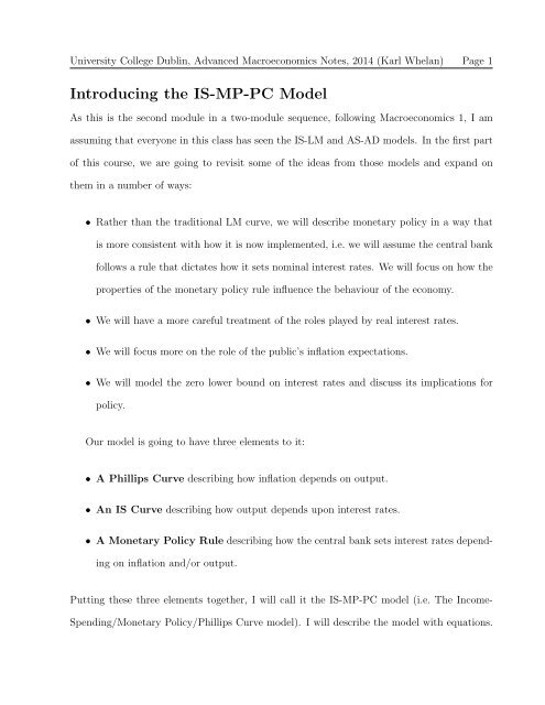
<strong>Introducing</strong> <strong>the</strong> <strong>IS</strong>-<strong>MP</strong>-<strong>PC</strong> <strong>Model</strong><br />
As this is <strong>the</strong> second module in a two-module sequence, following Macroeconomics 1, I am<br />
assuming that everyone in this class has seen <strong>the</strong> <strong>IS</strong>-LM and AS-AD models. In <strong>the</strong> first part<br />
of this course, we are going to revisit some of <strong>the</strong> ideas from those models and expand on<br />
<strong>the</strong>m in a number of ways:<br />
• Ra<strong>the</strong>r than <strong>the</strong> traditional LM curve, we will describe monetary policy in a way that<br />
is more consistent with how it is now implemented, i.e. we will assume <strong>the</strong> central bank<br />
follows a rule that dictates how it sets nominal interest rates. We will focus on how <strong>the</strong><br />
properties of <strong>the</strong> monetary policy rule influence <strong>the</strong> behaviour of <strong>the</strong> economy.<br />
• We will have a more careful treatment of <strong>the</strong> roles played by real interest rates.<br />
• We will focus more on <strong>the</strong> role of <strong>the</strong> public’s inflation expectations.<br />
• We will model <strong>the</strong> zero lower bound on interest rates and discuss its implications for<br />
policy.<br />
Our model is going to have three elements to it:<br />
• A Phillips Curve describing how inflation depends on output.<br />
• An <strong>IS</strong> Curve describing how output depends upon interest rates.<br />
• A Monetary Policy Rule describing how <strong>the</strong> central bank sets interest rates depending<br />
on inflation and/or output.<br />
Putting <strong>the</strong>se three elements toge<strong>the</strong>r, I will call it <strong>the</strong> <strong>IS</strong>-<strong>MP</strong>-<strong>PC</strong> model (i.e. The Income-<br />
Spending/Monetary Policy/Phillips Curve model). I will describe <strong>the</strong> model with equations.
University College Dublin, Advanced Macroeconomics Notes, 2014 (<strong>Karl</strong> <strong>Whelan</strong>) Page 2<br />
I will also merge toge<strong>the</strong>r <strong>the</strong> second two elements (<strong>the</strong> <strong>IS</strong> curve and <strong>the</strong> monetary policy<br />
rule) to give a new <strong>IS</strong>-<strong>MP</strong> curve that can be combined with <strong>the</strong> Phillips curve to use graphs<br />
to illustrate <strong>the</strong> model’s properties. 1<br />
<strong>Model</strong> Element One: The Phillips Curve<br />
Perhaps <strong>the</strong> most common <strong>the</strong>me in economics is that you can’t have everything you want. Life<br />
is full of trade-offs, so that if you get more of one thing, you have to have less of ano<strong>the</strong>r thing.<br />
In macroeconomics, <strong>the</strong>re are important trade-offs facing governments when <strong>the</strong>y implement<br />
policy. One of <strong>the</strong>se relates to a trade-off between desired outcomes for inflation and output.<br />
What form does this relationship take Back when macroeconomics was a relatively young<br />
discipline, in 1958, a study by <strong>the</strong> LSE’s A.W. Phillips seemed to provide <strong>the</strong> answer. Phillips<br />
documented a strong negative relationship between wage inflation and unemployment: Low<br />
unemployment was associated with high inflation, presumably because tight labour markets<br />
stimulated wage inflation. Figure 1 shows one of <strong>the</strong> graphs from Phillips’s paper illustrating<br />
<strong>the</strong> kind of relationship he found.<br />
In 1960, a paper by MIT economists Robert Solow and Paul Samuelson (both of whom<br />
would go on to win <strong>the</strong> Nobel prize in economics for o<strong>the</strong>r work) replicated <strong>the</strong>se findings<br />
for <strong>the</strong> US and emphasised that <strong>the</strong> relationship also worked for price inflation. Figure 2<br />
reproduces <strong>the</strong> graph in <strong>the</strong>ir paper describing <strong>the</strong> relationship <strong>the</strong>y found. The Phillips curve<br />
1 Though <strong>the</strong> particular model that will be presented in <strong>the</strong>se lectures can’t be found in any specific article<br />
or book, models that are very similar have been presented by a number of economists. In particular, <strong>the</strong><br />
article linked to on <strong>the</strong> website by Walsh (2002) presents a similar model. I have provided a links to Walsh’s<br />
paper on <strong>the</strong> website but only for those interested in seeing a versions of our model that consider some more<br />
advanced issues such as optimal monetary policy rules.
University College Dublin, Advanced Macroeconomics Notes, 2014 (<strong>Karl</strong> <strong>Whelan</strong>) Page 3<br />
quickly became <strong>the</strong> basis for <strong>the</strong> discussion of macroeconomic policy decisions. Economists<br />
advised that governments faced a tradeoff: Lower unemployment could be achieved, but only<br />
at <strong>the</strong> cost of higher inflation.<br />
However, Milton Friedman’s 1968 presidential address to <strong>the</strong> American Economic Association<br />
produced a well-timed and influential critique of <strong>the</strong> thinking underlying <strong>the</strong> Phillips<br />
curve. Friedman pointed out that it was expected real wages that affected wage bargaining.<br />
If low unemployment means workers have a strong bargaining position, <strong>the</strong>n high nominal<br />
wage inflation on its own is not good enough: They want nominal wage inflation greater than<br />
price inflation.<br />
Friedman argued that if policy-makers tried to exploit an apparent Phillips curve tradeoff,<br />
<strong>the</strong>n <strong>the</strong> public would get used to high inflation and come to expect it. Inflation expectations<br />
would move up and <strong>the</strong> previously-existing tradeoff between inflation and output would disappear.<br />
In particular, he put forward <strong>the</strong> idea that <strong>the</strong>re was a “natural” rate of unemployment<br />
and that attempts to keep unemployment below this level could not work in <strong>the</strong> long run.<br />
Evidence on <strong>the</strong> Phillips Curve<br />
Monetary and fiscal policies in <strong>the</strong> 1960s were very expansionary around <strong>the</strong> world, partly<br />
because governments following Phillips curve “recipes” chose booming economies with low<br />
unemployment at <strong>the</strong> expense of somewhat higher inflation.<br />
At first, <strong>the</strong> Phillips curve seemed to work: Inflation rose and unemployment fell. However,<br />
as <strong>the</strong> public got used to high inflation, <strong>the</strong> Phillips tradeoff got worse. By <strong>the</strong> late 1960s<br />
inflation was rising even though unemployment had moved up. Figure 3 shows <strong>the</strong> US time<br />
series for inflation and unemployment. This stagflation combination of high inflation and high
University College Dublin, Advanced Macroeconomics Notes, 2014 (<strong>Karl</strong> <strong>Whelan</strong>) Page 4<br />
unemployment got even worse in <strong>the</strong> 1970s. This was exactly what Friedman had predicted.<br />
Today, <strong>the</strong> data no longer show any sign of a negative relationship between inflation and<br />
unemployment. If fact, if you look at <strong>the</strong> scatter plot of US inflation and unemployment data<br />
shown in Figure 4, <strong>the</strong> correlation is positive: The original formulation of <strong>the</strong> Phillips curve<br />
is widely agreed to be wrong.
University College Dublin, Advanced Macroeconomics Notes, 2014 (<strong>Karl</strong> <strong>Whelan</strong>) Page 5<br />
Figure 1: A. W. Phillips’s Graph
University College Dublin, Advanced Macroeconomics Notes, 2014 (<strong>Karl</strong> <strong>Whelan</strong>) Page 6<br />
Figure 2: Solow and Samuelson’s Description of <strong>the</strong> Phillips Curve
University College Dublin, Advanced Macroeconomics Notes, 2014 (<strong>Karl</strong> <strong>Whelan</strong>) Page 7<br />
Figure 3: The Evolution of US Inflation and Unemployment<br />
12<br />
US Inflation and Unemployment, 1955-2013<br />
10<br />
8<br />
6<br />
4<br />
2<br />
0<br />
1955 1960 1965 1970 1975 1980 1985 1990 1995 2000 2005 2010<br />
Inflation<br />
Unemployment
University College Dublin, Advanced Macroeconomics Notes, 2014 (<strong>Karl</strong> <strong>Whelan</strong>) Page 8<br />
Figure 4: The Failure of <strong>the</strong> Original Phillips Curve<br />
11<br />
US Inflation and Unemployment, 1955-2013<br />
Inflation is <strong>the</strong> Four-Quarter Percentage Change in GDP Deflator<br />
10<br />
9<br />
Unemployment<br />
8<br />
7<br />
6<br />
5<br />
4<br />
3<br />
0 2 4 6 8 10 12<br />
Inflation
University College Dublin, Advanced Macroeconomics Notes, 2014 (<strong>Karl</strong> <strong>Whelan</strong>) Page 9<br />
Equations: Variables, Parameters and All That<br />
We will use both graphs and equations to describe <strong>the</strong> models in this class. Now I know many<br />
students don’t like equations and believe <strong>the</strong>y are best studiously avoided. However, that<br />
won’t be a good strategy for doing well in this course, so I strongly encourage you to engage<br />
with <strong>the</strong> technical material in this class. It isn’t as hard is it might look to start with.<br />
Variables and Coefficients: The equations in this class will generally have a certain format.<br />
They will often look a bit like this.<br />
y t = α + βx t (1)<br />
There are two types of objects in this equation. First, <strong>the</strong>re are <strong>the</strong> variables, y t and x t .<br />
These will correspond to economic variables that we are interested in (inflation or GDP for<br />
example). We interpret y t as meaning “<strong>the</strong> value that <strong>the</strong> variable y takes during <strong>the</strong> time<br />
period t”). For most models in this course, we will treat time as marching forward in discrete<br />
intervals, i.e. period 1 is followed by period 2, period t is followed by period t + 1 and so on.<br />
Second, <strong>the</strong>re are <strong>the</strong> parameters or coefficients. In this example, <strong>the</strong>se are given by α and<br />
β. These are assumed to stay fixed over time. There are usually two types of coefficients:<br />
Intercept terms like α that describe <strong>the</strong> value that series like y t will take when o<strong>the</strong>r variables<br />
all equal zero and coefficients like β that describe <strong>the</strong> impact that one variable has on ano<strong>the</strong>r.<br />
In this case, if β is a big number, <strong>the</strong>n a change in <strong>the</strong> variable x t has a big impact on y t while<br />
if β is small, it will have a small impact.<br />
Some of you are probably asking what those squiggly shapes — α and β — are. They<br />
are Greek letters. While it’s not strictly necessary to use <strong>the</strong>se shapes to represent model<br />
parameters, it’s pretty common in economics. So let me introduce <strong>the</strong>m: α is alpha (Al-Fa),<br />
β is beta (Bay-ta), γ is gamma, δ is delta, θ is <strong>the</strong>ta (Thay-ta) and π naturally enough is pi.
University College Dublin, Advanced Macroeconomics Notes, 2014 (<strong>Karl</strong> <strong>Whelan</strong>) Page 10<br />
Dynamics: One of <strong>the</strong> things we will be interested in is how <strong>the</strong> variables we are looking at<br />
will change over time. For example, we will have equations along <strong>the</strong> lines of<br />
y t = βy t−1 + γx t (2)<br />
Reading this equation, it says that <strong>the</strong> value of y at time t will depend on <strong>the</strong> value of x at<br />
time t and also on <strong>the</strong> value that y took in <strong>the</strong> previous period i.e. t − 1. By this, we mean<br />
that this equation holds in every period. In o<strong>the</strong>r words, in period 2, y depends on <strong>the</strong> value<br />
that x takes in period 2 and also on <strong>the</strong> value that y took in period 1. Similarly, in period 3,<br />
y depends on <strong>the</strong> value that x takes in period 3 and also on <strong>the</strong> value that y took in period<br />
2. And so on.<br />
Subscripts and Superscripts: When we write y t , we mean <strong>the</strong> value that <strong>the</strong> variable y takes<br />
at time t. Note that <strong>the</strong> t here is a subscript – it goes at <strong>the</strong> bottom of <strong>the</strong> y. Some students<br />
don’t realise this is a subscript and will just write yt but this is incorrect (it reads as though<br />
<strong>the</strong> value t is multiplying y which is not what’s going on).<br />
We will also sometimes put indicators above certain variables to indicate that <strong>the</strong>y are<br />
special variables. For example, in <strong>the</strong> model we present now, you will see a variable written<br />
as πt e which will represent <strong>the</strong> public’s expectation of inflation. In <strong>the</strong> model, π t is inflation at<br />
time t and <strong>the</strong> e above <strong>the</strong> π in πt e is <strong>the</strong>re to signify that this is not inflation itself but ra<strong>the</strong>r<br />
it is <strong>the</strong> public’s expectation of it.
University College Dublin, Advanced Macroeconomics Notes, 2014 (<strong>Karl</strong> <strong>Whelan</strong>) Page 11<br />
Our Version of <strong>the</strong> Phillips Curve<br />
We will use both graphs and equations to describe <strong>the</strong> various elements of our model. Our first<br />
element is an expectations-augmented Phillips curve which we will formulate as a relationship<br />
in which inflation depends on inflation expectations, <strong>the</strong> gap between output and its “natural”<br />
level and a temporary inflationary shock. Our equation for this is <strong>the</strong> following:<br />
π t = π e t + γ (y t − y ∗ t ) + ɛ π t (3)<br />
In this equation π represents inflation and by π t we mean inflation at time t. The equation<br />
states that inflation at time t depends on three factors:<br />
1. Inflation Expectations, π e t : This term—which puts an e superscript above <strong>the</strong> π t —<br />
represents <strong>the</strong> public’s inflation expectations at time t. We have put a time subscript<br />
on this variable because <strong>the</strong> public’s expectations may change over time.<br />
Note that<br />
a 1 point increase in inflation expectations raises inflation by exactly 1 point.<br />
This<br />
is because we are assuming that people bargain over real wages and higher expected<br />
inflation translates one-for-one into <strong>the</strong>ir wage bargaining, which in turn is passed into<br />
price inflation.<br />
2. The Output Gap, (y t − yt ∗ ): This is <strong>the</strong> gap between GDP at time t, as represented<br />
by y t , and what we will term <strong>the</strong> “natural” level of output, which we term yt ∗ . This<br />
is <strong>the</strong> level of output at time t that would be consistent with unemployment equalling<br />
its natural rate. (Note we are describing inflation as being dependent on <strong>the</strong> output<br />
gap ra<strong>the</strong>r than <strong>the</strong> gap between unemployment and its natural rate because this would<br />
require adding an extra element to <strong>the</strong> model, i.e. <strong>the</strong> link between unemployment and<br />
output). We would expect this natural level of output to gradually increase over time as
University College Dublin, Advanced Macroeconomics Notes, 2014 (<strong>Karl</strong> <strong>Whelan</strong>) Page 12<br />
productivity levels improve. The coefficient γ (pronounced “gamma”) describes exactly<br />
how much inflation is generated by a 1 percent increase in <strong>the</strong> gap between output and<br />
its natural rate.<br />
3. Temporary Inflationary Shocks, ɛ π t : No model in economics is perfect. So while<br />
inflation expectations and <strong>the</strong> output gap may be key drivers of inflation, <strong>the</strong>y won’t<br />
capture all <strong>the</strong> factors that influence inflation at any time. For example, “supply shocks”<br />
like a temporary increase in <strong>the</strong> price of imported oil can drive up inflation for a while.<br />
To capture <strong>the</strong>se kinds of temporary factors, we include an inflationary “shock” term,<br />
ɛ π t . (ɛ is a Greek letter pronounced “epsilon”). The superscript π indicates that this is<br />
<strong>the</strong> inflationary shock (this will distinguish it from <strong>the</strong> output shock that we will also<br />
add to <strong>the</strong> model) and <strong>the</strong> t subscript indicates that <strong>the</strong>se shocks change over time.<br />
The Phillips Curve Graph<br />
Figure 5 shows how to describe our Phillips curve equation in a graph. The graph shows a<br />
positive relationship between inflation and output. The key points to notice are <strong>the</strong> markings<br />
on <strong>the</strong> two axes indicating what happens when output is at its natural rate.<br />
This graph<br />
illustrates <strong>the</strong> case when <strong>the</strong>re are no temporary inflationary shocks so ɛ π t<br />
= 0. In this case,<br />
<strong>the</strong> Phillips curve is just<br />
π t = π e t + γ (y t − y ∗ t ) (4)<br />
So when y t = y ∗ t<br />
we get π t = π e t . This is a key aspect of this graph. If you are asked to draw<br />
this graph in <strong>the</strong> final exam and you just draw an upward-sloping curve without describing<br />
<strong>the</strong> key points on <strong>the</strong> inflation and output axes, you won’t score many points.<br />
The curve can move up or down depending on what happens to <strong>the</strong> inflationary shocks,
University College Dublin, Advanced Macroeconomics Notes, 2014 (<strong>Karl</strong> <strong>Whelan</strong>) Page 13<br />
ɛ π t , and with inflation expectations. Figure 6 illustrates what happens when <strong>the</strong>re is a positive<br />
inflationary shock so that ɛ π t<br />
goes from being zero to being positive. In this case, even when<br />
output equals its natural level (i.e. y t = y ∗ t ) we still get inflation being above its expected<br />
level. Figure 7 illustrates how <strong>the</strong> curve changes when expected inflation rises from π 1 to π 2 .<br />
The whole curve shifts upwards because of <strong>the</strong> increase in expected inflation.
University College Dublin, Advanced Macroeconomics Notes, 2014 (<strong>Karl</strong> <strong>Whelan</strong>) Page 14<br />
Figure 5: The Phillips Curve with ɛ π t = 0<br />
Inflation<br />
Output
University College Dublin, Advanced Macroeconomics Notes, 2014 (<strong>Karl</strong> <strong>Whelan</strong>) Page 15<br />
Figure 6: The Phillips Curve as we move from ɛ π t = 0 to ɛ π t > 0<br />
(An Aggregate Supply Shock)<br />
Inflation<br />
<strong>PC</strong> ( > 0)<br />
<strong>PC</strong> ( =0)<br />
Output
University College Dublin, Advanced Macroeconomics Notes, 2014 (<strong>Karl</strong> <strong>Whelan</strong>) Page 16<br />
Figure 7: The Phillips Curve as we move from π e t = π 1 to π e t = π 2<br />
Inflation<br />
<strong>PC</strong> ( )<br />
<strong>PC</strong> ( )<br />
Output
University College Dublin, Advanced Macroeconomics Notes, 2014 (<strong>Karl</strong> <strong>Whelan</strong>) Page 17<br />
<strong>Model</strong> Element Two: The <strong>IS</strong> Curve<br />
The second element of <strong>the</strong> model is one that should be familiar to you: An <strong>IS</strong> curve relating<br />
output to interest rates. The higher interest rates are, <strong>the</strong> lower output is. However, I want<br />
to stress something here that is often not emphasised in introductory treatments of <strong>the</strong> <strong>IS</strong><br />
curve. The <strong>IS</strong> relationship is between output and real interest rates, not nominal rates. Real<br />
interest rates adjust <strong>the</strong> headline (nominal) interest rate by subtracting off inflation.<br />
Think for a second about why it is that real interest rates are what matters. You know<br />
already that high interest rates discourage aggregate demand by reducing consumption and<br />
investment spending. But what is a high interest rate Suppose I told you <strong>the</strong> interest rate<br />
was 10 percent. Is this a high interest rate<br />
You might be inclined to say, “Yes, this is a high interest rate” but <strong>the</strong> answer is that it<br />
really depends on inflation. Consider <strong>the</strong> decision to save for tomorrow or spend today. The<br />
argument for saving is that it can allow you to consume more tomorrow. If <strong>the</strong> real interest<br />
rate is positive, <strong>the</strong>n this means that you will be able to purchase more goods and services<br />
tomorrow with <strong>the</strong> money that you set aside.<br />
For instance, if <strong>the</strong> interest rate if 5% but<br />
inflation is 2%, <strong>the</strong>n you’ll be able to buy 3% more stuff next year because you saved. In<br />
constrast, if <strong>the</strong> interest rate if 5% but inflation is 8%, <strong>the</strong>n you’ll be able to buy 3% less stuff<br />
next year even though you have saved your money and earned interest. For <strong>the</strong>se reasons, it<br />
is <strong>the</strong> real interest rate that determines whe<strong>the</strong>r consumers think saving is attractive relative<br />
to spending.<br />
The same logic applies to firms thinking about borrowing to make investment purchases.<br />
If inflation is 10%, <strong>the</strong>n a firm can expect that its prices (and profits) will be increasing by<br />
that much over <strong>the</strong> next year and a 10% interest rate won’t seem so high. But if prices are
University College Dublin, Advanced Macroeconomics Notes, 2014 (<strong>Karl</strong> <strong>Whelan</strong>) Page 18<br />
falling, <strong>the</strong>n a 10% interest rate on borrowings will seem very high.<br />
With <strong>the</strong>se ideas in mind, our version of <strong>the</strong> <strong>IS</strong> curve will be <strong>the</strong> following:<br />
y t = y ∗ t − α (i t − π t − r ∗ ) + ɛ y t (5)<br />
Expressed in words, this equation states that <strong>the</strong> gap between output and its natural rate<br />
(y t − y ∗ t ) depends on two factors:<br />
1. The Real Interest Rate: The nominal interest rate at time t is represented by i t ,<br />
so <strong>the</strong> real interest rate is i t − π t . The coefficient α (pronounced “alpha”) describes<br />
<strong>the</strong> effect of a one point increase in <strong>the</strong> real interest rate on output. The equation has<br />
been constructed in a particular way so that it explicitly defines <strong>the</strong> real interest rate<br />
at which output will, on average, equal its natural rate. This rate can be termed <strong>the</strong><br />
“‘natural rate of interest” a term first used by early 20th century Swedish economist<br />
Knut Wicksell. Specifically, we can see from <strong>the</strong> equation that if ɛ y t<br />
= 0 <strong>the</strong>n a real<br />
interest rate of r ∗ will imply y t = y ∗ t .<br />
2. Aggregate Demand Shocks, ɛ y t : The <strong>IS</strong> curve is an even more threadbare model of<br />
output than <strong>the</strong> Phillips curve model is of inflation. Many o<strong>the</strong>r factors beyond <strong>the</strong><br />
real interest rate influence aggregate spending decisions.<br />
These include fiscal policy,<br />
asset prices and consumer and business sentiment. We will model all of <strong>the</strong>se factors<br />
as temporary deviations from zero of an aggregate demand “shock”, ɛ y t . Note that this<br />
shock has a superscript y to distinguish it from <strong>the</strong> “aggregate supply” shock ɛ π t<br />
that<br />
moves <strong>the</strong> Phillips curve up and down.
University College Dublin, Advanced Macroeconomics Notes, 2014 (<strong>Karl</strong> <strong>Whelan</strong>) Page 19<br />
<strong>Model</strong> Element Three: A Monetary Policy Rule<br />
Thus far, our model has described how inflation depends on output and how output depends<br />
on interest rates. We can complete <strong>the</strong> model by describing how interest rates are determined.<br />
Traditionally, in <strong>the</strong> <strong>IS</strong>-LM model, this is where <strong>the</strong> LM curve is introduced. The LM<br />
curve links <strong>the</strong> demand for <strong>the</strong> real money stock with nominal interest rates and output, with<br />
a relationship of <strong>the</strong> form<br />
m t<br />
p t<br />
= δ − µi t + θy t (6)<br />
For a given stock of money (m t ) and a given level of prices (p t ), this relationship can be<br />
re-arranged to give a positive relationship between output and interest rates of <strong>the</strong> form<br />
y t = 1 θ<br />
(<br />
mt<br />
p t<br />
− δ + µi t<br />
)<br />
(7)<br />
This positive relationship between output and interest rates is combined with <strong>the</strong> negative<br />
relationship between <strong>the</strong>se variables in <strong>the</strong> <strong>IS</strong> curve to determine unique values for output and<br />
interest rates, something that can be illustrated in a graph with an upward-sloping LM curve<br />
and a downward-sloping <strong>IS</strong> curve. Monetary policy is <strong>the</strong>n described as taking <strong>the</strong> form of<br />
<strong>the</strong> central bank adjusting <strong>the</strong> money supply m t in a way that sets <strong>the</strong> position of <strong>the</strong> LM<br />
curve. The determination of prices is usually described separately in an AS-AD model.<br />
We will not be using <strong>the</strong> LM curve, for three reasons.<br />
1. Realism 1: In practice, no modern central bank implements its monetary policy by<br />
setting a specified level of <strong>the</strong> monetary base. Instead, <strong>the</strong>y use <strong>the</strong>ir power to supply<br />
potentially unlimited amounts of liquidity to set short-term interest rates to equal a<br />
target level. The supply of base money ends up being whatever emerges from enforcing<br />
<strong>the</strong> interest rate target. This approach — which has been <strong>the</strong> practice at all <strong>the</strong> major
University College Dublin, Advanced Macroeconomics Notes, 2014 (<strong>Karl</strong> <strong>Whelan</strong>) Page 20<br />
central banks for at least 30 years — makes <strong>the</strong> LM curve (and <strong>the</strong> money supply) of<br />
secondary interest when thinking about core macroeconomic issues. Our approach will<br />
be to describe how <strong>the</strong> central bank sets interest rates and we won’t focus on <strong>the</strong> money<br />
supply.<br />
2. Realism 2: The traditional approach is for <strong>IS</strong>-LM to describe <strong>the</strong> determination of<br />
output and interest rates. Then a separate AS-AD model is used to describe <strong>the</strong> determination<br />
of prices (and thus, implicitly, inflation). However, <strong>the</strong> reality is that ra<strong>the</strong>r<br />
than being determined independently of inflation, most modern central banks set interest<br />
rates with a very close eye on inflationary developments. A model that integrates<br />
<strong>the</strong> determination of inflation with <strong>the</strong> setting of monetary policy is thus more realistic.<br />
3. Simplicity: In simplifying <strong>the</strong> determination of output, inflation and interest rates<br />
down to a single model, this approach is also simpler than one that requires two different<br />
sets of graphs.<br />
We will consider two different types of monetary policy rules that may be followed by <strong>the</strong><br />
central bank in our model. The first one is a simple one in which <strong>the</strong> central bank adjusts its<br />
interest rate in line with inflation with <strong>the</strong> goal of meeting an inflation target. Specifically,<br />
<strong>the</strong> first rule we will consider is <strong>the</strong> following one:<br />
i t = r ∗ + π ∗ + β π (π t − π ∗ ) (8)<br />
In English, <strong>the</strong> rule can be intepreted as follows: The central bank adjusts <strong>the</strong> nominal interest<br />
rate, i t , upwards when inflation, π t , goes up and downwards when inflation goes down (we<br />
are assuming that β π > 0) and it does so in a way that means when inflation equals a target<br />
level, π ∗ , chosen by <strong>the</strong> central bank, real interest rates will be equal to <strong>the</strong>ir natural level.
University College Dublin, Advanced Macroeconomics Notes, 2014 (<strong>Karl</strong> <strong>Whelan</strong>) Page 21<br />
That’s a bit of a mouthful, so let’s see that this is <strong>the</strong> case and <strong>the</strong>n try to understand<br />
why <strong>the</strong> monetary policy rule would take this form. First, note what <strong>the</strong> nominal interest<br />
rate will be if inflation equals its target level (i.e. π t = π ∗ ). The term after <strong>the</strong> final plus sign<br />
in equation (8) will equal zero and <strong>the</strong> nominal interest rate will be<br />
i t = r ∗ + π ∗ (9)<br />
In this case, because π t = π ∗ , we can also write this as<br />
i t = r ∗ + π t (10)<br />
So <strong>the</strong> real interest rate will be<br />
i t − π t = r ∗ (11)<br />
Now think about why a rule of this form might be a good idea. Suppose <strong>the</strong> central bank<br />
has a target inflation rate of π ∗ that it wants to achieve. Ideally, it would like <strong>the</strong> public to<br />
understand that this is <strong>the</strong> likely inflation rate that will occur, so that πt e = π ∗ . If that can<br />
be achieved, <strong>the</strong>n <strong>the</strong> Phillips curve (equation 3) tells us that, on average, inflation will equal<br />
π ∗ provided we have y t = yt ∗ . And <strong>the</strong> <strong>IS</strong> curve tells us that, on average, we will have y t = yt<br />
∗<br />
when i t − π t = r ∗ . So this is a policy that can help to enforce an average inflation rate equal<br />
to <strong>the</strong> central bank’s desired target, provided <strong>the</strong> public adjusts its inflationary expectations<br />
accordingly.
University College Dublin, Advanced Macroeconomics Notes, 2014 (<strong>Karl</strong> <strong>Whelan</strong>) Page 22<br />
The <strong>IS</strong>-<strong>MP</strong> Curve<br />
That’s <strong>the</strong> model. It consists of three equations. Let’s pull <strong>the</strong>m toge<strong>the</strong>r in one place. They<br />
are <strong>the</strong> Phillips curve:<br />
π t = πt e + γ (y t − yt ∗ ) + ɛ π t (12)<br />
The <strong>IS</strong> curve:<br />
y t = yt ∗ − α (i t − π t − r ∗ ) + ɛ y t (13)<br />
And <strong>the</strong> monetary policy rule:<br />
i t = r ∗ + π ∗ + β π (π t − π ∗ ) (14)<br />
Now you may recall that I had promised a graphical representation of this model. However,<br />
this is a system of three variables which makes it hard to express on a graph with two axes.<br />
To make <strong>the</strong> model easier to analyse using graphs, we are going to reduce it down to a system<br />
with two main variables (inflation and output). We can do this because <strong>the</strong> monetary policy<br />
rule makes interest rates are a function of inflation, so we can substitute this rule into <strong>the</strong><br />
<strong>IS</strong> curve to get a new relationship between output and inflation that we will call <strong>the</strong> <strong>IS</strong>-<strong>MP</strong><br />
curve.<br />
We do this as follows. Replace <strong>the</strong> term i t in equation (13) with <strong>the</strong> right-hand-side of<br />
equation (14) to get<br />
y t = y ∗ t − α [r ∗ + π ∗ + β π (π t − π ∗ )] + α (π t + r ∗ ) + ɛ y t (15)<br />
Now multiply out <strong>the</strong> terms in this equation to get<br />
y t = y ∗ t − αr ∗ − απ ∗ − αβ π (π t − π ∗ ) + απ t + αr ∗ + ɛ y t (16)
University College Dublin, Advanced Macroeconomics Notes, 2014 (<strong>Karl</strong> <strong>Whelan</strong>) Page 23<br />
We can bring toge<strong>the</strong>r <strong>the</strong> two terms being multiplied by α on its own, and cancel out <strong>the</strong><br />
term terms in αr ∗ to get<br />
y t = y ∗ t − αβ π (π t − π ∗ ) + α (π t − π ∗ ) + ɛ y t (17)<br />
which simplifies to<br />
y t = yt ∗ − α (β π − 1) (π t − π ∗ ) + ɛ y t (18)<br />
This is <strong>the</strong> <strong>IS</strong>-<strong>MP</strong> curve. It combines <strong>the</strong> information in <strong>the</strong> <strong>IS</strong> curve and <strong>the</strong> <strong>MP</strong> curve into<br />
one relationship.<br />
The <strong>IS</strong>-<strong>MP</strong> Curve Graph<br />
What would this curve look like on a graph It turns out it depends especially on <strong>the</strong> value of<br />
β π , <strong>the</strong> parameter that describes how <strong>the</strong> central bank reacts to inflation. The <strong>IS</strong>-<strong>MP</strong> curve<br />
says that an extra unit of inflation implies a change of −α (β π − 1) in output. Is this positive<br />
or negative Well we are assuming that α > 0 (we put a negative sign in front of this when<br />
determining <strong>the</strong> effect of real interest rates on output) so this combined coefficient will be<br />
negative if β π − 1 > 0.<br />
In o<strong>the</strong>r words, <strong>the</strong> <strong>IS</strong>-<strong>MP</strong> curve will have a negative slope (slope downwards) provided<br />
<strong>the</strong> central bank reacts to inflation so that β π > 1. The explanation for this is as follows.<br />
An increase in inflation of x will lead to an increase in nominal interest rates of β π x so real<br />
interest rates change by (β π − 1) x. This means that if β π > 1 an increase in inflation leads<br />
to higher real interest rates and, via <strong>the</strong> <strong>IS</strong> curve relation, to lower output. So if β π > 1<br />
<strong>the</strong>n <strong>the</strong> <strong>IS</strong>-<strong>MP</strong> curve can be depicted as a downward-sloping curve. In contrast, if β π < 1,<br />
<strong>the</strong>n an increase in inflation leads to lower real interest rates and higher output, implying an<br />
upward-sloping <strong>IS</strong>-<strong>MP</strong> curve.
University College Dublin, Advanced Macroeconomics Notes, 2014 (<strong>Karl</strong> <strong>Whelan</strong>) Page 24<br />
For now, we will assume that β π > 1 so that we have a downward-sloping <strong>IS</strong>-<strong>MP</strong> curve<br />
but we will revisit this issue after a few more lectures. Figure 8 thus shows what <strong>the</strong> <strong>IS</strong>-<strong>MP</strong><br />
curve looks like when <strong>the</strong> aggregate demand shock ɛ y t = 0. Again, <strong>the</strong> key thing to notice is<br />
<strong>the</strong> value of inflation that occurs when output equals its natural rate. When y t = y ∗ t<br />
we get<br />
π t = π ∗ . As with <strong>the</strong> Phillips curve, if you are asked to draw this graph in <strong>the</strong> final exam and<br />
you just draw an downward-sloping curve without describing <strong>the</strong> key points on <strong>the</strong> inflation<br />
and output axes, you won’t score many points.
University College Dublin, Advanced Macroeconomics Notes, 2014 (<strong>Karl</strong> <strong>Whelan</strong>) Page 25<br />
Figure 8: The <strong>IS</strong>-<strong>MP</strong> Curve with ɛ y t = 0<br />
Inflation<br />
Output
University College Dublin, Advanced Macroeconomics Notes, 2014 (<strong>Karl</strong> <strong>Whelan</strong>) Page 26<br />
Figure 9: The <strong>IS</strong>-<strong>MP</strong> curve as we move from ɛ y t = 0 to ɛ y t > 0<br />
(An Aggregate Demand Shock)<br />
Inflation<br />
<strong>IS</strong>-<strong>MP</strong> ( > 0)<br />
Output<br />
<strong>IS</strong>-<strong>MP</strong> ( =0)
University College Dublin, Advanced Macroeconomics Notes, 2014 (<strong>Karl</strong> <strong>Whelan</strong>) Page 27<br />
The Full <strong>Model</strong><br />
The full <strong>IS</strong>-<strong>MP</strong>-<strong>PC</strong> model can be illustrated in <strong>the</strong> traditional fashion as a graph with one<br />
curve that slopes upwards (<strong>the</strong> Phillips curve) and one that slopes downwards (<strong>the</strong> <strong>IS</strong>-<strong>MP</strong><br />
curve provided we assume that β π > 1.) Figure 10 provides <strong>the</strong> simplest possible example of<br />
<strong>the</strong> graph. This is <strong>the</strong> case where both <strong>the</strong> temporary shocks, ɛ π t and ɛ y t equal zero and <strong>the</strong><br />
public’s expectation of inflation is equal to <strong>the</strong> central bank’s inflation target. Note that I have<br />
labelled <strong>the</strong> <strong>PC</strong> and <strong>IS</strong>-<strong>MP</strong> curves to explicitly indicate what <strong>the</strong> expected and target rates<br />
of inflation are and it will be a good idea for you to do <strong>the</strong> same when answering questions<br />
about this model.<br />
In <strong>the</strong> next set of notes, we will analyse this model in depth, examining what happens<br />
when various types of events occur and focusing carefully on how inflation expectations change<br />
over time.
University College Dublin, Advanced Macroeconomics Notes, 2014 (<strong>Karl</strong> <strong>Whelan</strong>) Page 28<br />
Figure 10: The <strong>IS</strong>-<strong>MP</strong>-<strong>PC</strong> <strong>Model</strong> When Expected Inflation Equals<br />
<strong>the</strong> Inflation Target<br />
Inflation<br />
<strong>IS</strong>-<strong>MP</strong> (<br />
<strong>PC</strong> ( )<br />
Output
University College Dublin, Advanced Macroeconomics Notes, 2014 (<strong>Karl</strong> <strong>Whelan</strong>) Page 29<br />
A More Complicated Monetary Policy Rule: The Taylor Rule<br />
Before moving on to analyse <strong>the</strong> model in more depth, I want to describe <strong>the</strong> more complex<br />
version of <strong>the</strong> monetary policy rule that I alluded to earlier. This rule takes a form that is<br />
associated with Stanford economist John Taylor. In a famous paper published in 1993 called<br />
“Discretion Versus Policy Rules in Practice” (you will find a link on <strong>the</strong> class webpage) Taylor<br />
noted that Federal Reserve policy in <strong>the</strong> few years before his paper was published seemed to<br />
be characterised by a rule in which interest rates were adjusted in response to both inflation<br />
and <strong>the</strong> gap between output and an estimated trend.<br />
Within our model structure, we can amend our monetary policy rule to be more like this<br />
“Taylor rule” if we make it take <strong>the</strong> following form:<br />
i t = r ∗ + π ∗ + β π (π t − π ∗ ) + β y (y t − y ∗ t ) (19)<br />
It turns out that <strong>the</strong> properties of <strong>the</strong> <strong>IS</strong>-<strong>MP</strong>-<strong>PC</strong> model don’t really change if we adopt<br />
this more complicated monetary policy rule. If we substitute <strong>the</strong> expression for <strong>the</strong> nominal<br />
interest rate in (19) into <strong>the</strong> <strong>IS</strong> curve equation (5), we get<br />
y t = y ∗ t − α [r ∗ + π ∗ + β π (π t − π ∗ ) + β y (y t − y ∗ t )] + α (π t + r ∗ ) + ɛ y t (20)<br />
This can be re-arranged as follows (canceling out <strong>the</strong> terms involving r ∗ ):<br />
y t − y ∗ t = −αβ y (y t − y ∗ t ) − αβ π (π t − π ∗ ) − απ ∗ + απ t + ɛ y t (21)<br />
Bringing toge<strong>the</strong>r all <strong>the</strong> terms involving <strong>the</strong> output gap y t − y ∗ t , we get<br />
(1 + αβ y ) (y t − y ∗ t ) = −αβ π (π t − π ∗ ) + α (π t − π ∗ ) + ɛ y t (22)<br />
Which can be expressed as<br />
y t − yt ∗ = − α (β π − 1)<br />
(π t − π ∗ 1<br />
) + ɛ y t (23)<br />
1 + αβ y 1 + αβ y
University College Dublin, Advanced Macroeconomics Notes, 2014 (<strong>Karl</strong> <strong>Whelan</strong>) Page 30<br />
This equation shows us that broadening <strong>the</strong> monetary policy rule to incorporate interest rates<br />
responding to <strong>the</strong> output gap doesn’t change <strong>the</strong> essential form of <strong>the</strong> <strong>IS</strong>-<strong>MP</strong> curve. As long<br />
as β π > 1, <strong>the</strong> curve will slope downwards and will feature π t = π ∗ when y t = y ∗ t<br />
and <strong>the</strong>re<br />
are no inflationary shocks. So while <strong>the</strong> addition of an output gap response to <strong>the</strong> monetary<br />
policy rule changes <strong>the</strong> coefficients of <strong>the</strong> <strong>IS</strong>-<strong>MP</strong> model a bit, it doesn’t change <strong>the</strong> underlying<br />
economics. In <strong>the</strong> analysis in <strong>the</strong> next sets of notes, we will stick with <strong>the</strong> model that uses<br />
<strong>the</strong> basic “inflation targeting” monetary policy rule.<br />
Things to Understand from <strong>the</strong>se Notes<br />
Here’s a brief summary of <strong>the</strong> things that you need to understand from <strong>the</strong>se notes.<br />
1. The evidence on <strong>the</strong> Phillips curve.<br />
2. The Phillips curve that features in our model and how to draw it.<br />
3. Why real interest rates are what matters for aggregage demand.<br />
4. The <strong>IS</strong> curve that features in our model.<br />
5. The monetary policy that features in our model.<br />
6. How to derive <strong>the</strong> <strong>IS</strong>-<strong>MP</strong> curve.<br />
7. What determines <strong>the</strong> slope of <strong>the</strong> <strong>IS</strong>-<strong>MP</strong> curve.<br />
8. How <strong>the</strong> <strong>IS</strong>-<strong>MP</strong> curve changes when <strong>the</strong> monetary policy rule takes <strong>the</strong> form of a “Taylor<br />
rule”.