Estimation of Zero Coupon Curves in DataMetrics

Estimation of zero-coupon curves in 

DataMetrics 

Allan Malz 

RiskMetrics Group 

allan.malz@riskmetrics.com 

DataMetrics is modifying its technique for estimating zero-coupon interbank and government 

benchmark curves. The new algorithm is employed together with additional 

synchronized input data to deliver better-quality curves. The modified technique assumes 

the instantaneous forward rate is a constant between the maturity dates of observable 

interest rates. Together, the flat forward technique and new input data increase pricing 

and risk measurement accuracy, particularly at the short end. The flat forward technique 

is shown to be preferable to plausible alternative approaches. 

DataMetrics is modifying the bootstrapping technique it uses to estimate zero-coupon curves. 

The modified bootstrapping technique assumes the instantaneous forward interest rate is a 

constant between observed bond or other security maturities. We therefore refer to it as 

the “flat forward” technique. DataMetrics applies it to a range of interbank and government 

benchmark zero-coupon curves in both key currencies and emerging markets. 

The new algorithm is being employed together with additional input data to deliver better-quality 

curves. Together, the flat forward technique and new input data provide several advantages: 

• The underlying data for the interbank and government curves, particularly the government 

bonds, can be sparse. For example, there are only 6 U.S. Treasury benchmarks, of which 

3 are T-bills and 3 are coupon bonds. The flat forward approach avoids potentially adding 

spurious information to that contained in the modest available underlying data set, while 

still permitting accurate pricing. 

• It permits DataMetrics to estimate time series of spot interest rates with any time to 

maturity ranging from overnight to 30 years, applying any desired compounding interval 

or day count convention uniformly across the curve. In particular, it becomes it easy to 

add new RiskMetrics vertexes if needed and supported by the data. It also permits the 

generation of time series of forward rates with any compounding interval, time to maturity, 

or time to settlement. 

• It increases the pricing accuracy of DataMetrics fixed-income curves for fixed-income instruments, 

particularly at the short end. 

• The new approach improves the accuracy of volatility and correlation estimates and thus of 

fixed-income risk measures generally. It particularly enhances risk reporting for short-term 

fixed income positions and for money-market futures spread trades. 

• The modified bootstrapping technique permits the original security prices used in the estimation 

procedure to be recovered from spot rates. For example, if a money market futures

RiskMetrics Journal, Volume 3(1) 28 

expiring in exactly 15 months is used in the procedure, the implied rate can be recovered 

from the estimated 15- and 18-month spot rates. 

• The data underlying the curves can generally be captured simultaneously, so the new curves 

will be synchronous. 

We can think of an interest-rate curve as an unobservable price schedule for fixed income 

securities with the same liquidity and credit-risk characteristics, but diverse cash flow structures 

and day count and compounding conventions. A government benchmark curve is the price 

schedule for central government obligations; an interbank curve is the price schedule for debt 

between highly-rate banks, or between banks and highly-rated corporate counterparties. Such 

price schedules should be expected to accurately reflect interest rates on any fixed-income 

security in that category, regardless of cash flow structure and day count and compounding 

conventions. 

The flat forward approach fully exploits all the information about an interest rate curve contained 

in the observable market data, while at the same time adding no additional assumptions about 

the level and shape of the curve. The precise settlement practices, maturity dates, compounding 

frequency, pay frequency and day count conventions underlying the input data are taken into 

account in the calculations. 1 

1 Constructing the curve: source data 

There are two aspects to the curve construction technique: how the raw data are manipulated, 

and how the raw data are selected from the many fixed-income securities on the curve. We 

will take them in turn in this and the next section. 

Interbank or swap curves represent interest rates on unsecured, non-negotiable loans between 

high-quality banks and corporations. They can be based on interbank deposit rates or fixings, 

money market futures, and plain vanilla swap rates. The shortest maturity points on the 

interbank curve are generally derived from indicative deposit rates or deposit rate fixings. 

Where available, the first point on the curve is an overnight rate, generally an overnight Libor 

or repo rate. For the U.S. dollar (effective Fed funds) and the Euro (Eonia), a weighted 

average index of overnight transactions are available. For emerging market currencies and 

some industrial country currencies, overnight index swap rates and money market rates implied 

by foreign exchange forwards may be used. Where available, money market futures are used 

for the 3-month to 2- or 3-year sector, and swap rates for the longer-term sector. 

Government benchmark curves represent default risk-free interest rates. Central or federal 

government bills and bonds are used where possible. In some cases, liquid markets in shortterm 

central government debt do not exist. In that case, interbank obligations may be used to 

construct the short end of the curve. 

1 Further detail on the flat forward technique is contained in Malz (2002). Earlier work on DataMetrics yield curves 

is presented in Zangari (1997). Fabozzi (1999) has a textbook description of the standard bootstrapping approach to 

yield curve estimation. A recent example of the use of the flat forward technique, by the European Central Bank, is 

described in Brousseau (2002).

29 Estimation of zero-coupon curves in DataMetrics 

Table 1 

Interbank curve data sources by maturity range 

U.S. dollar 

Overnight Effective Federal funds rate or USD deposits Actual/360 

1 week to 3 months USD deposits Actual/360 

3 months to 2 years Settlement prices of Chicago Mercantile Exchange Actual/360 

(CME) 3-month Eurodollar futures 

2 years to 30 years Plain vanilla interest rate swaps vs. 6-month Libor Semiannual bond basis 

flat 

Euro 

Overnight EONIA or EUR deposits Actual/360 

1 week to 3 months EUR deposits Actual/360 

3 months to 2 years Settlement prices of London International Financial Actual/360 

Futures and Options Exchange (LIFFE) 3-month Euribor 

futures 

2 years to 30 years Plain vanilla interest rate swaps vs. 6-month Libor 

flat 

Annual bond basis 

The source data generally has different day count conventions. All rates are converted if 

necessary to a common day count convention of Actual/365 as part of the curve estimation 

procedure. For money market rates and rates implied by 3-month money market futures, 

this generally involves multiplying the rates by 360 . Futures on 3-month money market rates 

365 

are treated as having a time to maturity of exactly 91 years. Regardless of the day count 

365 

basis or other bond-mathematical conventions underlying the input data, the output data can 

be converted to any desired basis. DataMetrics and RiskManager employ Actual/365 as a 

common default day count basis for all curves. 

In many cases, settlement of fixed-income transactions occurs one or several days after the 

counterparties conclude a deal. For example, the value date for most OTC money market 

transactions is 2 days after the transaction date. We take the time to settlement into account 

in identifying the maturity date correctly for money market transactions less than 1 year. 

However, we do not take the time to settlement itself into account in setting discount factors 

and zero-coupon rates for two reasons. First, in most cases, the time to settlement is not 

uniform across the data sources underlying the curves. Second, and more importantly, the time 

to settlement does not affect the validity of the interest rate as a representation of today’s 

price of money for the term to maturity, as interest is not charged until the value date. 

Details are presented in Table 1 for the USD and EUR interbank curves. 

2 Constructing the curve: mechanics 

Each curve has a short-maturity segment based on add-on or discount rates or forwards or 

futures on add-on or discount rates. This sector of the curve, called the “stub,” does not 

require bootstrapping, as the rates on the underlying instruments can be readily converted to


zero-coupon or spot rates. Longer term rates are based on coupon bonds or swaps. The 

longer-term portion of each curve is bootstrapped using the flat forward assumption. The 

precise settlement practices, maturity dates, compounding frequency, pay frequency and day 

count conventions underlying the input data are taken into account in the calculations. 

2.1 Notation 

We let t denote the current date, T and its subscripted variants a maturity, settlement or payment 

date, and τ and its subscripted variants, measured in years, a time to maturity, settlement or 

payment. 

The immediate output of the procedure is a set of instantaneous forward rates with specific 

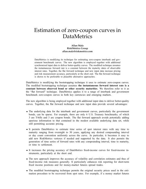
settlement dates, which we call forward vertexes, as shown in Figure 1. Let T j ,j = 0, 1, ..., N 

be the forward vertexes for which instantaneous forward rates are estimated, and let {f τj } N j=1 

be the set of estimated instantaneous forward rates from which the curve is constructed. The 

indexing is carried out so that each instantaneous forward rate f τj applies on the interval 

[τ j−1 ,τ j ). The flat forward assumption implies that for any 0 ≤ τ ≤ τ N ,f τ = f min[{τj |τ j >τ}]. 

As a convention, we set τ 0 ≡ 0; for τ ≥ τ N ,wesetf τ = f τN . 

2.2 Relationships among spot and forward rates 

A τ-year continuously compounded spot rate, that is, the constant annual rate at which a 

pure discount bond’s value must grow to reach one currency unit at time T , is computed by 

integrating the instantaneous forward curve over the time to maturity: 

r τ = 1 τ 

∫ τ 

0 

f s ds. (1) 

If the instantaneous forward rate is higher (lower) than the spot rate for maturity τ, the spot 

rate rises (falls) at the exponential rate 1 τ (f τ − r τ ), as shown in Figure 1. 

Discount factors, that is, the time-t prices of pure discount bonds maturing at time T are 

constructed from the forward rates or spot rates. The discount factor p τ is related to spot 

rates by 

( ∫ τ 

) 

p τ = e −r τ τ = exp − f s ds . (2) 

0 

2.3 Constructing the stub portion 

Deposit rates are expressed as annual add-on rates, that is, interest is computed by multiplying 

the quoted rate by the fraction of a year for which interest will be applied. Let r dep 

t,T 

represent 

a τ ≡ T − t deposit rate. Its discrete compounding interval is equal to t − T = τ. The time 

to maturity of a deposit or fixing is computed from the actual maturity date, which in turn


Figure 1 

Forward and spot rates 

3.30 

forward 

spot 

3.25 

1 7 30 60 

Instantaneous forward rates and continuously compounded spot rates, EUR 

swap curve, Nov. 16, 2001. 

is computed using the ISDA Modified Following Business Day convention and its refinements 

for maturities below 1 month. 

The continuously compounded spot rate r t,T 

is 

r t,T = 

ln(1 + r 

dep 

τ 

t,T τ) 

. (3) 

A continuously compounded forward rate f t,T1 ,T 2 

with time to settlement τ 1 and time to maturity 

τ 2 can be computed from the continuously compounded spot rates derived from two deposit 

rates with maturities T 1 and T 2 . Letting T 1 − t = τ 1 and T 2 − T 1 = τ 2 , 

f t,T1 ,T 2 

= r t,T 2 

(τ 1 + τ 2 ) + r t,T1 τ 1 

τ 2 

. (4) 

We need next to convert the forward with a discrete time to maturity (τ 2 ) to an instantaneous 

forward curve. A forward rate with a discrete time to maturity is the average of the instantaneous 

forward rates over the time to maturity: 

f t,T1 ,T 2 

= 1 τ 2 

∫ T2 

T 1 

f t,s ds. (5)


Figure 2 

Forward and spot rates: overnight to 18 months 

A. Overnight to 3 months 

spot 

3.75 

B. 3 months to 18 months 

3.30 

3.25 

forward 

3.50 

3.25 

spot 

forward 

1 7 30 60 91 days 

0.5 1 1.5 years 

Instantaneous forward rates and continuously compounded spot rates, EUR swap curve, Nov. 16, 2001. 

Vertical grid lines represent DataMetrics cash flow vertexes. 

Under the flat forward assumption, the instantaneous forward rate f t,T 

interval T 1 ≤ T ≤ T 2 , conveniently implying 

is constant over the 

f t,T = f t,T1 ,T 2 

, T 1 ≤ T ≤ T 2 . (6) 

The computations for the Libor-based short end are illustrated for the EUR swap curve in 

Panel A of Figure 2. 

To apply this to government bills, let rt,T 

bill be the bond-equivalent yields to maturity on Treasury 

bills. For U.S. T-bills, the convention is to quote the rates as if they were deposit rates (no 

compounding) for remaining times to maturity under 182 days and as spot rates with semi-annual 

compounding for maturities 6 months and greater. 

For interbank curves, the next portion of the curve is computed for major currencies from 

prices of money market futures. Let t − T 1 = τ 1 be the time to maturity of the futures contract 

and T 2 − T 1 = τ 2 the time to maturity of the underlying deposit fixing rate. We treat the 

money market rate f t,T1 ,T 2 ,τ 2 

implied by the futures price as a money market forward with 

time to settlement τ 1 and time to maturity and compounding interval equal to τ 2 . We ignore 

the convexity adjustment arising from the mark-to-market and margining features of futures 

contracts, as it is likely to be very small for the relatively short futures maturities used here. 

Most money market futures are claims on 3-month money market rates, so τ 2 is the time to 

maturity of the underlying 3-month deposit and is expressed on an Actual/360 or Actual/365 

basis, depending on currency. We convert to Actual/365 when that is not the day count basis for 

the currency in question, but we do not compute the exact time to maturity, instead assuming 

a uniform time to maturity τ 2 = 91 years. This assumption induces at worst a trivial distortion 

365 

when the actual number of days to maturity is, say, 89 or 93.


The continuously compounded forward rate f τ1 ,τ 1 +τ 2 

with time to settlement τ 1 and time to 

maturity τ 2 is 

f τ1 ,τ 1 +τ 2 

= ln(1 + f τ 1 ,τ 1 +τ 2 ,τ 2 

τ 2 ) 

τ 2 

. (7) 

Just as in the case of two money market rates with different maturities, Equation (6) implies 

that this is the instantaneous forward rate over the interval τ 1 ≤ τ


Figure 3 

Estimated spot and forward rates 

A. EUR interbank curve 

B. U.S. government benchmark curve 

6.00 

5.50 

forward curve 

5 

5.00 

4.50 

4.00 

spot curve 

4 

3 

25701 

21801 

301001 

101201 

3.50 

2 

5 10 15 20 25 years 

0 5 10 15 20 25 30 

RiskMetrics volatilities with a 90-day window in percent at an annual rate. Volatility of discount factor 

(“price volatility” or “swap zero volatility”). 

We can also express the forward discount factor in terms of instantaneous forward rates: 

( 

exp − ∫ ) 

T 2 

0 

f t,s ds ( ∫ T2 

) 

p t,T1 ,T 2 

= ( 

exp − ∫ ) = exp − f t,s ds . (11) 

T 1 

0 

f t,s ds 

T 1 

If the instantaneous forward rate is constant between settlement dates T 1 and T 2 ,wehave 

p t,T1 ,T 2 

= e −f t,T 2 τ 2 

. (12) 

The bootstrapping step is to solve Equation (12) for f t,T2 . Numerically, this is similar to a 

yield to maturity calculation and is well-behaved. 

Estimates for the entire curve and for the U.S. government benchmark curve are displayed in 

Figure 3. 

2.5 Creating constant-maturity time series on a common compounding and day count basis 

Before presenting the zero-coupon rates, a set of bond-mathematical conventions and a set of 

cash flow nodes or vertexes must be determined. The risk engine must be aware of these 

settings when the data is presented. Cash flow vertexes are the times to maturity of constantmaturity 

time series of spot rates or discount factors. For each curve, the constant-maturity 

spot rate time series are the risk factors to which fixed-income exposures of the corresponding


type are mapped. 2 Spot and forward rates with specific discrete compounding intervals can 

now be constructed from discount factors or continuously compounded spot rates. 

Cash flow and forward vertexes are not generally identical. The interest amount over the interval 

[t,T] is r t,T τ. We can infer only the incremental interest amount f t,Tj+1 (T j+1 −T j ) accruing—or 

equivalently, the average rate at which interest accrues—between successive forward vertexes 

T j+1 and T j from the observed data. The hypothesis that the forward rate is constant between 

vertexes thus corresponds precisely to the actual limitations of the data. The forward rate for a 

forward vertex T j+1 is computed so as to exactly match each successive observed security price, 

given the set of forward rates f t,Tk ,k = 0,... ,j. Original security prices cannot generally be 

reconstructed from spot rates for cash flow vertexes. 

The spot rates corresponding to each cash flow vertex are almost always found by interpolation, 

since the forward vertexes are generally close to but not precisely equal to the desired cash 

flow vertexes. The observed data do not impose a choice of vertexes, since spot rates for any 

time to maturity can be computed from the forward vertexes. However, by choosing vertexes 

that are close to the observed data on which a particular curve is based, we can avoid creating 

risk factors in which interpolation plays more than a minor role, while still being able to map 

most exposures to relatively nearby vertexes. 

Figure 4 displays time series of spot rates for the period October 1998 to October 2000. The 

1-month rate rises at the end of 1998 and 1999: year-end spikes in short rates are routine. 

The 6- and 18-month rate were less susceptible to Y2K effects. The modified bootstrapping 

technique eliminated the need to edit data in the runup to Y2K. 

For the Euro during 1999, there are frequent spikes, mostly downward, in the overnight 

rate. These spikes generally occur on the 23rd day of each month, the terminal date for the 

measurement of reserve balances and reservable liabilities in the European Central Bank (ECB), 

and have become less pronounced as the European banking system gained experience with 

ECB operating procedures. There is a similar residue of central bank operating procedures on 

very short-term USD rates, but less pronounced: average reserves and reserve requirements 

for the 2-week reserve maintenance period are calculated on “settlement Wednesdays.” For 

both currencies, there are also day-of-week effects. In particular, overnight rates tend to fall 

on Fridays, as banks shed excess balances that will earn low rates over a 3- or 4-day period. 

Figure 6 displays correlations of discount factors along the curve over time for the period 

October 1998 to October 2000. The correlation between the 1-year and 2-year interbank 

discount factor is difficult to estimate for most currencies using most estimation techniques, 

since this interval encompasses the “graft point” at which the input data switch from deposits, 

forward rate agreements or money market futures to plain vanilla swaps. Using the flat forward 

approach, estimates of this correlation are high and remain fairly high (above 0.65) even at 

year-end. 

2 Mina and Xiao (2001), in their discussion of cash-flow mapping (pp. 41ff.), refer to cash flow vertexes as 

RiskMetrics vetexes.


Figure 4 

Estimated interbank spot rates 

A. EUR 

B. USD 

6.00 

5.00 

4.00 

3.00 

6m 

on 

10y 

7.00 

6.00 

5.00 

4.00 

3.00 

6m 

on 

10y 

2.00 

2.00 

99:6 99:12 00:6 00:12 01:6 01:12 

99:6 99:12 00:6 00:12 01:6 01:12 

Estimated spot rates, May 26, 1999 to April 24, 2002. O/n: overnight. Source: DataMetrics. 

Figure 5 

Estimated interbank volatilities 

A. 18-month 

B. 30 year 

1.8 

35 

1.6 

1.4 

1.2 

30 

25 

1 

0.8 

0.6 

20 

15 

99:12 00:6 00:12 01:6 01:12 

99:12 00:6 00:12 01:6 01:12 

RiskMetrics volatilities with a 90-day window in percent at an annual rate. Volatility of discount factor 

(“price volatility” or “swap zero volatility”).


Figure 6 

Estimated interbank correlations 

A. 1-year by 2-year 

B. 2-year by 5-year 

0.9 

0.8 

0.7 

0.6 

0.95 

0.9 

0.85 

0.8 

0.75 

0.7 

99:12 00:6 00:12 01:6 01:12 

99:12 00:6 00:12 01:6 01:12 

RiskMetrics correlations with a 90-day window at an annual rate. Correlations of discount factors. 

3 Alternative approaches are less satisfactory 

An alternative to the flat forward assumption is to assume that the instantaneous forward rate 

is continuous and linear between forward vertexes, that is, the instantaneous forward curve. 

The piecewise linear approach is appealing for several reasons: 

• It permits the forward curve to be a continuous function rather than a discontinuous step 

function. 

• Under the flat forward assumption, the spot curve is not continuously differentiable. This 

manifests itself in kinks in the spot curve at the forward vertexes. If the forward curve 

is above the spot rate, so the spot rate is rising, the spot curve is concave to the origin. 

If the forward curve is below the spot rate, so the spot rate is falling, the spot curve is 

convex to the origin. 

• At the same time, it retains the advantage of the flat forward approach of not assuming 

anything about the curve beyond what is contained in observable market prices. 

Unfortunately, the piecewise linear approach can induce wide swings in forward rates when 

the spot curve is not monotonic or when it has strong variations in slope between forward 

vertexes. This property is illustrated in Figure 7, which compares the two approaches for the 

stub portion of the EUR interbank curve. The spot rate rises by about 50 basis points over the 

6 month to 2 year maturity interval. Under the flat forward assumption, the estimated forward 

rates rise somewhat faster, about 100 basis points, and monotonically. Under the piecewise 

linear forwards assumption, the forward rates swing up and down with an amplitude of about 

200 basis points, but rising on net over the 6 month to 2 year maturity interval. The spot 

rates for the forward vertexes are identical under both approaches. The resulting spot curve 

under the piecewise linear forwards assumption is smoother, but has wiggles that are difficult 

to interpret. The swings in the forward curve are difficult to accept.


Figure 7 

Model comparison: EUR interbank rates 

A. Flat forwards 

B. Piecewise linear forwards 

4.50 

5 forward 

4.00 

forward 

4 

3.50 

spot 

3 

spot 

3.00 

3 6 9 12 15 months 

3 6 9 12 15 months 

Continuously compounded spot rates and instantaneous forward rates, Nov. 30, 1999. 

Figure 8 

Model comparison: US government benchmark rates 

A. Flat forwards 

B. Piecewise linear forwards 

6.0 

5.5 

forward curve 

7 

5.0 

spot curve 

6 

forward curve 

4.5 

4.0 

3.5 

5 

4 

spot curve 

0 5 10 15 20 25 30 

0 5 10 15 20 25 30 

Continuously compounded spot rates and instantaneous forward rates, Apr. 2, 2001. 

Figure 8 compares the two approaches for the U.S. government benchmark curve. The raw 

data is more sparse, so the concavity of the spot curve between forward vertexes is more 

pronounced than for the interbank curves. The spot rate is rising over most of the term 

structure, but the upward slope diminishes at the long end. The flat forward approach captures 

this behavior with much smaller variations in the forward rate. Under the piecewise linear 

forwards assumption, the forward rate is forced to drop and then rise precipitously in order 

to price the observable securities precisely.


References 

Brousseau, V. (2002). 

Central Bank. 

The functional form of yield curves, Working Paper 148, European 

Fabozzi, F. J. (1999). Bond markets: analysis and strategies, 4th edn, Prentice–Hall, Englewood 

Cliffs, NJ. 

Malz, A. M. (2002). RiskMetrics guide to market data, RiskMetrics Group, New York. 

Mina, J. and Xiao, J. (2001). Return to RiskMetrics: the evolution of a standard, RiskMetrics 

Group. 

Zangari, P. (1997). An investigation into term structure estimation methods for RiskMetrics, 

RiskMetrics Monitor pp. 3–31.

Estimation of Zero Coupon Curves in DataMetrics

Create successful ePaper yourself

Delete template?

Save as template?