Final Report Breaking through the Equity Barrier in Environmental ...
Final Report Breaking through the Equity Barrier in Environmental ...
Final Report Breaking through the Equity Barrier in Environmental ...
- No tags were found...

You also want an ePaper? Increase the reach of your titles
YUMPU automatically turns print PDFs into web optimized ePapers that Google loves.
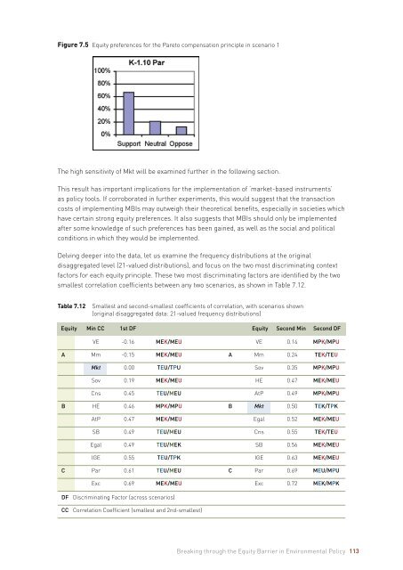
Figure 7.5 <strong>Equity</strong> preferences for <strong>the</strong> Pareto compensation pr<strong>in</strong>ciple <strong>in</strong> scenario 1<br />
The high sensitivity of Mkt will be exam<strong>in</strong>ed fur<strong>the</strong>r <strong>in</strong> <strong>the</strong> follow<strong>in</strong>g section.<br />
This result has important implications for <strong>the</strong> implementation of ‘market-based <strong>in</strong>struments’<br />
as policy tools. If corroborated <strong>in</strong> fur<strong>the</strong>r experiments, this would suggest that <strong>the</strong> transaction<br />
costs of implement<strong>in</strong>g MBIs may outweigh <strong>the</strong>ir <strong>the</strong>oretical benefits, especially <strong>in</strong> societies which<br />
have certa<strong>in</strong> strong equity preferences. It also suggests that MBIs should only be implemented<br />
after some knowledge of such preferences has been ga<strong>in</strong>ed, as well as <strong>the</strong> social and political<br />
conditions <strong>in</strong> which <strong>the</strong>y would be implemented.<br />
Delv<strong>in</strong>g deeper <strong>in</strong>to <strong>the</strong> data, let us exam<strong>in</strong>e <strong>the</strong> frequency distributions at <strong>the</strong> orig<strong>in</strong>al<br />
disaggregated level (21-valued distributions), and focus on <strong>the</strong> two most discrim<strong>in</strong>at<strong>in</strong>g context<br />
factors for each equity pr<strong>in</strong>ciple. These two most discrim<strong>in</strong>at<strong>in</strong>g factors are identified by <strong>the</strong> two<br />
smallest correlation coefficients between any two scenarios, as shown <strong>in</strong> Table 7.12.<br />
Table 7.12<br />
Smallest and second-smallest coefficients of correlation, with scenarios shown<br />
(orig<strong>in</strong>al disaggregated data: 21-valued frequency distributions)<br />
<strong>Equity</strong> M<strong>in</strong> CC 1st DF <strong>Equity</strong> Second M<strong>in</strong> Second DF<br />
VE -0.16 MEK/MEU VE 0.14 MPK/MPU<br />
A Mm -0.15 MEK/MEU A Mm 0.24 TEK/TEU<br />
Mkt 0.00 TEU/TPU Sov 0.35 MPK/MPU<br />
Sov 0.19 MEK/MEU HE 0.47 MEK/MEU<br />
Cns 0.45 TEU/MEU AtP 0.49 MPK/MPU<br />
B HE 0.46 MPK/MPU B Mkt 0.50 TEK/TPK<br />
AtP 0.47 MEK/MEU Egal 0.52 MEK/MEU<br />
SB 0.49 TEU/MEU Cns 0.55 TEK/TEU<br />
Egal 0.49 TEU/MEK SB 0.56 MEK/MEU<br />
IGE 0.55 TEU/TPK IGE 0.63 MEK/MEU<br />
C Par 0.61 TEU/MEU C Par 0.69 MEU/MPU<br />
Exc 0.69 MEK/MEU Exc 0.72 MEK/MPK<br />
DF Discrim<strong>in</strong>at<strong>in</strong>g Factor (across scenarios)<br />
CC Correlation Coefficient (smallest and 2nd-smallest)<br />
<strong>Break<strong>in</strong>g</strong> <strong>through</strong> <strong>the</strong> <strong>Equity</strong> <strong>Barrier</strong> <strong>in</strong> <strong>Environmental</strong> Policy 113