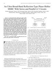
Power Spectrum of Gravitational Waves from Unbound ... - APC

9 th LISA Symposium, Paris 

ASP Conference Series, Vol. 467 

G. Auger, P. Binétruy and E. Plagnol, eds. 

c○ 2012 Astronomical Society of the Pacific 

Power Spectrum of Gravitational Waves from Unbound Compact 

Binaries 

Lorenzo De Vittori, 1 Philippe Jetzer 1 and Antoine Klein 2 

1 University of Zurich, Institute for Theoretical Physics, Switzerland 

2 Montana State University, Departement of Physics, Bozeman, USA 

Abstract. Unbound interacting compact binaries emit gravitational radiation in a 

wide frequency range. Since short burst-like signals are expected in future detectors, 

such as LISA or advanced LIGO, it is interesting to study their energy spectrum and the 

position of the frequency peak. Here we derive them for a system of massive objects 

interacting on hyperbolic orbits within the quadrupole approximation, following the 

work of Capozziello et al. In particular, we focus on the derivation of an analytic 

formula for the energy spectrum of the emitted waves. Within numerical approximation 

our formula is in agreement with the two known limiting cases: for the eccentricity 

ε=1, the parabolic case, whose spectrum was computed by Berry and Gair, and the 

largeε limit with the formula given by Turner. 

1. Theoretical framework 

Since in the last years the Gravitational Waves (GWs) detection technology has improved very 

rapidly, and it is believed that the precision we reached should enable their detection, it is interesting 

to study the dynamics of typical systems and their emission of GWs and in particular 

their frequency spectrum, in order to know at which wave-length range we should expect gravitational 

radiation. 

For the cases of binary systems or spinning black holes on circular and elliptical orbits 

the resulting energy spectra have already been well studied, e.g. Peters & Mathews (1963); 

Peters (1964). The energy spectrum for parabolic encounters has been computed either by 

direct integration along unbound orbits by Turner (1977) or more recently by taking the limit 

of the Peters and Mathews energy spectrum for eccentric Keplerian binaries, see Berry & Gair 

(2010). 

The emission of GWs from a system of massive objects interacting on hyperbolic trajectories 

using the quadrupole approximation has been studied by Capozziello et al. (2008) and 

analytic expressions for the total energy output derived. However, the energy spectrum has 

been computed only for the large eccentricity (ε≫1) limit, see in Turner (1977). Here we 

present the work done in the last year, De Vittori et al. (2012). We derive the energy spectrum 

for hyperbolic encounters for all valuesε≥1 and we give an analytic expression for it in terms 

of Hankel functions. 

GWs are solutions of the linearized field equations of General Relativity and the radiated 

power to leading order is given by Einstein’s quadrupole formula, as follows 

P= G 

45 c 5〈 ¯D i j 

¯D i j 〉, (1) 

where we used as definition for the second moment tensors M i j := 1 c 2 ∫ 

T 00 x i x j d 3 x, and for the 

quadrupole moment tensor D i j := 3M i j −δ i j M kk and where ¯D stands for the third derivative 

of D. The quantity M i j depends on the trajectories of the involved masses, and can easily 

331

332 De Vittori, Jetzer and Klein 

be computed for all type of Keplerian trajectories. To compute the power spectrum, i.e. the 

amplitude of radiated power per unit frequency, requires a Fourier transform of equation (1), 

which is rather involved (for the elliptical case see e.g. Maggiore (2008)), and we will derive it 

below for hyperbolic encounters. The eccentricityεof the hyperbola is 

√ 

ε := 1+2E L 2 /µα 2 , (2) 

where E = 1 2 µ v2 0 

(E is a conserved quantity for which we can take the energy at t=−∞), 

v 0 being the velocity of the incoming mass m 1 at infinity, the angular momentum L=µ b v 0 , 

the impact parameter b, the reduced massµ := m 1 m 2 

m 1 +m 2 

, the total mass m := m 1 + m 2 , and the 

parameterα := G mµ. 

Setting the angle of the incident body toϕ=0 at initial time t=−∞, the radius of the 

trajectory as a function of the angle and as a function of time is given by 

a (ε 2 − 1) 

r(ϕ)= , r(ξ)=a (ε coshξ−1) (3) 

1+ε cos(ϕ−ϕ 0 ) 

√ 

µ a 

with the time parametrized byξ through the relation t(ξ)= 

3 

α 

(ε sinhξ−ξ), whereξ goes 

from−∞ to+∞. Expressing this in Cartesian coordinates in the orbital plane, we finally get the 

equations for hyperbolic trajectories 

x(ξ)=a (ε− coshξ), y(ξ)=a √ ε 2 − 1 sinhξ. (4) 

2. Power spectrum of Gravitational waves from hyperbolic paths 

2.1. Power emitted per unit angle 

In Capozziello et al. (2008) the computation of the power emitted as a function of the angle, as 

well as the total energy emitted by the system has been already carried out. They turn out to be: 

P(ϕ)=− 32 G L6 µ 2 

45 c 5 b 8 f (ϕ,ϕ 0 ), ∆E= 32 Gµ2 v 5 0 

b c 5 F(ϕ 0 ), (5) 

where for the factors f (ϕ,ϕ 0 ) and F(ϕ 0 ) one finds: 

f (ϕ,ϕ 0 )= sin(ϕ 0− ϕ 2 )4 sin( ϕ 2 )4 ( 

· 150+72 cos(2ϕ 

tan(ϕ 0 ) 2 sin(ϕ 0 ) 6 0 )+ 66 cos(2(ϕ 0 −ϕ)) 

) 

−144 (cos(2ϕ 0 −ϕ)−cos(ϕ)) , 

F(ϕ 0 )= 

1 

720 tan 2 ϕ 0 sin 4 ϕ 0 

× [2628ϕ 0 + 2328ϕ 0 cos 2ϕ 0 

+144ϕ 0 cos 4ϕ 0 − 1948 sin 2ϕ 0 − 301 sin 4ϕ 0 ]. 

This means that the total radiated energy of the system can be determined knowing the parameters 

b and v 0 , and of course the reduced massµ. 

2.2. Power spectrum 

We compute now P(ω), the Fourier transform of P(t), which describes the distribution of the 

amplitude of the power emitted in form of GWs depending on the frequency. In Landau & 

Lifshitz (1967) and Longair (2011) some hints are given when solving the analogous problem 

in electrodynamics. The crucial idea is to use Parseval’s theorem on the integration of Fourier 

(6) 

(7)

Power Spectrum of Gravitational Waves from Unbound Compact Binaries 333 

transforms, and then to express some quantities in terms of Hankel functions. This allows to get 

in an easier way the function P(ω), for which we use the expression given in eq. (1) 

∫ 

∆E= 

∫ 

P(t)dt= 

P(ω)dω=− G ∫ 

〈 ¯D 

45c 5 i j (t) ¯D i j (t)〉 dt 

=− G ∫ 

(|̂¯D 

45c 5 11 (ω)| 2 +|̂¯D 22 (ω)| 2 + 2|̂¯D 12 (ω)| 2 +|̂¯D 33 (ω)| 2 ) dω, 

(8) 

wherê¯D i j (ω) is the Fourier transform of ¯D i j (t). It is easy to see that the last equation 

represents the total amount of energy dissipated in the encounter. Therefore, the integrand in 

the last line has to be equal to the power dissipated per unit frequency P(ω) : 

P(ω)=− G 

45c 5 ( |̂¯D 11 (ω)| 2 +|̂¯D 22 (ω)| 2 + 2|̂¯D 12 (ω)| 2 +|̂¯D 33 (ω)| 2) . (9) 

As next, we need to compute thê¯D i j (ω), take the square their norm and add them together, 

which yields the power spectrum. Computing the D i j explicitly - keeping in mind that we use 

the time parametrization t(ξ)= √ µ a 3 /α (ε sinhξ−ξ) - we get: 

D 11 (t)∼((3−ε 2 ) cosh 2ξ− 8εcoshξ), (10) 

D 22 (t)∼(4εcoshξ+ (2ε 2 − 3) cosh 2ξ), (11) 

D 33 (t)∼(4εcoshξ+ε 2 cosh 2ξ), (12) 

D 12 (t)∼(2εsinhξ− sinh 2ξ). (13) 

The Fourier transform of the third derivatives of D i j (t) is given bŷ¯D i j (ω)=iω 3̂D i j (ω), 

thus we have just to computêD i j (ω). We can closely follow the calculations performed in 

Landau & Lifshitz (1967), where the similar problem in electrodynamics of the emitted power 

spectrum for scattering charged particles on hyperbolic orbits is treated. In particular the following 

Fourier transforms are used (for their derivation see Appendix A in De Vittori et al. 

(2012)). 

sinhξ=− ̂ 

π ωε H(1) iν (iνε), ĉoshξ=−π ω H(1)′ iν 

(iνε), (14) 

H (1)′ 

˜α (x)= 1 2 (H(1) ˜α−1 

(x)− H(1) 

˜α+1 

(x)), (15) 

where H (1) 

˜α 

(x) is the Hankel function of the first kind of order ˜α, and whereνis defined as 

ν :=ω √ µa 3 /α. 

Taking the D i j (t) from above we get 

̂D 11 (ω)= a2 mπ 

[16ε H(1)′ 

4ω 

iν (iνε)+(ε2 − 3) H (1)′ 

iν 

(iνε/2)], (16) 

̂D 22 (ω)= a2 mπ 

4ω [(3−2ε2 ) H (1)′ 

iν 

(iνε/2)−8ε H(1)′ 

iν 

(iνε)], (17) 

̂D 33 (ω)= a2 mπ 

[8ε H(1)′ 

iν (iνε)+ε2 H (1)′ 

iν 

(iνε/2)], (18) 

̂D 12 (ω)= 3 a2 mπ 

4ωε 

4ω 

√ 

ε2 − 1 [H (1) 

iν 

(iνε/2)−4ε H(1) 

iν 

(iνε)]. (19) 

Inserting this result into eq. (9), and using the formula for the Fourier transform of the third 

derivative, we get the power spectrum of the gravitational wave emission for hyperbolic encounters


where the function F ε (ω) turns out to be 

P(ω)=− G a4 m 2 π 2 

720 c 5 ω 4 F ε (ω), (20) 

F ε (ω)=|[16ε H (1)′ 

iν (iνε)+(ε2 − 3) H (1)′ 

iν (iνε/2)]| 2 + 

|[(3−2ε 2 ) H (1)′ 

iν 

(iνε/2)−8ε H(1)′ 

iν (iνε)]| 2 +|[8ε H (1)′ 

iν (iνε)+ 

ε 2 H (1)′ 

iν (iνε/2)]| 2 + 9 (ε2 − 1) 

ε 2 |[H (1) 

iν 

(iνε/2)− 4ε H(1) 

iν (iνε)]| 2 . 

(21) 

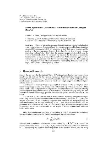
In Fig. 1 the functionω 4 F ε (ω) is plotted for some some values ofε: this is the frequency 

power spectrum of gravitational radiation emitted by an hyperbolic encounter. Unfortunately the 

expression for F ε (ω) is rather complicated and we could not find an analytical way to simplify 

it. We thus made some numerical tests to check its validity and clearly the integral of (20) has 

to be equal to∆E in (5), which was obtained by integrating over the power emitted per unit 

frequency, i.e. ∫ ∞ 

P(ω) dω=∆E. 

0 

We have checked the validity of this equality for different sets of values, comparable to 

those used in Capozziello et al. (2008), e.g. b=1AU, v 0 = 200 km/s, and m 1,2 = 1.4 M ⊙ , or 

similar. For all of these sets we got agreement within numerical accuracy. 

More interesting is the case where the eccentricity approachesε=1. According to eq. (2) 

this is the case e.g. with the set of initial conditions b=2 AU, v 0 = 6.4 km/s and m 1,2 = 1.4 M ⊙ . 

Since this is a limit case for a parabolic trajectory, we can directly compare our result with the 

one studied by Berry & Gair (2010), and indeed they coincide, within numerical accuracy. For a 

discussion about the feasibility of an analytical comparison see Appendix B in De Vittori et al. 

(2012). 

Finally, we turn to the largeεlimit and compare our result with the one given in Turner 

(1977) and Wagoner & Will (1976). The expression for the total energy emitted during an 

hyperbolic interaction is written in Turner (1977) as: 

∆E T = 8 G 7/2 m 1/2 m 2 1 m2 2 

15 c 5 r 7/2 

min 

g(ε), where forε→∞: 

g(ε)∼ 37π 

8 

√ ε +O(ε −1/2 ), (22) 

which also agrees with the result of Wagoner & Will (1976). 

Comparing our total energy from the quadrupole approximation, eq. (5), with the expression 

for the energy∆E T (22) by Turner (1977) valid in the largeεlimit, we see that they 

coincide for large eccentricities, having e.g. a 1% difference afterε=100, and a 5% difference 

afterε=20. For a more detailed discussion about these comparisons with previous results, see 

our full work De Vittori et al. (2012). 

3. Conclusions 

Short gravitational wave burst-like signals are expected in the data stream of detectors. Although 

these signals will likely be too short to allow us to measure the parameters of the emitting 

system accurately, the results presented in this paper could be used to get a rough estimate 

of these parameters, by observing the position of the peak, the amount of energy released and 

the timescale of the interaction. 

Given the knowledge of the power spectrum we can easily see which kind of hyperbolic 

encounters could generate gravitational waves detectable e.g. with eLISA, advanced LIGO 

or advanced VIRGO. Measurements from unbound interactions with ground-based detectors 

could in principle be possible, though the energy emitted at e.g. ±200 Hz is below the minimum 

threshold for advanced LIGO or advanced VIRGO, making detections unlikely but not 

impossible. The space-based interferometer instead is expected to cover frequencies ranging

Power Spectrum of Gravitational Waves from Unbound Compact Binaries 335 

1.0 

0.8 

PΩ 

0.6 

0.4 

0.2 

0.0 

0 0.1 0.2 0.3 0.4 0.5 0.6 0.7 

Ω 

Figure 1. The frequency power spectrum of gravitational radiation emitted by an 

hyperbolic encounter. On the x-axis we have the angular frequencyωexpressed 

in mHz units, whereas on the y-axis the amplitude of P(ω) is normalized to the 

maximum value of theε∼2.5 case. These are the expected emissions generated 

by a system of two supermassive black holes with m=10 7 M ⊙ , impact parameter 

b=10 AU, and different relative velocities. With lower velocities the interactions 

are stronger and the eccentricity decreases. These spectra, in order from the highest 

to the lowest, represent systems with v 0 = 3.4×10 7 m/s (ε∼2.5), v 0 = 3.5×10 7 m/s 

(ε∼3), v 0 = 3.6×10 7 m/s (ε∼3.1), v 0 = 3.75×10 7 m/s (ε∼3.4), v 0 = 4×10 7 m/s 

(ε∼3.8), v 0 = 4.5×10 7 m/s (ε∼4.7), respectively. In particular the case withε∼3 

(plotted with the dashed line) is discussed in the conclusions. As one can see, for 

higher eccentricities the peak frequency slowly decreases. This is only true for values 

of v 0 up to∼ 6×10 7 m/s, whereas above it increases again. Moreover, decreasing the 

mass or increasing the impact parameter changes the eccentricity as well. We should 

be able to detect incoming waves in that range e.g. with eLISA, since the peak at 

∼ 0.2 mHz fits in its observable band. For a more detailed discussion see Sec. 3 and 

e.g. Bender et al. (2003). 

from 0.03 mHz up to 1 Hz, see e.g. Bender et al. (2003), where the interactions could release 

more energy. 

An unbounded collision between two intermediate-mass black holes, let’s say of 10 3 M ⊙ 

each, with an encounter velocity of 2000 km/s at a distance of 1 AU, would generate, according 

to our eq. (20), a frequency spectrum with peak around 0.04 mHz, with 80% of the emission in 

the range between 0.01 and 0.07 mHz, i.e. in the lower range limit of eLISA. Another possible 

example of measurable impact would be an encounter between two supermassive black holes 

with mass, e.g., comparable to the expected mass of Sagittarius A*, the black hole believed 

to be at the center of our galaxy, i.e. ∼ 10 7 M ⊙ . With a distance of some AU, and a high 

velocity (we want to exclude the bounded case) of tens of thousands km/s, such a collision 

would generate an energy spectrum with peak at∼ 0.2 mHz with 80% between 0.03 and 0.37 

mHz, thus in the observable range of eLISA. (Its energy spectrum is plotted with a dashed line 

in Fig. 1.) Estimates for the rate of such events have been considered e.g. in Capozziello & De 

Laurentis (2008). They consider e.g. typical compact stellar cluster around the Galactic Center,


and expect an event rate of 10 −3 up to unity per year, depending on the radius of the object and 

the amount of such clusters in the near region. 

We believe that with the energy spectrum found here one should be able to classify the 

different encounters depending on t different encounters depending on the detected shape, and 

therefore get a better insight into the map of our galaxy or the near universe. 

Acknowledgments. We thank N. Straumann for useful discussions and for bringing to our 

attention the relevant treatment of the hyperbolic problem in electrodynamics in Landau & 

Lifschitz. We also thank L. Blanchet for his encouragement and for pointing out the possibility 

of treating the same problem in another way. Finally, we would also like to thank C. Berry for 

helping clarifying some details. 

References 

Bender, P., et al. 2003, LISA laser interferometer space antenna: a cornerstone mission for the 

observation of gravitational waves, Tech. rep., ESA-SCI 

Berry, C., & Gair, J. 2010, Phys. Rev. D, 82, 10751 

Capozziello, S., & De Laurentis, M. 2008, Astroparticle Physics, 30, 105 

Capozziello, S., De Laurentis, M., De Paolis, F., Ingrosso, G., & Nucita, A. 2008, 

Mod.Phys.Lett.A 23:99-107 

De Vittori, L., Jetzer, P., & Klein, A. 2012, Phys. Rev. D, 86, 044017 

Landau, L., & Lifshitz, E. 1967, Theoretical Physics: Classical Theory of Fields 

Longair, M. 2011, High Energy Astrophysics 

Maggiore, M. 2008, Gravitational Waves. Vol. I: Theory and Experiments (Oxford University 

Press) 

Peters, P. 1964, Phys. Rev., 136, B1224 

Peters, P., & Mathews, J. 1963, Phys. Rev., 131, 435 

Turner, M. 1977, Astrophysical Journal, 216, 610-619 

Wagoner, R., & Will, C. 1976, Astrophysical Journal, 210, 764

Power Spectrum of Gravitational Waves from Unbound ... - APC

You also want an ePaper? Increase the reach of your titles

Delete template?

Save as template?