Evaluation of a Rigidity Penalty Term for Nonrigid Registration - elastix

Evaluation of a Rigidity Penalty Term for
Nonrigid Registration
Marius Staring, Stefan Klein and Josien P.W. Pluim
Image Sciences Institute, University Medical Center Utrecht,
P.O. Box 85500, 3508 GA, Room Q0S.459, Utrecht, The Netherlands,
{marius,stefan,josien}@isi.uu.nl
Abstract
Nonrigid registration of medical images usually does not model properties of
different tissue types. This results for example in nonrigid deformations of
structures that are rigid. In this work we address this problem by employing
a local rigidity penalty term. We illustrate this approach on a 2D synthetic
image, and evaluate it on clinical 2D DSA image sequences, and on
3D CT follow-up data of the thorax of patients suffering from lung tumours.
The results show that the rigidity penalty term does indeed penalise nonrigid
deformations of rigid structures, whereas the standard nonrigid registration
algorithm compresses those.
1 Introduction
Nonrigid registration of patient data is an important technique in the field of medical
imaging. One of the remaining problems of nonrigid registration algorithms is that usually
everything in the images is treated as nonrigid tissue, even objects that are clearly rigid,
or objects for which it is desired to keep them rigid. Examples of the first are bones
and surgical instruments. Examples of the second include structures that contain contrast
material, visible in one image, but not in the other. Standard intensity based nonrigid
registration algorithms will typically give undesired compression of these structures [10,
15]. It is necessary to prevent nonrigid behaviour of these local structures, and keep them
rigid instead.
In the literature several methods have been described to constrain deformations. The
employment of a regularisation or penalty term is a well-known strategy. Examples of
such terms are the bending energy of a thin plate [12], the linear elasticity constraint
[1, 2] and the incompressibility constraint [10]. Particular methods to enforce rigidity
on structures have also been proposed. Tanner et al. [15] propose to couple the control
points of a B-spline deformation. Another approach is taken by Little et al. [6], who use
modified basis functions describing the deformation, constraining the nonlinear part of
the deformation at rigid locations by multiplication with a weight function.
Recently, some approaches similar to our own were published [7, 11], in which rigidity
is enforced by penalising deviation of the Jacobian from being orthonormal. In this
paper we propose a penalty term that is capable of penalising locally nonrigid transformations,
which we call a rigidity penalty term. It is based on three criteria a transformation

must meet in order to be locally rigid: linearity of the transformation, and orthonormality
and properness of the Jacobian of the transformation. First results of the method were
published previously [14].
In the following section we describe the rigidity penalty term. Standard nonrigid
registration is compared against registration using the rigidity penalty term in Section 3.
We end with a discussion in Section 4.
2 Method
Registration of a moving image M(x) : Ω M ⊂ R d ↦→ R to a fixed image F(x) : Ω F ⊂ R d ↦→
R, both of dimension d, consists of finding a deformation u(x) that makes M(x + u(x))
spatially aligned to F(x). The quality of alignment is defined by a similarity or distance
measure D, such as the sum of squared differences (SSD), the correlation ratio, or the
mutual information (MI) measure.
Because this problem is ill-posed, a regularisation term or smoother S is introduced
and the registration problem is formulated as an optimisation problem in which a cost
function J is minimised w.r.t. u, with:
J [F,M; u]=D[F,M; u]+αS [u], (1)
where α weighs similarity against smoothness. Note that at the minimum the derivatives
of the similarity measure and the regularisation term are not necessarily zero. Merely, a
balance is found between the two, which is influenced by the parameter α. Therefore, the
penalty term can not be considered a hard constraint, but it is sometimes referred to as a
soft constraint.
In [14] we propose a penalty term S rigid [u] that penalises nonrigid deformations of
rigid objects, which we call the rigidity penalty term. This penalty term can be weighted
locally, so that some parts of the image are restricted to rigid movement, while other parts
are penalised partially or are allowed to deform freely.
2.1 Registration Algorithm
We employ a registration framework largely based on the papers of Rueckert et al. [12]
and Mattes et al. [8]. The similarity measure is the mutual information measure using
an implementation by Thévenaz and Unser [16]. The deformation field is parameterised
by cubic B-splines. A multiresolution approach is taken to avoid local minima, using a
Gaussian pyramid with a subsampling factor of two in each dimension. We also employ
a multiresolution approach of the deformation grid: when the image resolution in the
pyramid is doubled, the B-spline control point spacing is halved. For the optimisation
of the cost function J , we employ a stochastic gradient descent optimiser, using only a
small, randomly chosen portion of the total number of pixels for calculating the derivative
of J with respect to the B-spline parameters [5].
2.2 Construction of the Rigidity Penalty Term
The rigidity penalty term S rigid [u] is constructed by penalising deviation from three conditions.
For a deformation field u to be rigid, it must hold that u(x)+x = Rx + t, with R

and t a rotation matrix and a translation vector, respectively. Note that the rotation matrix
R is the Jacobian of the transformation u(x)+x. The three conditions are (given in 2D
for readability):
linearity of u(x), stating that the second order derivatives are zero:
LC ki j (x)= ∂ 2 u k (x)
= 0, (2)
∂x i ∂x j
for all k,i, j = 1,2, not counting duplicates.
orthonormality of R, which can be expressed in terms of derivatives of u(x):
2
( )( )
∂uk (x) ∂uk (x)
OC ij (x)= ∑ + δ ki + δ kj − δ ij = 0, (3)
k=1
∂x i
∂x j
for all i, j = 1,2, again not counting duplicates.
properness of R: PC(x) =det(R) − 1 = 0, which can again be expressed in terms of
derivatives of u(x). Note that this condition basically amounts to an incompressibility
constraint, see also [10].
We define the rigidity penalty term S rigid [u] to be the sum of these conditions squared.
In order to distinguish between rigid and nonrigid tissue, the penalty term is weighted by
a so-called rigidity coefficient c(x) ∈ [0,1] of the tissue type at position x. The complete
expression reads:
{
S rigid [
[u] ∑ c(x) ∑ LCki j (x) ] 2 + ∑[OC ij (x)] 2 +[PC(x)]
}. 2 (4)
x∈Ω F k,i, j
i, j
The rigidity coefficient c(x) is equal to zero for pixels x in completely nonrigid tissue,
thereby not penalising deformations at those locations. For completely rigid tissue c(x)
is set to one. For other tissue types a value of c(x) is chosen between zero and one.
The rigidity coefficient image can be constructed by performing a manual or automatic
segmentation of structures of interest, after which rigidity coefficients can be assigned.
Depending on the application, different methods to create the rigidity coefficient image
can be considered. For the case of CT images the Hounsfield unit might be used, rescaled
to the range [0,1], since more rigid tissue usually has a higher attenuation value.
In [14] we argue the validity of this rigidity penalty term by showing that S rigid [u]=0
if and only if the deformation field u(x) is locally rigid. The linearity term might be
dropped, since it can be shown that orthonormality implies linearity. However, it might
aid the penalty term by guiding the optimisation path. The proposed constraint is not
dependent on the B-spline parameterisation of the deformation field. However, from a
computational point of view, we can benefit from this parameterisation by evaluating the
rigidity penalty term only over the control points. For details we refer to [14].
3 Experiments and Results
Standard nonrigid registration using only the similarity term, as described in Section 2.1,
is compared with nonrigid registration using the rigidity penalty term. The two methods

(a) (b) (c)
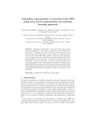
Figure 1: Comparison of registration with and without S rigid [u] for a 2D synthetic example.
The white square is to be kept rigid. (a) fixed image (lower) and moving image
(upper), (b) resulting deformation field of standard registration, and (c) resulting deformation
field including the rigidity constraint.
are illustrated on synthetic images. They are compared on clinical data, viz. 3D CT
follow-up data of the thorax containing lung tumours, and on 2D DSA image data of
different parts of the body. The computation time for registration with the rigidity penalty
term increases about 50% in 2D and about 80% in 3D with a B-spline grid spacing of
eight voxels.
All experiments were performed with software (www.isi.uu.nl/Elastix/) developed
by the authors. This registration package is largely based on the Insight Segmentation
and Registration Toolkit [4].
3.1 2D Synthetic Example
Rotation of a rigid object is illustrated with the square in Figure 1, where the background
represents nonrigid tissue and the square a rigid object. The rigidity coefficient c(x) is set
to 1.0 on the square and 0.0 elsewhere.
Both algorithms give near perfect registration results for the matching of the squares
in Figure 1. However, the underlying deformation field is highly nonlinear if no rigidity
penalty term is used. By including the penalty term the deformation field is almost perfectly
rigid at the rigid part. This is also reflected in the rigidity constraint S rigid [u], which
has a value of 2.21×10 2 for standard nonrigid registration and a value of 1.28×10 −3 for
registration using the rigidity constraint. The rigidity constraint is not perfectly zero, because
some B-spline control points outside the square, but influencing the points within
the square, are not set to be rigid.
3.2 3D CT Follow-up
In order to compare 3D CT follow-up data by visual inspection of the difference image,
the data sets must be registered nonrigidly. We have five CT follow-up data sets of
the thorax available, of patients suffering from lung tumours, collected at the Radiology
department of the University Medical Centre Utrecht. The images are acquired under

(a) (b) (c)
(d) (e) (f)
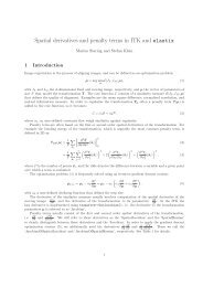
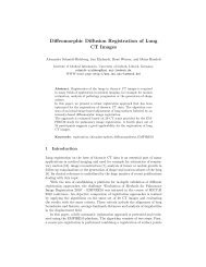
Figure 2: Comparison of both nonrigid registration methods for a slice taken from 3D
CT thorax images. The tumours, located within the box (see (d)), have to be kept rigid
for diagnostic reasons. (a) and (d): CT slice at time t 0 (the fixed image) and time t 1
(the moving image), respectively, (b) and (c): difference of the result of similarity only
nonrigid registration with the fixed image, and a part of the resulting deformation field,
respectively, (e) and (f): the same for nonrigid registration using S rigid [u].
breath-hold with a Philips 16 slice spiral CT scanner (Mx8000 IDT 16). The data are
of size 512 × 512 by 400 - 550 slices, have voxel sizes of around 0.7 × 0.7 × 0.7 mm,
and are resized by a factor of 2 in each dimension before registration. The five data sets
contain 36 tumours in total, with an average volume of 2.5 ml for the first scan and 5.1 ml
at the second. The CT image taken at time t 0 is set to be the fixed image, the follow-up
CT image (time t 1 ) the moving image. For visual inspection of the tumour growth from
the difference image, the tumours must not deform nonrigidly, but only in a rigid fashion.
This way tumour growth can be seen from the difference image, in relation with the
anatomy shown in the CT image. For an example of the difference image in these cases,
see Figure 2(b) and 2(e). Tumour growth is effectively concealed in the similarity only
based registration.
To get a coarse alignment between fixed and moving image a rigid registration is performed
first. Then the nonrigid registration is performed, using a B-spline grid spacing of
8 voxels, 4 resolutions, 300 iterations per resolution, and 5000 voxel samples to calculate
(the derivative of) the mutual information. For the nonrigid registration with the rigidity
penalty term, the tumour regions are defined by a crude manual delineation, setting

Table 1: Average lung overlap.
before registration rigid similarity only with S rigid [u]
0.64 ± 0.22 0.91 ± 0.06 0.98 ± 0.01 0.97 ± 0.02
c(x)=1.0 in the tumour regions and 0.0 elsewhere.
Accuracy of the registration is measured by calculating the lung overlap of the registered
image with the fixed one. For this purpose automatic lung segmentations are made
with an algorithm based on the method by Hu et al. [3,13]. The overlap measure is defined
as
overlap 2 ·|L 1 ∩ L 2 |
|L 1 | + |L 2 | , (5)
where L i is the set of all voxels from the lung, and where |L i | is the size of set L i . From
the results reported in Table 1, we see that both registrations lead to good lung overlap.
Employing a rigidity penalty term, constrains the deformation, leading to a slightly less
accurate lung overlap. Because of the (compact) support of the B-splines, a boundary
around the tumour is influenced by the control points within the tumour. The extent of
this boundary can be controlled with the B-spline grid spacing.
Manual segmentations of the tumours are used to evaluate their rigidity. Tumour volume
measurements are performed to see if the registration is at least volume preserving.
In order to compare tumours volumes with different sizes we can not use the arithmetic
mean, because large tumours influence the arithmetic mean disproportionally. Therefore,
volume growth ratios are calculated, where every tumour volume is divided by its volume
at t 1 . For growth ratios it is better to use the geometric mean and the geometric standard
deviation, which are defined as:
√
n
µ g = n ∏r i ,
i=1
σ g = exp
(√
1
n
n
∑
i=1
(lnr i − ln µ g ) 2 ), (6)
where r i denotes the growth ratio of tumour i. We report the geometric mean growth
ratios and standard deviations in Table 2. It can be appreciated that volume is much better
preserved when applying the rigidity penalty term, compared to similarity only based
registration. Part of the residual volume difference can be explained by interpolation
artifacts due to resampling, as can be seen from the results for rigid registration. From
the deformation field, see Figure 2(f) (compare with 2(c)) is can also be appreciated that
nonrigid registration using the rigidity penalty term preserves rigidity locally.
3.3 Digital Subtraction Angiography
Evaluation is also performed on 2D clinical digital X-ray angiography image data, acquired
with an Integris V3000 C-arm imaging system (Philips). Digital Subtraction Angiography
(DSA) imaging often suffers from motion artifacts, due to motion of or within
the patient, see Figure 3(a) - 3(c). Nonrigid registration is needed to compensate for this.
We have 26 image sequences available of twelve different patients, each containing about
10 images. Images are mostly of size 512×512 and are taken of different locations in the

Table 2: Geometric mean tumour volume ratios. Geometric means are calculated for four
growth groups and for all growth ratios. The second group for example is the group of
tumours that corresponds to a volume ratio t 1 /t 0 between 1 and 3/2.
group t 1 /t 0 t 0 rigid similarity only with S rigid [u]
(0,1] 1.18 ×/ 1.08 0.99 ×/ 1.02 1.00 ×/ 1.03 0.96 ×/ 1.06
( ]
1,
3
2
0.84 ×/ 1.05 0.96 ×/ 1.04 0.97 ×/ 1.05 1.03 ×/ 1.03
( 32
,3 ] 0.48 ×/ 1.10 1.00 ×/ 1.02 0.79 ×/ 1.07 1.00 ×/ 1.02
(3,∞) 0.23 ×/ 1.13 1.02 ×/ 1.03 0.69 ×/ 1.12 0.99 ×/ 1.02
all 0.52 ×/ 1.29 0.99 ×/ 1.03 0.83 ×/ 1.10 1.00 ×/ 1.03
body, such as the abdomen, the brain, neck and lungs. Because it takes time for the contrast
bolus to travel through the vasculature, different parts of the vasculature are visible
at different times. If the whole vasculature is to be extracted, all images have to be registered
to some baseline image. For this, we choose the first image in each sequence, which
is taken before arrival of the contrast bolus, to be the fixed image. For this experiment
we register only one of the other images to the fixed image: the image showing most of
the vasculature is chosen as the moving image. The nonrigid registration of DSA images
can lead to undesired compression of the vasculature, as reported in [9] for CT-DSA. Although
the vessels are not intrinsically rigid, they are to be kept rigid, since there exists
no information to do otherwise: vessels are visible in one image and not in the other.
We applied a rigid registration first for coarse alignment. For the nonrigid registration
we use a B-spline grid spacing of 16 pixels, 2 resolutions, 600 and 300 iterations per
resolution, and 5000 samples for calculating (the derivative of) the MI. A crude manual
segmentation of the vessels is used for defining c(x).
To measure the success of the nonrigid registration, the Mean Square Difference
(MSD) of the background B is calculated. The MSD is defined as:
MSD = 1 (
|B| ∑
2
F(x) − M(x + u(x)))
. (7)
x∈B
Results are shown in the top row of Table 3, showing improvement of this measure for
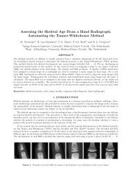
nonrigid registration. Compare also Figure 3(d) with Figure 3(e) and 3(e). As a measure
of rigidity, vessel diameter measurements are carried out to quantify vessel compression.
In every one of the 26 images six diameter measurements are carried out. The geometric
mean of the vessel diameter ratios are reported in the bottom row of Table 3. Without
employing the rigidity penalty term the vessels are severely compressed, which is avoided
with the use of S rigid [u]. The shape of the deformation fields confirms this, see Figure
3(g) and 3(g).
4 Conclusions and Discussion
We have proposed a method to perform nonrigid registration, while keeping user-defined
local structures rigid. This is achieved by adding a rigidity penalty term to the registration

(a) (b) (c)
(d) (e) (f)
(g)
(h)
Figure 3: Comparison of different registration algorithms for 2D DSA images. The vessels
are to be kept rigid, while motion artifacts are to be reduced by the registration. (a)
DSA baseline image: the fixed image, (b) DSA image after injection of the contrast bolus:
the moving image, (c) - (f) are difference images with the fixed image, (c) with the moving
image, (d) with the result of rigid registration, (e) with the result of similarity only
nonrigid registration, (f) with the result of nonrigid registration using the rigidity penalty
term. The bottom row depicts parts of the resulting deformation field of similarity only
(g), and using the rigidity penalty term (h). The black box in Figure (e) and (f) denotes
the part of the deformation field that is depicted.
framework (1). The method is illustrated on a synthetic 2D example and evaluated on 2D
and 3D clinical data.

Table 3: Results for DSA. Arithmetic means for the MSD and geometric means for the
vessel diameter ratios compared with t 1 .
no registration rigid similarity only with S rigid [u]
MSD 231 ± 205 215 ± 181 163 ± 105 171 ± 128
diameter 1.00 ×/ 1.00 1.00 ×/ 1.00 0.85 ×/ 1.07 0.99 ×/ 1.01
From the results we can see that the rigidity penalty term indeed penalises nonrigid
deformations, but complete rigidity is sometimes not achieved. Some reasons are the
following. 1) The rigidity penalty term is not a hard constraint, it is merely a tradeoff
between similarity and penalty. 2) For the case of modelling the deformation field with
cubic B-splines, the control points outside a rigid structure influence the inside. Therefore,
if complete rigidity is wanted, the two adjacent control points outside the structure must
also be kept rigid, for example by performing a dilation on the rigidity coefficient image
c(x). Of course the inverse is also true: the rigid part influencing the nonrigid part, thereby
restricting the deformation at the boundaries of the rigid structure. The extent of this
boundary is controlled by the B-spline control point spacing.
The linearity condition (2) might not be necessary, since it can be shown that orthonormality
of the Jacobian of u implies linearity of u. However, it might guide the optimiser
in reaching rigidity; this is interesting future work.
Acknowledgments
This research was funded by the Netherlands Organisation for Scientific Research (NWO).
This work also benefited from the use of the Insight Segmentation and Registration Toolkit
(ITK). We gratefully acknowledge Oskar Škrinjar for a fruitful discussion about the linearity
condition of the rigidity penalty term.
References
[1] G. E. Christensen and H. J. Johnson. Consistent image registration. IEEE Transactions
on Medical Imaging, 20(7):568 – 582, 2001.
[2] B. Fischer and J. Modersitzki. A unified approach to fast image registration and a
new curvature based registration technique. Linear Algebra and its Applications,
380:107 – 124, 2004.
[3] S. Hu, E. A. Hoffman, and J. M. Reinhardt. Automatic lung segmentation for accurate
quantitation of volumetric X-Ray CT images. IEEE Transactions on Medical
Imaging, 20(6):490 – 498, 2001.
[4] Luis Ibáñez, Will Schroeder, Lydia Ng, and Josh Cates. The ITK Software Guide.
Kitware, Inc. ISBN 1-930934-15-7, second edition, 2005.
[5] S. Klein, M. Staring, and J. P. W. Pluim. Comparison of gradient approximation
techniques for optimisation of mutual information in nonrigid registration. In SPIE

Medical Imaging: Image Processing, volume 5747, pages 192 – 203. SPIE Press,
2005.
[6] J. A. Little, D. L. G. Hill, and D. J. Hawkes. Deformations incorporating rigid
structures. Computer Vision and Image Understanding, 66(2):223 – 232, 1997.
[7] D. Loeckx, F. Maes, D. Vandermeulen, and P. Suetens. Nonrigid image registration
using free-form deformations with a local rigidity constraint. In MICCAI, volume
3216 of Lecture Notes in Computer Science, pages 639 – 646. Springer Verlag, 2004.
[8] D. Mattes, D. R. Haynor, H. Vesselle, T. K. Lewellen, and W. Eubank. PET-CT
image registration in the chest using free-form deformations. IEEE Transactions on
Medical Imaging, 22(1):120 – 128, 2003.
[9] T. Rohlfing and C. R. Maurer Jr. Intensity-based nonrigid registration using adaptive
multilevel free-form deformation with an incompressibility constraint. In MICCAI,
volume 2208 of Lecture Notes in Computer Science, pages 111 – 119. Springer
Verlag, 2001.
[10] T. Rohlfing, C. R. Maurer Jr., D. A. Bluemke, and M. A. Jacobs. Volume-preserving
nonrigid registration of MR breast images using free-form deformation with an incompressibility
constraint. IEEE Transactions on Medical Imaging, 22(6):730 –
741, 2003.
[11] D. Ruan, J. A. Fessler, M. Roberson, J. Balter, and M. Kesler. Nonrigid registration
using regularization that accomodates local tissue rigidity. In SPIE Medical
Imaging: Image Processing, volume 6144, pages 346 – 354. SPIE Press, 2006.
[12] D. Rueckert, L. I. Sonoda, C. Hayes, D. L. G. Hill, M. O. Leach, and D. J. Hawkes.
Nonrigid registration using free-form deformations: Application to breast MR images.
IEEE Transactions on Medical Imaging, 18(8):712 – 721, 1999.
[13] I. C. Sluimer, M. Prokop, and B. van Ginneken. Towards automated segmentation
of the pathological lung in CT. IEEE Transactions on Medical Imaging, 24(8):1025
– 1038, 2005.
[14] M. Staring, S. Klein, and Josien P. W. Pluim. Nonrigid registration using a rigidity
constraint. In SPIE Medical Imaging: Image Processing, volume 6144 of Proceedings
of SPIE, pages 355 – 364. SPIE Press, 2006.
[15] C. Tanner, J. A. Schnabel, D. Chung, M. J. Clarkson, D. Rueckert, D. L. G. Hill, and
D. J. Hawkes. Volume and shape preservation of enhancing lesions when applying
nonrigid registration to a time series of contrast enhancing MR breast images. In
MICCAI, volume 1935 of Lecture Notes in Computer Science, pages 327 – 337.
Springer Verlag, 2000.
[16] P. Thévenaz and M. Unser. Optimization of mutual information for multiresolution
image registration. IEEE Transactions on Image Processing, 9(12):2083 – 2099,
2000.