Understanding RF Experiment 8
Understanding RF Experiment 8
Understanding RF Experiment 8

You also want an ePaper? Increase the reach of your titles
YUMPU automatically turns print PDFs into web optimized ePapers that Google loves.
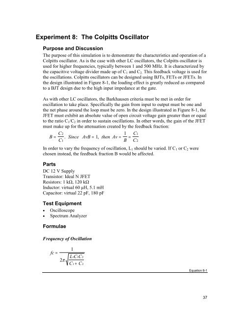
<strong>Experiment</strong> 8: The Colpitts Oscillator<br />
Purpose and Discussion<br />
The purpose of this simulation is to demonstrate the characteristics and operation of a<br />
Colpitts oscillator. As is the case with other LC oscillators, the Colpitts oscillator is<br />
used for higher frequencies, typically between 1 and 500 MHz. It is characterized by<br />
the capacitive voltage divider made up of C 1 and C 2. This feedback voltage is used for<br />
the oscillations. Colpitts oscillators can be designed using BJTs, FETs or JFETs. In<br />
the design illustrated in Figure 8-1, the loading effect is greatly reduced as compared<br />
to a BJT design due to the high input impedance at the gate.<br />
As with other LC oscillators, the Barkhausen criteria must be met in order for<br />
oscillation to take place. Specifically the gain from input to output must be one and<br />
the net phase around the loop must be zero. In the design illustrated in Figure 8-1, the<br />
JFET must exhibit an absolute value of open circuit voltage gain greater than or equal<br />
to the ratio C 1 /C 2 in order to sustain oscillations. In other words, the gain of the JFET<br />
must make up for the attenuation created by the feedback fraction:<br />
B C 2<br />
C Since AvB then Av 1 C1<br />
= . = 1,<br />
= =<br />
1<br />
B C2<br />
In order to vary the frequency of oscillation, L 1 should be varied. If C 1 or C 2 were<br />
chosen instead, the feedback fraction B would be affected.<br />
Parts<br />
DC 12 V Supply<br />
Transistor: Ideal N JFET<br />
Resistors: 1 kΩ, 120 kΩ<br />
Inductor: virtual 60 µH, 5.1 mH<br />
Capacitor: virtual 22 pF, 180 pF<br />
Test Equipment<br />
• Oscilloscope<br />
• Spectrum Analyzer<br />
Formulae<br />
Frequency of Oscillation<br />
fc =<br />
2π<br />
1<br />
LCC<br />
C + C<br />
1 1 2<br />
1 2<br />
Equation 8-1<br />
37
38 <strong>Understanding</strong> <strong>RF</strong> Circuits with Multisim<br />
Gain<br />
Av = -g m r d<br />
Equation 8-2<br />
Condition for Oscillation<br />
Av ≥<br />
C<br />
C<br />
2<br />
1<br />
Equation 8-3<br />
Procedure<br />
Figure 8-1<br />
1. Connect the circuit components illustrated in Figure 8-1.<br />
2. Double-click the oscilloscope to view its display. Set the time base to 200 ns/Div<br />
and Channel A to 10V/Div. Select Auto triggering and DC coupling.<br />
3. Select Simulate/Interactive Simulation Settings, and select Set to Zero for Initial<br />
Conditions.<br />
4. Start the simulation. When the oscillator has stabilized, measure the frequency of<br />
oscillation.
The Colpitts Oscillator 39<br />
5. Compare with theoretical calculations:<br />
f c = measured = calculated<br />
6. Stop the simulation and place a Spectrum Analyzer on the workspace.<br />
7. Connect the output lead of the oscillator to the input of the Spectrum Analyzer.<br />
8. Double-click to open the Spectrum Analyzer window.<br />
9. Press Set Span. Set Start = 10 kHz, End = 10 MHz, Amplitude = Lin and Range =<br />
2V/DIV. Press Enter.<br />
10. Restart the simulation. When the oscillation has stabilized, drag the red marker to<br />
the position of the spectrum line observed. Note the frequency in the lower left<br />
corner of the Spectrum Analyzer window:<br />
f c =<br />
11. Calculate L 1 necessary to achieve a frequency of oscillation of 8 MHz. Replace L 1<br />
by double-clicking on it and selecting Replace. Run the simulation to verify your<br />
calculation.<br />
12. Given that g m = 1.6 ms and r d = 12 kΩ, determine whether oscillations will be<br />
sustained.<br />
Expected Outcome<br />
Figure 8-2 Oscilloscope Display of Initial Colpitts Oscillator Oscillations<br />
Additional Challenge<br />
Re-design the circuit of Figure 8-1 choosing values of C 1 and C 2 so that Avβ = 10 and<br />
the frequency of oscillation is approximately 3 MHz. Replace existing simulated<br />
component values by double-clicking on the component of interest. Run the<br />
simulation and compare the output data with expected theoretical values.
40 <strong>Understanding</strong> <strong>RF</strong> Circuits with Multisim