Generating Optimal Curves via the C++ Standard Library

GENERATING OPTIMAL CURVES 

++ 

VIA THE C STANDARD LIBRARY 

ANDERS LINNÉR 

Northern Illinois University, DeKalb 

Recent computational breakthroughs in infinite-dimensional optimization have produced explicit, 

as well as numerically advantageous, gradient formulas. By following the negative gradient 

trajectories, along so-called steepest descent, the minimizing curve is sought. The C 

++ 

standard 

library supports the assembly of a user-defined type based on the standard cubic splines, and a 

corresponding operator algebra that is capable of representing all the gradient expressions while 

preserving the conventional notation. It is crucial that the algebra implements, and is ‘closed’ 

under, composition with both user-defined and built-in functions, as well as the calculus 

operations integration and differentiation. Examples illustrate both fixed and free endpoints, and 

particular attention is paid to the notoriously difficult isoperimetric constraints. In the spirit of 

‘component technology’, the implementation uses the ‘boost extension’ of the standard library and 

adapts efficient legacy code from the book ‘Numerical Recipes in C’. By limiting the choice of 

numerical methods to the most elementary algorithms, the strength of the gradient formulas is 

showcased as a general class of problems is successfully attacked using built-in generic algorithms 

with dynamic memory allocation, as well as object-oriented concepts such as inheritance. 

++ 

Categories and Subject Descriptors: G.4 [Mathematical Software]: Language Classification- C 

General Terms: Algorithms, Design, Experimentation, Performance 

Additional Key Words and Phrases: Calculus of Variations, Steepest Descent, Infinite 

Dimensional, Gradients 

1. INTRODUCTION 

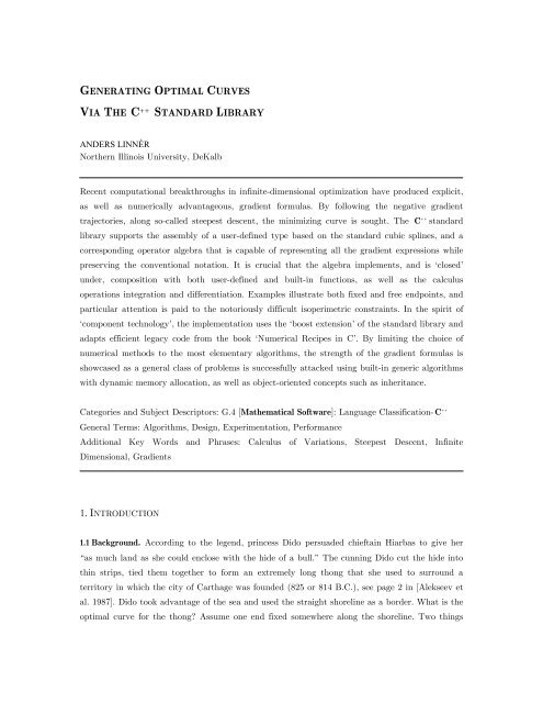
1.1 Background. According to the legend, princess Dido persuaded chieftain Hiarbas to give her 

“as much land as she could enclose with the hide of a bull.” The cunning Dido cut the hide into 

thin strips, tied them together to form an extremely long thong that she used to surround a 

territory in which the city of Carthage was founded (825 or 814 B.C.), see page 2 in [Alekseev et 

al. 1987]. Dido took advantage of the sea and used the straight shoreline as a border. What is the 

optimal curve for the thong Assume one end fixed somewhere along the shoreline. Two things

2 


must be determined, where should the final point of the thong be placed and what shape should 

the thong have between its endpoints 

1.2 Isoperimetric constraints. This legend offers one of the earliest examples of a problem where 

the optimal curve is to be determined. Dido’s problem illustrates the presence of side conditions 

since the length of the competing curves is fixed and the endpoints must be on the shoreline. 

There is of course a limitless collection of problems involving optimal curves subject to side 

conditions. The purpose of the present paper is to present an implementation that efficiently 

‘improves’ the shape of a given initial curve until the optimal curve is reached. The process is 

applicable to the general case, and all side conditions are satisfied at each stage. Any side 

condition that can be expressed as the demand that a certain integral takes on a fixed value is 

referred to as an isoperimetric constraint. Fixing the length of the competing curves is an example 

of an isoperimetric constraint. The implementation allows up to two isoperimetric constraints and 

any combination of fixed or free endpoints. The software is designed to readily extend to cases 

with more than two isoperimetric constraints, or when a point other than an endpoint is fixed, or 

if periodic boundary conditions are imposed, or any combination of the above. 

1.3 Infinite-dimensional domain with curvature. It is important to recognize that the presence of 

isoperimetric constraints introduces an essential non-linearity. The objective and the isoperimetric 

constraints typically involve integrals with integrands depending on derivatives of the function 

representing the curve. The form of the integrand suggests a choice of a linear function space of 

sufficiently smooth functions. To increase the likelihood that there is an optimal curve, the 

selected function space is the least restrictive as far as assumptions on smoothness. The subset of 

functions that satisfy an isoperimetric constraint inside the selected function space will neither be 

linear nor flat. 

1.4 Inner products. Geometric methods are made accessible once an inner product is defined on 

the function space. There is some freedom in this choice and the present paper discusses three 

different inner products. The corresponding so-called Sobolev spaces have the same properties as 

far as convergence is concerned, but they differ in subtle ways geometrically. The subset of curves 

satisfying a given isoperimetric constraint is expected to have a well-defined one-dimensional 

normal space inside the linear space of all curves. The infinite-dimensional linear space of 

functions perpendicular to this space is the so-called tangent space. Different curves typically 

correspond to different tangent spaces. The constrained curves form an infinite-dimensional ‘level 

surface’ inside the space of all curves. When two isoperimetric constraints are present, it is often 

the case that the corresponding level surfaces intersect ‘transversally’ and the normal space to the 

intersection manifold is two-dimensional. The corresponding orthogonal tangent space is of course 

still infinite-dimensional.

++ 

GENERATING OPTIMAL CURVES VIA THE C STANDARD LIBRARY 3 

1.5 Derivatives and gradients. The next step is to compute the so-called Gateaux derivative (or 

directional derivative) of the non-linear objective and constraint functionals. These derivatives are 

linear functionals and the Riesz theorem guarantees that there is a function, the gradient, which 

represents the Gateaux derivative. If the level surfaces are regular and the intersections are 

transversal, then he gradients of the constraints are in the normal space. It follows that the 

gradient of the objective can be projected onto the tangent space. There is now a curve, the 

gradient trajectory, inside the infinite-dimensional manifold with the property that its velocity 

vector is parallel to the projected gradient. The implementation presented here generates points 

along the gradient trajectory. These points correspond to ever improving curves that satisfy the 

constraints of the original problem. 

1.6 Motivation. Although the classical problems, such as Dido’s, are interesting in their own 

right, they are not the main motivation behind the development of this code. The real interest is 

in problems of periodic orbits that require ‘floating’ boundary conditions constrained to infinitedimensional 

manifolds that are not flat. In these problems the solution is not given by some 

traditional boundary-value problem such as the one related to the Euler-Lagrange equation. As 

an example consider a distorted sphere E (for Earth). A geodesic on E is a curve x such that if 

a particle travels along x with constant speed, then its acceleration vector is at all times normal 

to E . Given a tangent vector v at p in E there is a geodesic emanating from p with initial 

direction v . This geodesic extends indefinitely producing a curve that winds around E . If the 

geodesic returns to p and its direction at that instant is v , then it is said to be periodic. In the 

case of the standard round sphere each geodesic is periodic, and in fact a great circle traversed 

repeatedly. For a distorted sphere it is not clear that there are any periodic geodesics. 

1.7 Recent progress. The work of many mathematicians over several hundred years culminated in 

the 1990’s with the papers [Franks 1992; Bangert 1993; Hingston 1993]. It is now known with 

certainty that any distorted sphere has an infinite number of geometrically distinct periodic 

geodesic. Moreover, if n( L ) is the number of periodic geodesics of length less than or equal to L , 

then n( L ) grows at least as fast as the prime numbers. It is possible to generalize the notion of 

geodesics to arbitrary so-called Riemannian manifolds. In this generalized setting the Newtonian 

evolution of a mechanical system corresponds directly to a geodesic in the appropriate 

Riemannian manifold. Periodic orbits that are sought in the famous celestial three-body problem 

thus correspond to periodic geodesics. 

1.8 Current research. To the best of the author’s knowledge, nobody has successfully implemented 

an algorithm capable of generating general periodic geodesics. One difficulty is the fact that there 

is no guarantee that through a given point p with given direction v there is a periodic geodesic. 

It follows that the implementation must handle ‘floating constraints’ where p and v are allowed 

to vary keeping endpoints in agreement as in x( 0) = x( 1) 

= p and x′ ( 0) = x′ 

( 1) 

= v . This has

4 


turned out to be a considerable challenge. A second source of difficulty is the trivial fundamental 

group of the sphere. Although it is possible to find two distinct periodic geodesics in a torus by 

shrinking a pair of suitable closed curves, this approach will not work in a sphere. A third 

difficulty is the available freedom in the parameterization of the curve. Moreover, for periodic 

orbits there is also a rotation that leaves the curve invariant. The methodology of projected 

gradients combined with steepest descent adapts very well to these circumstances. Since the 

steepest descent takes place along a curved infinite-dimensional manifold, Newton’s method is not 

available as an alternative. 

1.9 Notation. Let X be a space of curves and consider functions F : X → R . The concern of this 

paper is the search for ˆx ∈ X with the property that F( xˆ 

) ≤ F( x) 

for all x ∈ X . The examples 

are drawn from the Calculus of Variations, so the space X is some subset of sufficiently smooth 

functions defined on the closed interval [ 0,1 ]. Let x = dx/ 

dt be the derivative and define 

1 

( ) ( ( ) ( )) 

F x = ∫ f t, x t , x t dt , 

3 

0 

where f : R → R is a given function. It is often assumed that the endpoints are fixed so that 

x( 0) 

= x0 

and x( 1) 

= x1 

for some specified x , x ∈ R . To expose potential candidates for ˆx 

0 1 

the conventional approach utilizes the Euler-Lagrange equation 

d ∂f ∂f 

( tx , ( t) , x( t) 

) = ( tx , ( t) , x( t) 

). 

dt ∂x 

∂x 

Here ∂f 

/ ∂ x represents the partial derivative of f with respect to its second variable, and 

∂f 

/ ∂ x the partial derivative with respect to its third variable. This ordinary differential 

equation together with the prescribed boundary conditions is an example of the classical 

boundary value problem. The basic numerical method for this typically nonlinear problem is the 

so-called ‘shooting method’ [Conte et al. 1980; Burden et al. 1985; Flowers 1995]. For a more 

comprehensive overview, including the finite element method, consult the books [Prenter 1975; 

Glowinski 1984, Nocedal et al. 1999]. The endpoint constraints cause next to no harm since the 

corresponding domain of functions is at worst a translated linear space. In contrast, suppose 

X = G −1 ( 0) 

for some functional G : H → R of the form 

1 

( ) ( ( ) ( )) 

G x = ∫ g t, x t , x t dt , 

0 

defined on some suitable Hilbert space H , and with g : R → R a given function. Typically, the 

domain X is not ‘flat’, which leads to considerable complications. In the classical theory, 

Lagrange multipliers are introduced to deal with this kind of ‘isoperimetric constraint’. 

Algorithms, such as the shooting method, are not designed to deal with unknown parameters like 

the multipliers. Line-searches are not expected to yield points in X . Alternative methods must be 

developed and the present paper explores one promising approach. 

3

++ 


1.10 Purpose and design issues. The paper presents the implementation of a general-purpose 

algorithm designed to at least handle all the standard problems in the elementary Calculus of 

Variations. The algorithm takes advantage of recent computational breakthroughs in infinite 

dimensional calculus [Linnér 2000]. There are now ‘explicit’ and ‘numerically friendly’ gradient 

formulas in terms of a certain Euler operator and the ‘Work’ functional. Flexibility in the choice 

of inner product in the Hilbert space is also permitted. Perhaps surprisingly, only very elementary 

numerical methods are sufficient as building blocks as the algorithm is assembled. The gradient 

formulas involve a mix of integrals, derivatives, compositions with special functions, and the usual 

algebraic operations. The gradient formulas are somewhat complicated and each isoperimetric 

constraint introduces its own gradient. The presence of endpoint constraints changes the gradient 

formulas and so does a change of the inner product in the function space. Given this multitude of 

different formulas, it is obviously desirable that all mathematical expressions are represented by 

code that mimics the original expressions and thus facilitating error-free translations. The pursuit 

of the infinite time limit along the negative gradient trajectories necessitates very efficient code. 

1.11 Programming language. The adoption of a C ++ standard in 1997 [Stroustrup 1997] and its 

++ 

incorporation of most parts of the Standard Template Library [Stepanov-Lee 1995] makes C a 

very attractive choice. The code is easily ported and concerns about computational speed are at 

the core of the design of the STL. Specifically, the C ++ standard library supports a flexible 

representation of the functions in the infinite-dimensional space using dynamic memory allocation. 

++ 

The C operator feature is essential to preserve standard mathematical notation. Object-oriented 

‘inheritance’ combine with the ‘boost extension’ [http://www.boost.org; Josuttis 1999] to supply 

the necessary algebra with minimal coding. It is shown how both built-in functions and userdefined 

functions can be represented as function objects capable of proper interaction with the 

discrete representation of the target functions. By demanding that all operations return an object 

of the same type, a computationally ‘closed’ framework is created. The gradient formulas are 

readily expressed in this framework, and steepest descent algorithms are easy to implement. The 

target functions are represented by cubic splines and implemented by modernizing and extending 

code in Numerical Recipes in C [Press et al. 1992]. 

1.12 Fundamental difficulty. Recall that the steepest descent is the flow along the trajectories of 

the negative gradient vector field. In all but the simplest cases this flow is not known explicitly. 

All numerical algorithms will suffer from an irreversible loss of information at the start of the 

descent in the infinite dimensional case. The initial point is a curve that can only be represented 

by a finite number of points. The flow subsequently acts on the discrete representation and this 

severely limits the number of applicable numerical tools during the descent. To deal with this 

difficulty, curves and gradients are here represented as instances of a C ++ class S (S for spline) 

with the following capabilities. S is derived from the ‘boost extension’ to give it all the usual 

algebraic operations. In addition, S has integral and derivative member functions that produce

6 


objects of class S. S has a friend FunctionObject to permit composition with library functions and userdefined 

functions. The ability to compose with functions and still have an object of class S is 

crucial when expressing the gradients. S has a Show() method that displays the values at all the 

sample points, and a Save() method to save the points and the values in a file. 

1.13 Organization. Section 2 introduces eight examples in increasing order of difficulty. The 

following table indicates if the corresponding solutions are known explicitly, implicitly or in terms 

of special functions: 

example number 1 2 3 4 5 6 7 8 

isoperimetric constraints 0 0 0 0 0 1 1 2 

number of free ends 0 0 0 0 1 0 1 2 

trivial explicit solution 

implicit/special functions 

Each example is illustrated by computer graphics. The two question marks indicate that the 

author is unaware of any rigorous derivation of these solutions in either implicit form or in terms 

of special functions. To use the implementation the user supplies a file where the types of 

constraints are indicated. For each functional the integrand and its partial derivatives must be 

coded, and an initial curve that satisfies all the constraints is coded as well. The gradient 

formulas are introduced in Section 3, and there is also a brief discussion of the influence of the 

choice of metric on the steepest descent in the space of curves. Section 3 shows how to deal with 

isoperimetric constraints. Finally, the spline class S is presented in Section 4 together with parts 

needed from the boost library along with extensions to the Numerical Recipes in C. Section 5 

gives a reference to the complete software package and also a few remarks about the testing 

under UNIX and Windows. 

Finally, I like to take this opportunity to thank the three referees and the editor for proposing a 

series of concrete improvements to the original manuscript. 

2. EXAMPLES 

2.1 Minimizing length. The first example involves the familiar length functional given by 

1 

2 

( ) = 1 + ( ) 

0 

F x ∫ x t dt . 

This simple example is useful as an introduction since the solution is known to be the straight 

line-segment connecting the two endpoints. Assume x ( 0) 

= 0 and x ( 1) 

= 2. To get a good 

6 

illustration of steepest descent, let the initial curve be given by x ( ) 

0 

t = 2t 

. The initial curve is 

coded by supplying the underlined part in: 

double initial(double t){return 2.0*std::pow(t,6);}

++ 


The convention is that reserved words in C ++ are in boldface. Names from the C ++ standard 

library or the boost extension are in italic. All other names are in regular type. This way it is 

clear at a glance which of the names must be remembered and which names are invented. The 

code corresponding to the initial curve is omitted in the subsequent examples. Next, the user 

supplies the function f and the partial derivatives ∂f / ∂ x = fx 

, ∂f / ∂ x 

= f 

. Here is the code: 

f = Sqrt(1.0 + xDot*xDot); fx = 0.0*x; fxDot = xDot/Sqrt(1.0 + xDot*xDot); 

(It is possible to modify the code so that these calculations can be performed discretely by ‘other 

programs’. If this is the case the actual data points of x and xDot must be exposed through some 

additional interface.) The names x, xDot correspond to objects of class S. The S-algebra creates S 

objects from expressions like 1.0 + xDot*xDot, and 0.0*x. Observe that 0.0 by itself is not an S-object, 

so the compiler will not accept fx = 0.0. The decision to prohibit this assignment supports type 

safety. All the standard functions are already converted to function objects as in 

FunctionObject Sqrt(std::sqrt); 

Each picture shows curves at increasing times along the descent. The negative gradient 

trajectories extend indefinitely and there is an exponential slowing as the limit is approached. To 

increase the flow-time interval between stored curves there is a user-supplied constant that can be 

used to exponentially increase the time separation between each save. To simplify the 

interpretation, curves are plotted with a lighter gray that darkens as the flow time increases. 

Only the solution is plotted in black. 

x 

2 

Example 1 

1 

Example 2 

1.75 

0.75 

1.5 

0.5 

1.25 

0.25 

1 

0.75 

-0.25 

0.5 

-0.5 

0.25 

-0.75 

-1 

2.2 Euler-Lagrange. The second example involves the functional 

1 

2 ( ) ( ) 

2 

( ) 

F x = ∫ x t + x t dt . 

0

8 


Assume that x ( 0) 

= 0 and x ( 1) 

= 1. It is tempting to believe that the solution is given by a 

straight line since making x smaller necessarily increases x and conversely. To get a nice 

illustration the steepest descent is applied to the initial curve x ( ) 

0 

t = sin( 9 πt/ 2) 

. The 

minimizing curve is not a straight line. This time the code is: 

f = x*x + xDot*xDot; fx = 2.0*x; fxDot = 2.0*xDot; 

The functional is the square of a standard norm in the Hilbert space of functions with the integral 

of the square of the derivative finite. It is possible to show that there is a function of minimal 

norm in the space of functions satisfying the boundary condition. The classical theory proves that 

the Euler-Lagrange equation must be satisfied at the minimum provided the solution is 

sufficiently differentiable. In the current example the Euler-Lagrange equation simplifies to 

x = x . The general solution is a linear combination of the hyperbolic functions sinh and cosh . 

The only solution that satisfies the boundary conditions is x( t) = sinh ( t) / sinh( 1) 

, which agrees 

with the solution generated by the implemented algorithm. 

2.3 Less smoothness. The third example illustrates a steepest descent flow towards a curve with 

discontinuous derivative. The functional is given by 

1 

2 2 

( ) = ( 1 − ( )) 

0 

F x ∫ x t dt . 

Observe that F( x) ≥ 0 , and a curve with derivative ± 1 yields equality. Assume 

x( 0) = x( 1) 

= 0, with initial curve x ( ) 

0 

t = t( t - 1/11)( t - 13/17)( t - 1) . 

The code is given by: 

f = (1.0 - xDot*xDot) * (1.0 - xDot*xDot); fx = 0.0*x; fxDot = -4.0*xDot*(1.0 - xDot*xDot); 

0.4 

0.3 

0.2 

0.1 

Example 3 

-0.05 

-0.1 

-0.15 

-0.2 

-0.25 

Example 4 

-0.1 

2.4 Brachistochrone with fixed endpoints. Consider a particle that glides without friction along a 

curve in a vertical plane. Assume that the gravitational force is the only cause of the motion. The 

curve that yields the shortest time to traverse the curve between a pair of given points is known 

as the brachistochrone with fixed endpoints. Assume the initial point is given by x ( 0) 

= 0 with 

gravity acting in the negative direction so that x( t) ≤ 0 . Assume the initial speed is given by 

v 

0 

> 0 . The functional is given by 

F x 

( ) 

= 

1 

∫ 

2 

0 

v0 

2 

( ) 

( ) 

1 + x 

t 

− x t 

dt .

++ 


It is often assumed that v 0 

= 0 , but this leads to an unbounded integrand and a number of 

related technical difficulties. The code is given by: 

f = Sqrt(1.0 + xDot*xDot)/Sqrt(v0*v0 - x); 

fx = 0.5 * Sqrt(1.0 + xDot*xDot)/( Sqrt(v0*v0 - x)*(v0*v0 - x) ); 

fxDot = xDot/( Sqrt(1.0 + xDot*xDot)*Sqrt(v0*v0 - x) ); 

The initial curve is given by x ( ) 

0 

t = 0 and the initial speed throughout is given by v 0 

= 0.2 so 

that F( x ) = 5 at the start. Observe that the integrand f does not depend on t explicitly. The 

classical approach takes advantage of this fact and the ‘second’ Euler-Lagrange equation is 

derived as f ( t, x( t) , x( t) 

) − x( t) f ( , ( ), ( )) 

x 

t x t x t = constant; [Weinstock 1974; Troutman 1983; 

Gelfand et al. 2000]. Using the second Euler-Lagrange equation it is possible to express the 

solution as a parameterized curve t = t ( τ ) and x = x ( τ ). It should be pointed out that 

neither t nor τ corresponds to time. The curve turns out to be a cycloid. It is possible to change 

the parameter to the arc-length parameter s and get explicit formulas t = t ( s) 

and x = x ( s) 

[Dombrowski 1996]. To use the parametric formulas and get the optimal ˆx ( t ) produced by the 

steepest descent algorithm, it is necessary to solve a transcendental equation. This explains why 

ˆx ( t ) is never given explicitly in the literature. The graph of the function ˆx ( t ) produced by the 

algorithm and the trace of the parametric curve ( t ( τ) , x ( τ )) 

are the same. 

2.5 Brachistochrone with a free endpoint. If it is only required that the curve reaches the vertical 

line t = 1 , then the right-hand endpoint is said to be free. Since the Euler-Lagrange equation is a 

second order equation, its solutions have two constants that must be determined. In the case of a 

free endpoint a second necessary condition is therefore required. The condition, known as a 

‘natural’ boundary condition [Gelfand et al. 2000; Troutman 1983], is in general given by 

f ( 1, ( 1 ), ( 1 )) 

x x x = 0 . In the case of the brachistochrone this simplifies to x ( 1) 

= 0. In the 

implementation there is no need to change any of the code assuming. All that is needed is the 

information that the right-hand endpoint is free. This will activate a different set of gradient 

formulas behind the scenes. In general it is possible to have the left-hand endpoint free or both 

endpoints free. In any case the corresponding gradient formulas are known and there is no need to 

change any of the code. 

Example 6 

-0.2 

Example 5 

-0.4 

-0.1 

-0.2 

-0.3 

-0.4 

-0.5 

-0.6 

-0.6 

-0.8 

-1

10 


2.6 Length constrained brachistochrone with fixed endpoints. Since it is possible to give a 

parametric representation in terms of the arc-length parameter, it follows that the length L 0 

of 

the brachistochrone is known. Consider now the following problem. Choose a length L 1 

different 

from L 

0 

and determine the curve ˆx of length L 1 

with F( xˆ 

) ≤ F( x) 

for all curves of length L 1 

satisfying the boundary conditions. This is an example of an isoperimetric problem. In addition to 

1 

2 

1 + x 

( t) 

F( x) 

= ∫ 

dt , 

2 

( ) 

0 

v0 

− x t 

there is also the constraint functional 

1 

2 

( ) = 1 + ( ) 

0 

G x ∫ x t dt . 

Assume that x ( 0) 

= 0, and let the initial curve be given by ( ) 2 

x t = − t t so that 

0 3 

( ) 2 

x 1 = − . The appropriate gradient formulas keep both the endpoints fixed. This particular 

3 

initial curve is useful since its length is known to be exactly equal to 14 / 9 . With f as before the 

additional code is given by: 

g1 = Sqrt(1.0 + xDot*xDot); g1x = 0.0*x; g1xDot = xDot/Sqrt(1.0 + xDot*xDot); 

2.7 Length constrained brachistochrone with a free endpoint. Unlike the case with both endpoints 

fixed, it is possible to use a straight segment as the initial curve. Let x ( ) 

0 

t = − t so that the fixed 

length is given by 2 . This time the ‘natural’ boundary condition involves a Lagrange multiplier 

associated with the isoperimetric constraint. It is therefore in general not possible to draw 

conclusions about the geometry of the optimal curve at the free endpoint. In contrast, the two 

concerns about the endpoint and the fixed length are kept separate in the implementation. One is 

resolved by the choice of gradient formula, and the other is handled by the projection onto the 

proper tangent space. 

Example 8 

Example 7 

-0.2 

-0.4 

-0.6 

-0.8 

-1 

2.8 Multiple isoperimetric constraints. Another one of the oldest examples in the calculus of 

variations is the elastic curve. The problem is to minimize the elastic energy of a wire with fixed

++ 


endpoints. Since the optimal curve need not be a graph of a function it is reasonable to let the 

tangent angle represent the curve. It is also convenient to choose a parameter proportional to the 

arc-length since this circumvents the fixed length constraint. Let x( t ) correspond to the tangent 

∫ 

t 

angle and plot t ( cos ( x( s) 

), sin ( x( s) 

)) 

ds . The elastic energy is proportional to 

0 

1 

2 

( ) ( ) 

0 

F x = ∫ x t dt . 

To keep the endpoints fixed the following constraints hold 

1 

( ) ( ( )) 

1 

cos 

0 

G x = ∫ x t dt , G ( x) = sin( x( t) 

) 

∫ dt . 

2 

The initial tangent curve is given by x ( ) 

0 

t = 3 πt 

− π/2. The corresponding curve is a circle and 

a half. By letting the ends rotate freely, it is possible to reduce the elastic energy dramatically. 

g1 = Cos(x); g1x = (-1.0)*Sin(x); g1xDot = 0.0*x; 

g2 = Sin(x); g2x = Cos(x); g2xDot = 0.0*x; 

This solution shows the stable configuration of a springy wire held so that the endpoints are fixed 

but with free tangent directions. There is no bending at the endpoints and hence the second 

derivative is zero. If, unlike here, the symmetry of reflection is preserved during steepest descent, 

then the limit curve will not be the minimal energy configuration. 

1 

0 

2.9 Convergence criterion and computational speed. In all the examples the limit curve drawn in 

black corresponds to a curve where the norm of the projected gradient vector field is less than 

6 

10 − . The user supplies this value along with other parameters that control the behavior of the 

algorithm. The number n of cubic splines carried by each S-object is one such important 

parameter. To measure the speed of the algorithm a method for timing generic algorithms is 

employed, see Chapter 19 in [Musser et al. 2001]. 

n b0 t0 f0 b1 t1 f1 b2 t2 f2 

4 0.46 0.27 1.30 0.99 0.53 1.60 

8 0.56 0.36 1.33 1.70 1.33 1.34 0.65 2.14 1.34 

16 1.20 0.76 2.13 3.31 2.71 2.04 1.36 4.60 2.14 

32 1.66 1.15 1.50 4.88 4.13 1.52 1.84 6.93 1.51 

64 2.78 2.01 1.75 8.47 7.40 1.79 3.08 12.3 1.76 

128 4. 81 3.60 1.79 14.9 13.6 1.84 5.21 22.6 1.83 

256 8.85 7.02 1.95 28.6 27.0 1.98 9.52 43.1 1.91 

512 16.9 13.4 1.90 55.6 55.6 2.06 18.2 81.8 1.90 

1024 33.3 29.2 2.18 111 88.9 1.60 37.0 163 1.99 

2048 66.7 58.3 2.00 250 250 2.81 71.4 429 2.63 

4096 143 107 1.84 500 500 2.00 143 857 2.00 

The results are split as baseline time b i 

(preparation of data) and computational time t i 

. The 

values are given in milliseconds and the index i corresponds to the number of isoperimetric

12 


constraints. The timing is for a Sun Ultra 5 running Solaris 7 using GNU g++ version 2.95 

compiled with speed optimization. The ratio f ( ) ( )/ ( n 

i 

n = ti n ti 

2 ) is listed and Examples 1, 6, 

and 8 are tabulated as index 0, 1, and 2 respectively. The next table lists, by example, the step 

sizes h and the number of steps taken before the norm of the projected gradient vector is zero 

6 

within the acceptable tolerance of 10 − . All constraints are satisfied to at least three significant 

digits. 

example 1 2 3 4 5 6 7 8 

n 32 64 256 128 128 512 512 128 

h 0.5 0.1 0.001 0.001 0.001 0.01 0.01 0.01 

steps 256 64 16384 20480 40960 4096 8192 512 

By combining the information in the two tables one estimates example 6 to take between 

4096 ⋅ t ( ) 

1 

512 and 4096 ⋅ ( b ( ) ( 1 

512 + t1 

512 ) milliseconds. With b ( ) ( ) 

1 

512 = t1 

512 = 55.6 

milliseconds the estimate is 4 to 8 minutes. A stopwatch trial yielded 5 minutes and 40 seconds. It 

4 

is increasingly difficult to visually distinguish between curves of tolerances less than 10 − , so in 

practice these times can often be reduced by a factor of four without a loss of geometric insight. 

3. GRADIENTS 

n 

3.1 Definitions. Given a smooth (sufficiently differentiable) function f : R → R, the directional 

n 

derivatives Df ( x ) : R → R are linear maps represented by the matrices 

⎡ ∂f 

∂f 

⎤ 

Df ( x ) = ( x ) ( x ) 

x 

⎢ 

1 

x 

. 

⎣ ∂ 

∂ n ⎥ ⎦ 

n n 

The gradient vector field ∇f 

: R → R is given by 

⎡ ∂f 

⎤ 

( x ) 

∂x 

1 

∇ f ( x) 

= . 

∂f 

( x 

) 

∂x 

⎢⎣ 

n ⎥⎦ 

Let , represent the standard Euclidean dot product. Given any 

n 

v ∈ R the formula for matrix 

multiplication shows that Df ( x ) v = ∇ f ( x ), v . This generalizes to the case F : H → R , where 

H is a Hilbert space of curves. Define the directional derivative DF : H → R by 

F( x + tv) − F( x) 

DF ( x ) v = lim 

. 

t →0 

t 

If H is equipped with the inner product , , then the gradient ∇ F is defined by the relationship 

DF ( x ) v = ∇ F ( x ), v . The existence and uniqueness of ∇ F is the content of the Riesz-Fréchet 

Theorem [Luenberger 1969]. It is important to recognize that different choices of metrics yield 

different gradient vector fields.

++ 


3.2 Projected gradients. The presence of constraints invariably leads to spaces of curves that are 

not linear subspaces. For instance, consider the space of curves with fixed endpoints. Specifically, 

let H be a Hilbert space of functions defined on [ 0,1 ] and let 

X = { x ∈ H x( 0 ) = x ( ) 

0, x 1 = x1 

}. 

X is not a linear subspace except when x 0 

= x 1 

= 0 . Let H { ( ) ( ) 

0 

= x ∈ H x 0 = x 1 = 0} 

and 

observe that X = H0 

+ x where x ( t ) = x ( ) 

0 

+ t x1 

− x0 

. X is an example of a translated 

linear subspace. Suppose F : H → R is smooth and let , be the inner product. The restriction 

of F to X has a projected gradient 

π 

π 

∇ F that satisfies ∇F 

−∇ F, v = 0 for all v ∈ H0 

. The 

gradient vector field is the tangential part of the ambient gradient vector field. In the case of 

isoperimetric constraints, things are more complicated since the tangent space is no longer a 

single fixed subspace. In either case there is a projected gradient vector field on the tangent 

bundle of X , i.e., the union of tangent spaces to X . The steepest descent takes place along the 

trajectory in X such that its velocity is always the negative of the projected gradient. 

3.3 From gradient formula to code. Let the inner product be given by 

wv , = w(0) v(0) +∫ wtvtdt ( ) ( ) . 

Suppose the functional is given by 

1 

Fx ( ) f( tx , ( t) , x( t) 

) dt 

= ∫ . 

Define the Euler operator by 

0 

1 

0 

t 

f ∂f 

∂f 

( ) ( , ( ), ( )) ( , ( ), 

( ) 

x = − 

) 

∂x 

∫ 

 

 

∂x 

0 

E t t x t x t s x s x s ds . 

In the case of fixed endpoints, the gradient formula is given by [Linnér 2000] 

t 

1 

∫ 

f 

x ∫ 

f 

x . 

0 0 

∇ Fx () = E () sds− 

t E () sds 

The gradient clearly vanishes at both endpoints. Observe that the gradient is a function that can 

be expressed in terms of x and x using operations provided by the class S. Assume that x is an 

S-object representing the current curve. The code corresponding to the gradient formula is given 

by: 

S Euler; 

Euler = fxDot – Integral(fx); 

Gradient = Integral(Euler) – Identity*CompleteIntegral(Euler); 

(Ultimately the definitions of the spline class will be placed in its own namespace (Spline say) to 

protect against name clashes, so S will be replaced by Spline::S, much the same way names from the 

standard library are prefixed by std::). The values of f, and the partial derivatives fx and fxDot are 

supplied by the user. The coded gradient formula exposes the central idea of the implementation: 

Everything representing a point in the infinite-dimensional space must be an S-object. The S-object

14 


Identity has the property that Identity(t) = t for all t. It is incorrect to replace Identity by a double t 

since this creates a gradient where the t in front of the second integral is the current value of t as 

the statement is executed. 

3.4 Different gradients due to side conditions and choice of inner product. The implementation 

supports gradient formulas for free endpoints, free left-hand endpoint, free right-hand endpoint, 

and fixed endpoints. The inner product induces a metric in the space of curves. A change in the 

metric alters the gradients. The steepest descent trajectory is different. Geometric properties, such 

as symmetries, are preserved in some metrics but not in others. Observe that, although the 

gradient depends on the metric, the collection of curves where the gradient vanishes is fixed. 

There are also differences in the level of smoothness in the gradient formulas as the metric 

changes. All gradient formulas are expressed in terms of the Euler operator and the Work integral 

1 

f ∂f 

Wx 

= ( t, x( t) , x( t) 

) dt 

∂ x 

0 

∫ . 

3.5 Examples with fixed endpoints. The most common type of constraints is to fix one or both of 

the endpoints. Computationally these constraints are easier to deal with than the unconstrained 

case. This is due to the fact that the explicitly known gradient formulas are simpler in this case. 

For instance, if both endpoints are fixed, then the corresponding gradients are given by 

π 

I 

t 

1 

f 

x 

0 0 

∫ ∫ 

∇ Fx ( ) = E ( sds ) − t E ( sds ) 

π 

II 

f 

x 

t 

1 

f 

sinh( t) 

f 

x 

x 

sinh(1) 

0 0 

t 

1 

⎧⎪ 

⎪ f 

t 

f 

x 

x 

∫ ( 1+ p)( 2− p) 

−1∫ 

⎪ 0 0 

t 

1 

f ( 1 p)( 1 t p) 

1 

⎪ ∫ x 

( 1+ p)( 2 − p) 

−1 

∫ 

0 0 

∫ ∫ 

∇ Fx ( ) = E ()cosh( s t−sds ) − E ()cosh( s b−sdt 

) 

π 

⎪ E () s ds − E () s ds 0≤ t ≤ p 

∇ 

III 

Fx ( ) = ⎨ . 

⎪⎪ 

⎪ + + − − f 

E () s ds − Ex 

() s ds p ≤ t ≤ 1 

⎪⎩ 

Here the subscript refers to the metric. The superscript indicates that this is the projected 

gradient. The three metrics are given by 

and 

wv , = w(0) v(0) +∫ wtvtdt ( ) ( ) , 

I 

1 

0 

1 1 

wv , = wtvtdt ()() + wtvtdt ()() 

II 

∫ ∫ , 

0 0 

wv , = wpvp ( ) ( ) +∫ wtvtdt ( ) ( ) . 

III 

1 

0 

The gradients are given in a form where it is obvious that they vanish at the endpoints. Another

++ 


noteworthy property is the absence of the work integral. The third metric is included here to 

illustrate how, when 0 the gradient is less smooth than when using either of the first 

two metrics. 

3.6 Examples with free right-hand endpoint. To see examples where the work integral is present, 

consider the case of a free right-hand endpoint so the projection has changed. The first two 

metrics yield 

t 

π,0 

f 

f 

∇ 

I 

Fx ( ) = ∫ Ex( sds ) + Wx 

t, 

0 

and 

t 

⎛ 1 

⎞ 

π,0 

f f f 

sinh( t) 

∇ 

II 

Fx ( ) = ∫ Ex( s)cosh( t− sds ) + Wx Ex( s)sinh( b sds ) 

− − ⎜ ∫ ⎟ cosh(1) 

0 

⎜⎝ 

. 

0 

⎠ 

It is clear that the gradients vanish at the left-hand endpoint, but not necessarily at the righthand 

endpoint. Here a second superscript indicates that only the right-hand endpoint is fixed. 

3.7 Isoperimetric Constraints. Recall that the case of fixed endpoints generated translated linear 

subspaces and the need for an orthogonal projection to compute the gradient vector field. The 

tangent space to a translated linear subspace is the linear subspace itself. Isoperimetric 

constraints G : H → R defined in a Hilbert space H are more complicated since they generate 

tangent spaces that vary from point to point. Since G( x ) = 0 for each x that satisfies the 

isoperimetric constraint G , it must be that the directional derivative satisfies DG ( x ) v = 0 for 

all tangential v , and the familiar ∇ G( x), v = 0 holds. Now consider F : H → R and its 

gradient vector field. The idea is to introduce a scalar field λ ( x ) and express the tangential 

component 

π 

π 

∇ F as ∇ F( x) = ∇F( x) −λ 

( x) ∇ G( x) 

. The condition DG ( x ) v = 0 leads to 

DG ( x ) ∇F ( x ) 

λ ( x ) = 

. 

DG ( x ) ∇G ( x ) 

For this approach to work it is necessary to assume that ∇G( x) ≠ 0 for all x such that 

G( x) 

= c. This assumption is referred to as regularity. 

3.8 Multiple isoperimetric constraints. Suppose a finite number of isoperimetric constraints 

Gi 

: H → R are invoked. Each x of interest satisfies G ( ) 

i 

x = 0 for i ∈ { 1, …, 

n} 

. This time the 

projected gradient is given by 

n 

( ) ( ) λ ( ) ( ) 

i i 

i= 

1 

π 

∇ F x = ∇ F x −∑ x ∇ G x , 

where each λ i 

is a scalar field. The additional difficulty when n > 1 is the necessity to solve the 

linear system 

⎡DG ( ) ( ) ( ) 

( ) 

1∇G1 x DG1∇Gn 

x ⎤⎡λ1 x ⎤ ⎡DG1∇F x ⎤ 

⎥⎢ ⎥⎢ ⎥⎢ = 

 

. 

⎥⎢ DG ( ) ( ) ( ) 

( ) 

n∇G1 

x DGn∇Gn x ⎥⎢λn x DGn∇F x 

⎢ 

⎣ ⎥⎢ ⎦⎣ ⎥⎦ ⎢⎣ ⎥⎦

16 


For this system to have a unique solution it is not enough for each constraint to be regular. It 

must be assumed that the matrix is invertible at each x such that G ( ) 

i 

x = 0 for all 

i ∈ { 1, …, 

n} 

. Geometrically this corresponds to transversal intersections and the dimension of 

the space normal to the tangent space is at each point equal to n . 

4. IMPLEMENTATION 

4.1 The spline class. In this section the code is dissected and the different techniques used in the 

implementation are highlighted. Objects of the class S represent the curves and the gradients. S is 

given by the following C ++ code. Reserved words are in bold. Names from either the standard 

library or the boost extension are in italic. 

#include "operators.hpp"//boost extension 

#include 

#include 

#include 

class FunctionObject;//Forward declaration 

class S : private 

boost::addable, boost::addable, 

boost::subtractable, boost::subtractable, 

boost::multipliable, boost::multipliable, 

boost::dividable, boost::dividable 

{public: friend FunctionObject; 

S(std::vector, std::vector); 

double operator()(double); 

void Show() const; void Save(const std::string&) const; 

S& operator+=(const S&); S& operator+=(const double&); 

S& operator-=(const S&); S& operator-=(const double&); 

S& operator*=(const S&); S& operator*=(const double&); 

S& operator/=(const S&); S& operator/=(const double&); 

S Integral(double) const; S Derivative() const; 

private: std::vector m_p, m_v, m_vdotdot;}; 

class FunctionObject : public std::unary_function 

{public: FunctionObject(double (*)(double)); 

double operator()(double) const; 

S operator()(const S&) const; 

private: double (*m_f)(double);}; 

A reader unfamiliar with C ++ may think of a S as an example of a user-defined type like the 

built-in double. Unlike built-in types, a user-defined type must supply functions to control creation 

and manipulation of its objects. The boost extension to the standard library will leverage these 

functions and restore some of the functionality available to built-in types. Here the extension uses 

the eight user-supplied member operators to define almost all the standard algebraic operations. 

As an example look at the boost extension’s addable class which permits the compiler to properly 

interpret the plus in expressions like x*x + xDot*xDot:

++ 


template 

class addable 

{ friend T operator+(T x, const T& y) {return x += y;} }; 

The class S has three private data members stored as dynamically allocated vectors based on the 

built-in type double. To create an object of class S representing a function x , it suffices to supply a 

discrete set of parameters p and the corresponding values ( ) 

i 

vi 

= x pi 

. The second derivative of 

the cubic spline, passing through the points ( p , v ) in order, is automatically computed and 

saved in the third data member. To illustrate this consider how the Identity object is created and 

the initial x. 

i 

i 

//Sample points 

double* p; 

p = new double[NumberOfCubicPolynomials + 1]; 

//Uniform sample 

for(unsigned int i = 0; i

18 


integral with a supplied initial value to facilitate piecewise integration. To retain notational 

compatibility with the code in the recipes, this part of the code uses indices and array notation. 

double SplineDerivativeValue(std::vector& x, std::vector& y, 

std::vector& yDotDot, double t) 

{int klo=0, khi = x.size() - 1,k; 

while( khi-klo > 1 ) 

{k=(khi+klo) >> 1; 

if(x[k] > t) khi=k; else klo=k;} 

double h,a,b; 

h = x[khi]-x[klo]; 

a = (x[khi]-t)/h; 

b = (t-x[klo])/h; 

return (y[khi]-y[klo])/h + ((1.0 - 3.0*a*a)*yDotDot[klo] + (3.0*b*b - 1.0)*yDotDot[khi])*h/6.0;} 

double SplineIntegralValue(std::vector& x, std::vector& y, 

std::vector& yDotDot, double t) 

{int klo=0, khi = x.size() - 1, k; 

while( khi-klo > 1 ) 

{k=(khi+klo) >> 1; 

if(x[k] >= t) khi=k; else klo=k;} 

double h,a,b; 

h = x[khi]-x[klo]; 

a = (x[khi]-t)/h; 

b = (t-x[klo])/h; 

return (b*b*y[khi] + (1.0 - a*a)*y[klo])*h/2.0 + 

((2.0*a*a - a*a*a*a - 1.0)*yDotDot[klo] + (b*b*b*b - 2.0*b*b)*yDotDot[khi])*h*h*h/24.0;} 

The Spline routine in the recipes updates the second derivative vector. The derivative and integral 

S member functions are given by the following code. 

S S::Derivative() const 

{S New(*this), Old(*this); 

std::vector::const_iterator pIterator = Old.m_p.begin(); 

std::vector::iterator vIterator = New.m_v.begin(); 

while( pIterator != Old.m_p.end() ) 

*vIterator++ = SplineDerivativeValue(Old.m_p,Old.m_v,Old.m_vdotdot,*pIterator++); 

Spline(New.m_p,New.m_v,New.m_vdotdot); 

return New;} 

S S::Integral(double InitialValue) const 

{S New(*this), Old(*this); 

std::vector::const_iterator pIterator = Old.m_p.begin(); 

std::vector::iterator vIterator = New.m_v.begin(); 

*vIterator++ = InitialValue; 

++pIterator; 

while( pIterator != Old.m_p.end() ) 

*vIterator++ = SplineIntegralValue(Old.m_p,Old.m_v,Old.m_vdotdot,*pIterator++); 

std::partial_sum(New.m_v.begin(),New.m_v.end(),New.m_v.begin());

++ 


Spline(New.m_p,New.m_v,New.m_vdotdot); 

return New;} 

Note how the standard library’s generic algorithm std::partial_sum in is very helpful here. 

It is interesting to compare the index-free coding style of the last two functions and the prestandard-template-library 

style of the Recipes code. The C 

++ 

standards committee exhibited 

considerable leadership when it decided to incorporate most of the standard template library 

[Stepanov et al. 1995] into the standard library. To further conform to standard mathematical 

notation it is useful to define four global functions. 

S operator-(const double& x, const S& y) {return (-1.0)*(y-x);} 

S Integral(const S& x){return x.Integral(0.0);} 

double CompleteIntegral(const S& x){return x.Integral(0.0)(1.0);} 

S Derivative(const S& x){return x.Derivative();} 

In what follows the cubic splines are shielded from the rest of the implementation, and any 

collection that provides the same functionality could take the place of the cubic splines. 

4.3 FunctionObject. The implementation of composition in the FunctionObject class is given by 

the following code. 

double FunctionObject::operator()(double t) const {return m_f(t);} 

S FunctionObject::operator()(const S& x) const 

{S result(x); 

std::transform(x.m_v.begin(),x.m_v.end(),result.m_v.begin(),*this); 

Spline(result.m_p, result.m_v, result.m_vdotdot); 

return result;} 

A FunctionObject is equipped with one ‘evaluation operator’ and one ‘composition operator’. The 

composition operator uses the evaluation operator through self-reference inside the generic 

algorithm std::transform. The abstraction built-in to the standard template library is here paying 

great dividend. 

4.4 Steepest descent. The most basic way of implementing steepest descent is with the help of 

Euler’s method. The curve is represented by an object x of class S and the gradient at x by the S- 

object Gradient. The initial curve is represented by the S-object x0. The step size is given by a 

double h. 

S x = x0, xDot, Gradient; 

xDot = Derivative(x);//Start of the Euler step 

ProjectedGradient = … 

x -= h*ProjectedGradient;//End of the Euler step 

The value of the functional is lower at this new x compared to x0. To lower the value further, 

repeat the Euler step.

20 


5. CONCLUSIONS. 

About a decade ago, while working on implementations of infinite-dimensional problems, it 

became clear to the author that it is necessary to bridge the notational gap between the 

mathematical formulas and the corresponding computer code. Back then, the coding of 

sophisticated mathematical formulas and the demand for performance yielded very frail and 

difficult to extend programs. The emergence of C ++ 

and the standard template library has 

changed all of this. As this article demonstrates, it is now possible to write code where the 

notational gap between the mathematical formulas and the computer code has all but 

disappeared. Significantly, this does not come with severe, or even noticeable, performance 

degradation. Moreover, the code here is easily extended to cover more than two isoperimetric 

constraints, or more than one metric. It is also designed to be user-friendly in the sense that next 

to no knowledge of C ++ 

is required to add code for new examples. All that is needed is a 

straightforward translation of the mathematical expressions corresponding to the integrand of 

each functional involved and its partial derivatives. The complete software package is available 

for download at: 

http://www.math.niu.edu/~alinner/Software/CoV00/ 

Testing has been done in UNIX Solaris 7 and Windows 98 Second edition using GNU g++ 

version 2.95 and Borland C++ Builder 4.0, respectively. One reasonable approach to improve the 

performance of the software is to combine the Euler step with Adams-Bashforth’s method and 

invoke higher order formulas as soon as enough points are calculated. As seen in Section 2.9, the 

subsequent freedom to aggressively increase the step size is desirable. In the context of ‘critical 

curves at infinity’ this feature is essential. Examples of this, using a completely different 

implementation, are given in [Linnér 2001]. The current implementation avoids all but the most 

basic numerical methods to showcase the strengths of the underlying gradient formulas as well as 

++ 

the power of C and the standard library. 

REFERENCES 

Alekseev, V. M., Tikhomirov, V. M., and Fomin, S. V., Optimal Control. Consultants Bureau, 

1987, 2-5 

Bangert, V., On the existence of closed geodesics on the two-sphere. Internat. J. Math. 4 no. 1, 

1993, 1-10 

Burden, R., Faires, J. D., Numerical Analysis Third edition, Prindle Weber and Schmidt 1985, 

526-532 

Conte, S. D., de Boor, C. Elementary Numerical Analysis An Algorithmic Approach, Third 

Edition, McGraw-Hill 1980, 412-416

++ 


Dombrowski, P., The Brachistochrone Problem: A Problem of Elementary Differential Geometry, 

Geometry and topology of submanifolds, VIII, World Sci. 1996, 148-167 

Flowers, B. H., An Introduction to Numerical Methods in C++, Oxford University Press 1995, 

410-413 

2 

Franks, J., Geodesics on S and periodic points of annulus homeomorphisms. Invent. Math. 108 

no. 2 1992, 403-418 

Gelfand, I. M., Fomin, S. V., Calculus of Variations. Dover 2000 

Glowinski, R., Numerical Methods for Nonlinear Variational Problems. Springer-Verlag 1984 

Hingston, N., On the growth of the number of closed geodesics on the two-sphere. Internat. Math. 

Res. Notices no. 9, 1993, 253-262 

Josuttis, N. M., The C++ Standard Library A Tutorial and Handbook, Addison-Wesley 1999 

Linnér, A., Symmetrized Curve-Straightening, To appear., Differential Geometry and its 

Applications, Preprint 2001, http://www.math.niu.edu/~alinner/ 

Linnér, A., Gradients, preferred metrics and asymmetries, Preprint 2000 

http://www.math.niu.edu/~alinner/ 

Luenberger, D. G., Optimization by Vector Space Methods, John Wiley and Sons 1969, 109 

Musser, D. R., Derge, G. J., Saini, A., STL Tutorial and Reference Guide, Second Edition, C++ 

Programming with the Standard Template Library, Addison-Wesley 2001, 279-289 

Nocedal, J., Wright, S. J., Numerical Optimization, Springer-Verlag 1999 

Prenter, P. M., Splines and Variational Methods. John Wiley & Sons 1975 

Press, W. H., Teukolsky, S. A., Vetterling, W. T., Flannery, B. P., Numerical Recipes in C, The 

Art of Scientific Computing, Second Edition, Cambridge University Press 1992, 113-116 

Stepanov, A. A., Lee, M., The standard template library. Technical Report HP-94-34, Hewlett- 

Packard, April 1994. Revised July 7, 1995 

Stroustrup, B., The C++ Programming Language Third Edition, Addison-Wesley 1997 

Troutman, J. L., Variational Calculus with Elementary Convexity, Springer 1983, 147-155 

Weinstock, R., Calculus of Variations with applications to physics and engineering. Dover 1974, 

28-29

Generating Optimal Curves via the C++ Standard Library

Create successful ePaper yourself

Delete template?

Save as template?